GT ICR - Ian Hothi - Exploring the Epoch of Reionization with Scattering Transforms

Transcript

1. Exploring the Epoch of Reionization with Scattering Transforms Ian Hothi Collaborators: Erwan Allys (LPENS) , Benoit Semelin (LUX), Romain Meriot (Imperial College), Francois Boulanger (LPENS) 1
2. The Epoch of Reionization 2
3. The Epoch of Reionization The Process Redshift, z 3
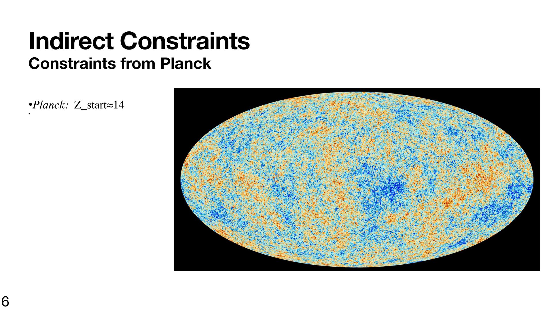
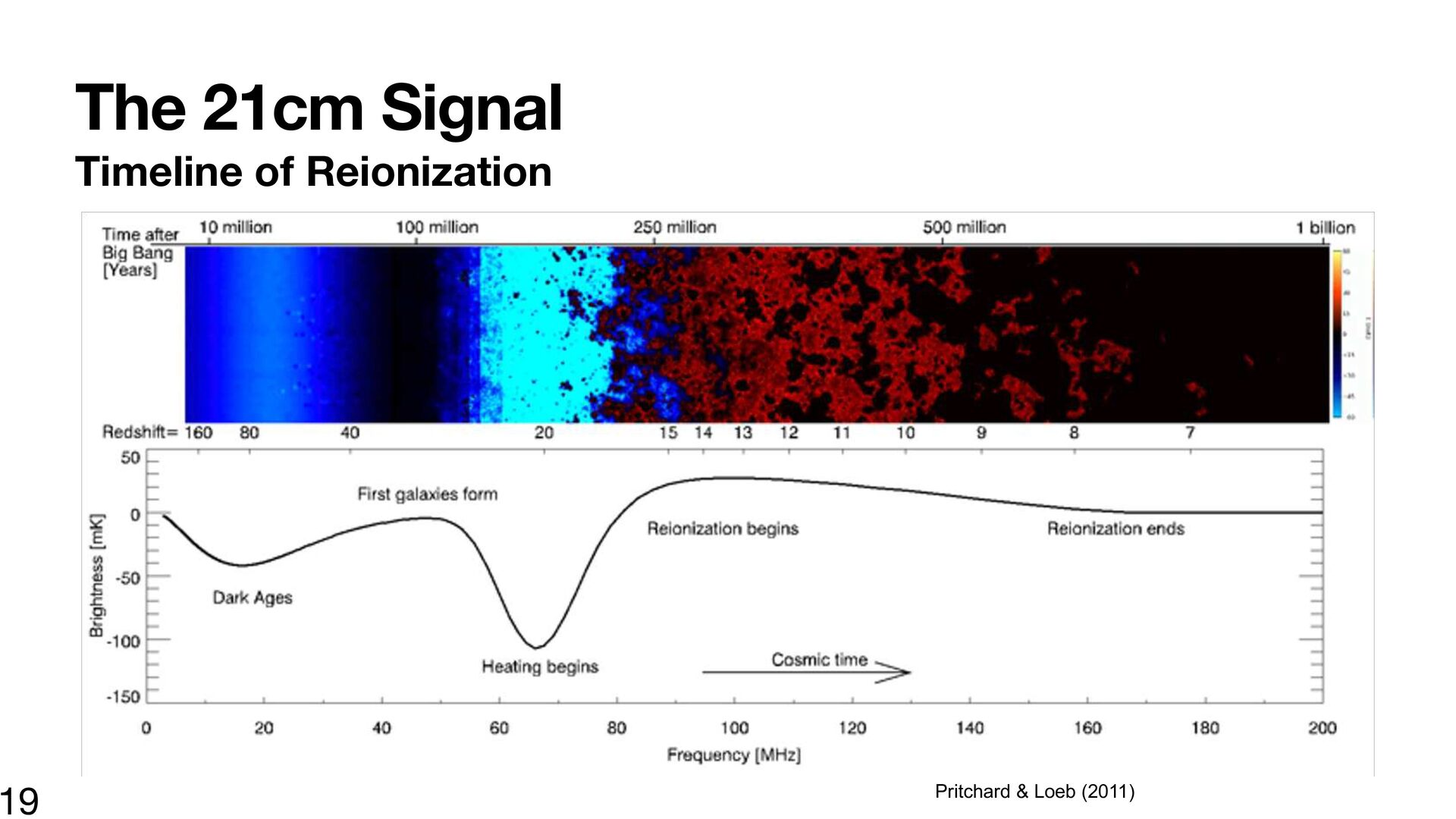
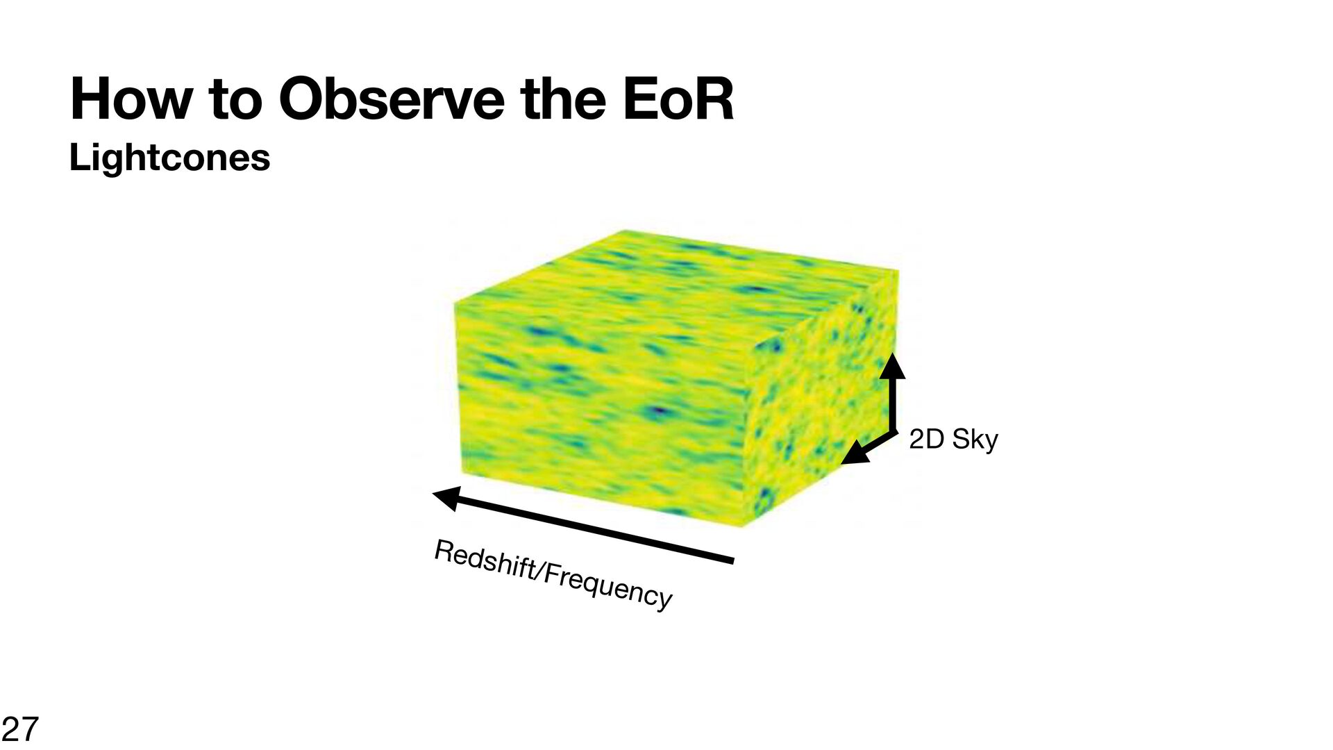
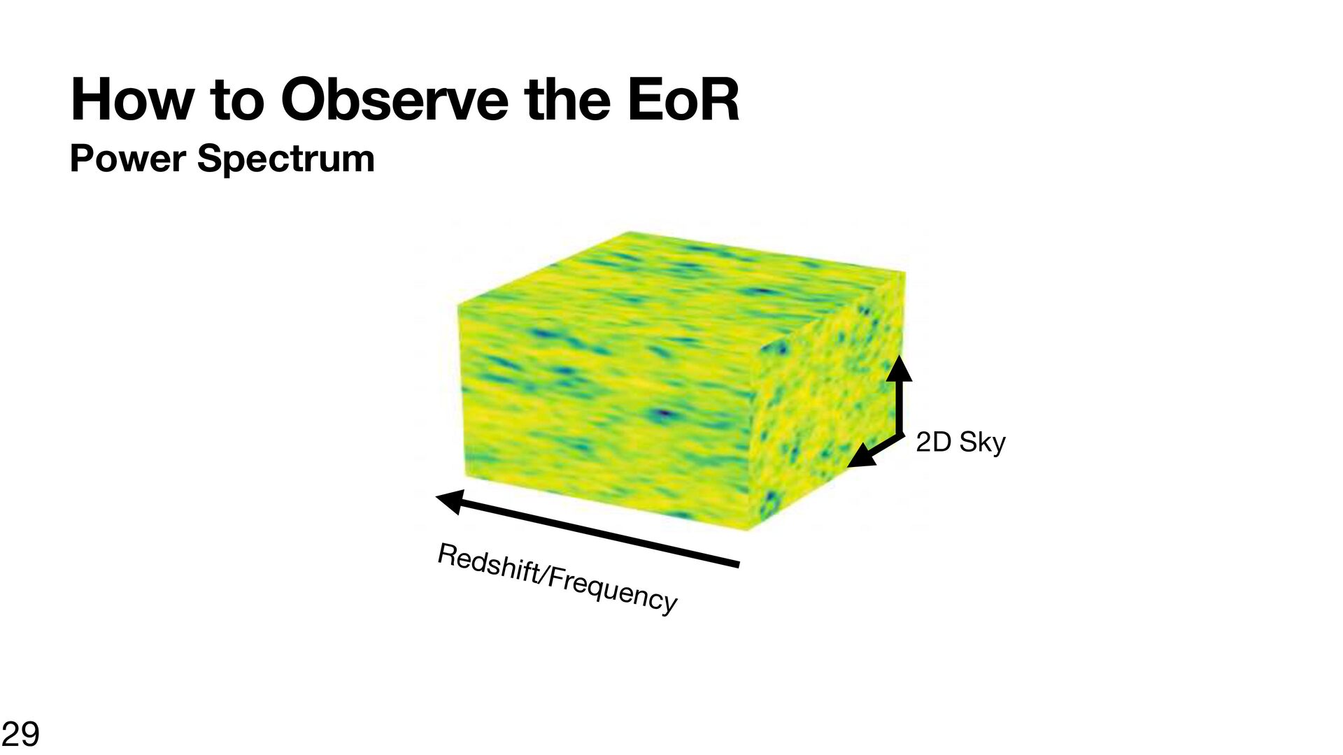
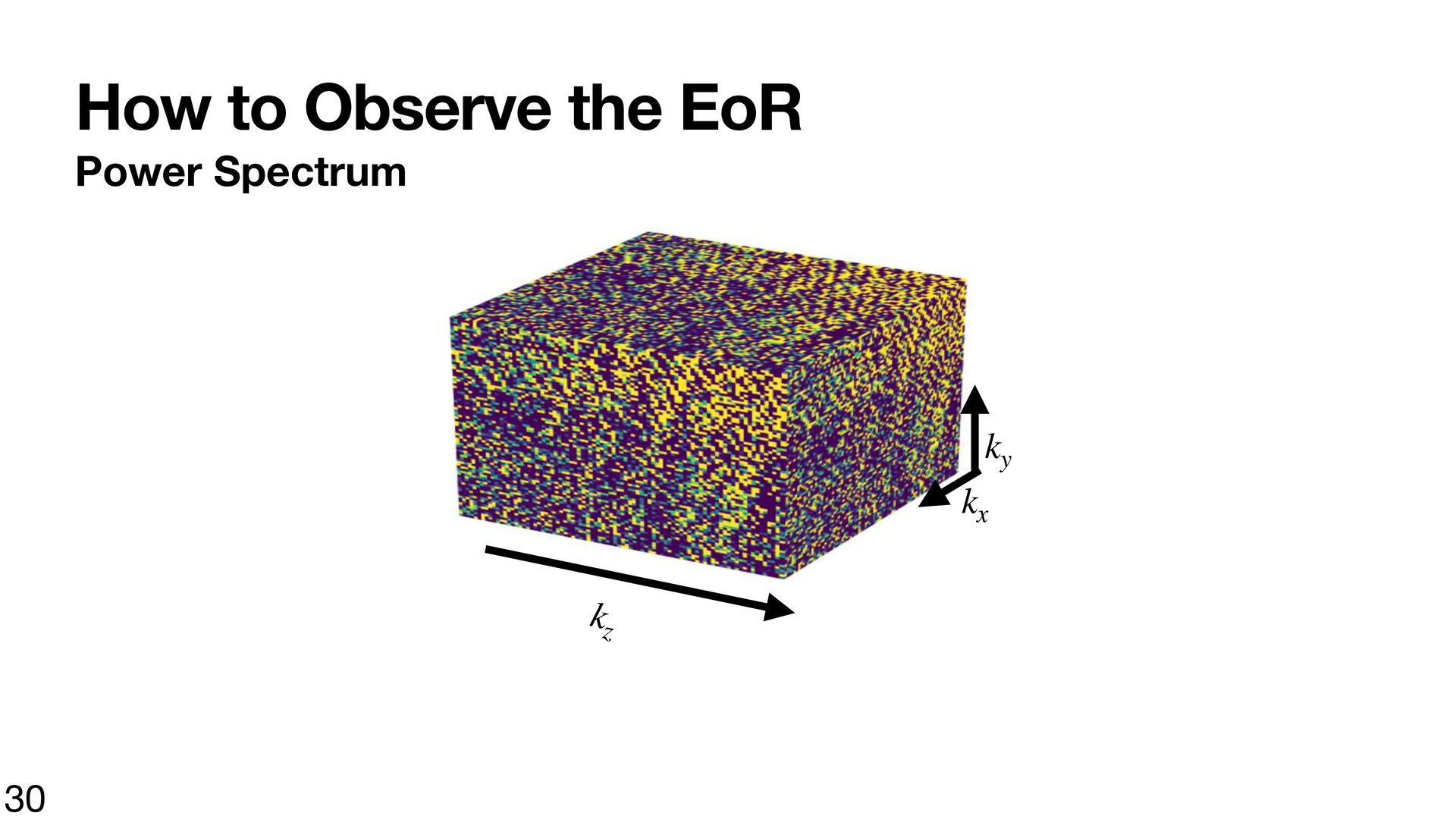
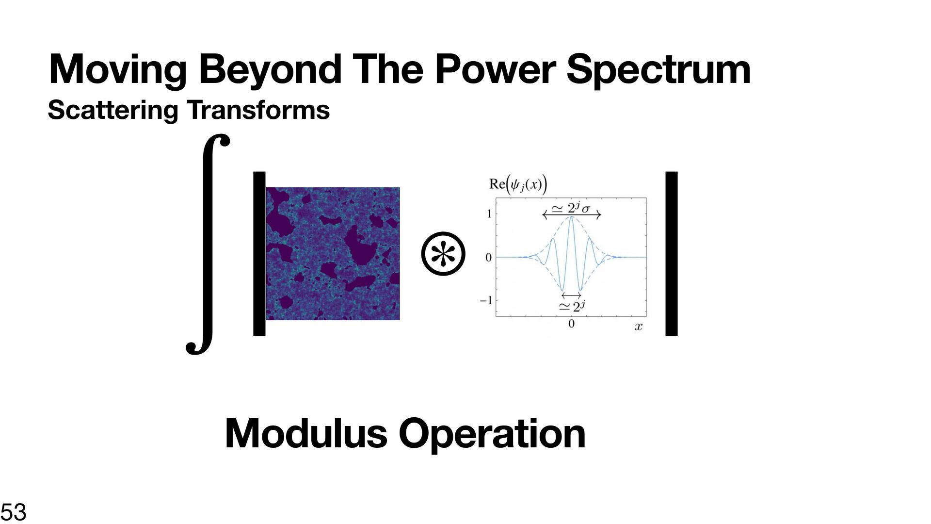
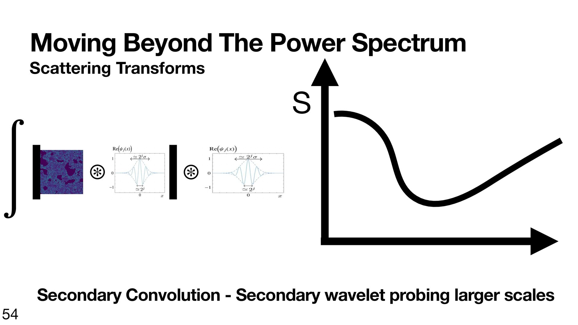
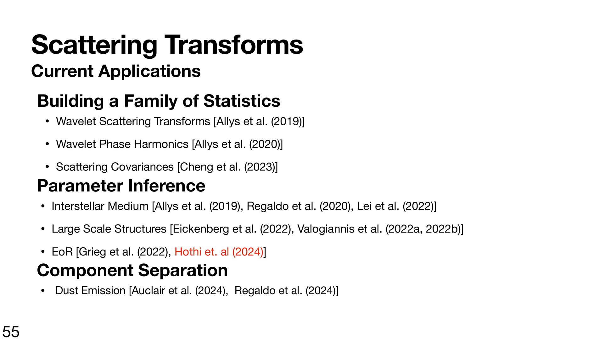
4. The Epoch of Reionization Why is it so important? • Sets the stage for the Universe we see today • The rst structures formed during this Epoch • The IGM, today, is ionized and it is during this period where the IGM went from neutral to ionized • ItÕs a 1 billion year epoch in the history of the Universe that we know little fi about 4
5. How to observe the EoR? 5
6. Indirect Constraints Constraints from Planck ¥Planck: Z_start≈14 ¥ 6
7. Indirect Constraints Constraints from Planck & The G-P Trough ¥Planck: Z_start≈14 ¥G-P Trough: Z_end≈6 ¥ 7
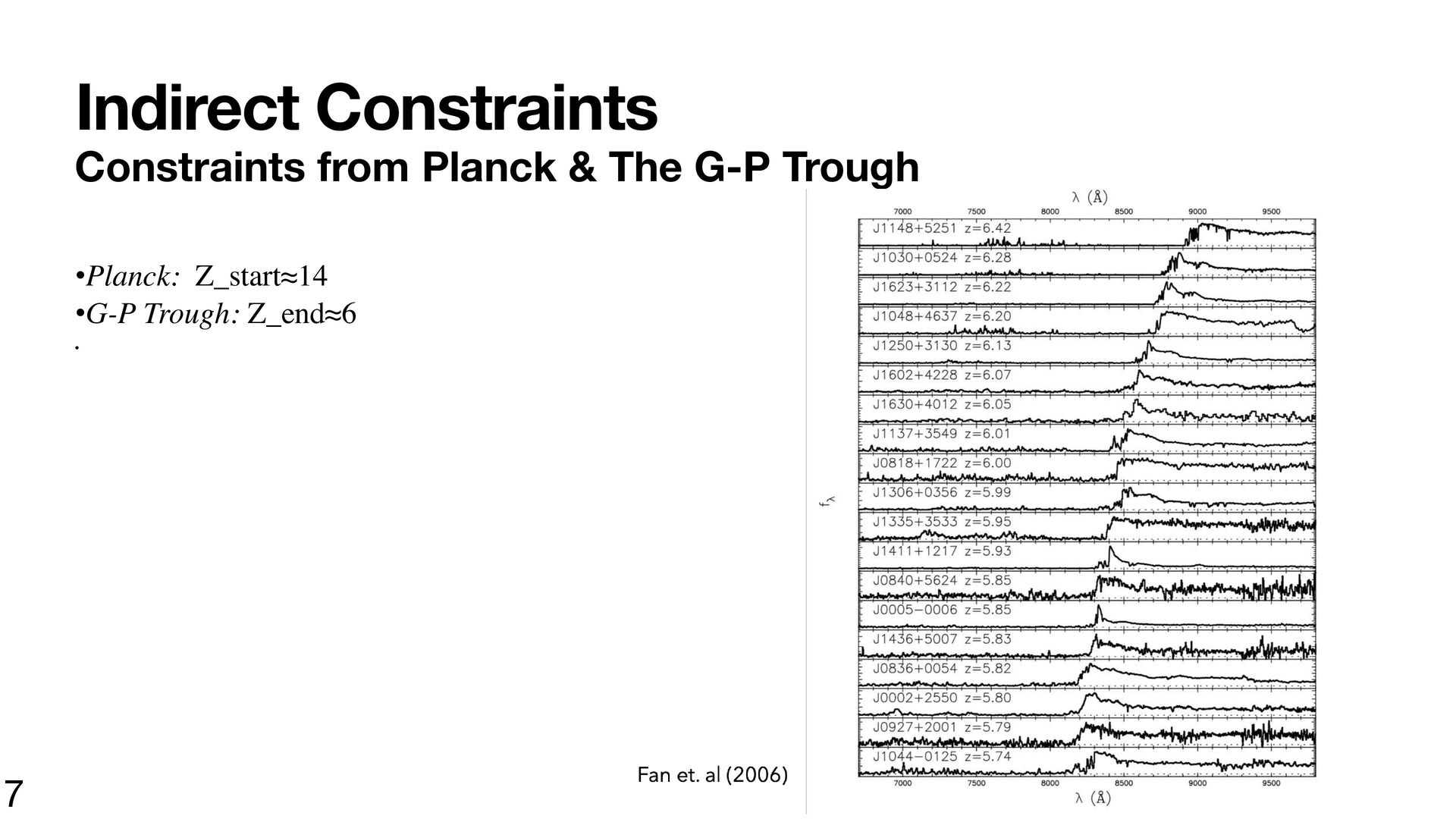
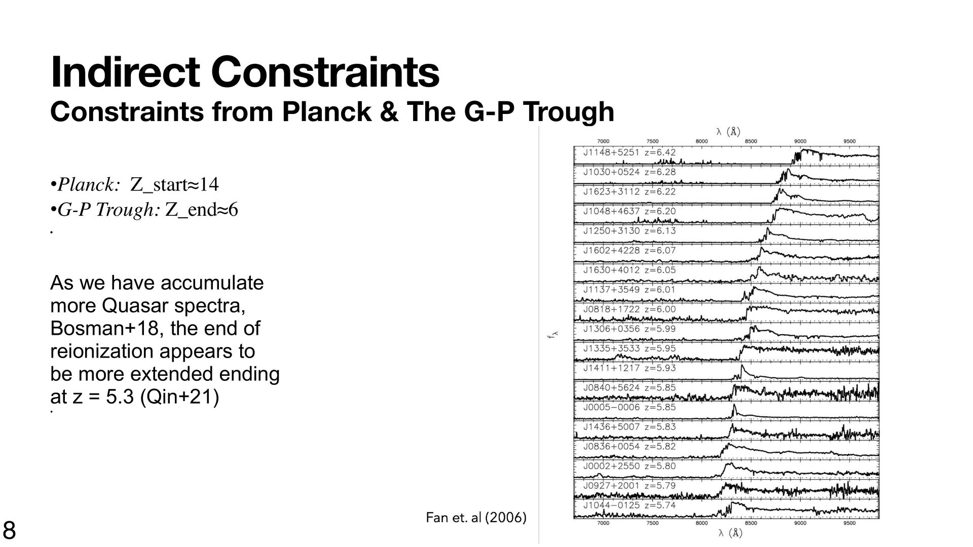
8. Indirect Constraints Constraints from Planck & The G-P Trough ¥Planck: Z_start≈14 ¥G-P Trough: Z_end≈6 ¥ As we have accumulate more Quasar spectra, Bosman+18, the end of reionization appears to be more extended ending at z = 5.3 (Qin+21) ¥ 8
9. Direct Constraints on the EoR 9
10. The 21cm Signal fi Hyper ne Transition Line of Hydrogen 10 Oyama (2015)
11. 11 The 21cm Signal A Probe of the IGM dIν = − Iν + Bν(ν) dτν
12. 12 The 21cm Signal A Probe of the IGM dIν = − Iν + Bν(ν) dτν 2 Iνc Tb(ν) ≈ 2 2kBν
13. 13 The 21cm Signal A Probe of the IGM dTb = − Tb + TCMB dτν
14. 14 The 21cm Signal A Probe of the IGM Tb(τν) = TS(1 − e −τν ) + TCMBe −τν TS = Tb(τν = 0)
15. The 21cm Signal A Probe of the IGM 2 TCMB Ωbh 0.24 H(z) 1+z δTb = 28(1 + δ)xHI 1 − ( TS )( 0.0223 ) ( Ωm )( 10 )[ δrvr + H(z) ] 15
16. The 21cm Signal A Probe of the IGM 2 TCMB Ωbh 0.24 H(z) 1+z δTb = 28(1 + δ)xHI 1 − ( TS )( 0.0223 ) ( Ωm )( 10 )[ δrvr + H(z) ] Matter Density 16
17. The 21cm Signal A Probe of the IGM 2 TCMB Ωbh 0.24 H(z) 1+z δTb = 28(1 + δ)xHI 1 − ( TS )( 0.0223 ) ( Ωm )( 10 )[ δrvr + H(z) ] Matter Density Neutral Fraction 17
18. The 21cm Signal A Probe of the IGM 2 TCMB Ωbh 0.24 H(z) 1+z δTb = 28(1 + δ)xHI 1 − ( TS )( 0.0223 ) ( Ωm )( 10 )[ δrvr + H(z) ] Matter Density Neutral Fraction Cosmology 18
19. 19 The 21cm Signal Timeline of Reionization Pritchard & Loeb (2011)
20. 20 How to Observe the EoR Radio Interferometry
21. 21 How to Observe the EoR Radio Interferometry
22. How to Observe the EoR Radio Interferometry 22
23. How to Observe the EoR Radio Interferometry 23
24. Radio Interferometers Active Collaborations LOFAR NenuFAR 24 HERA MWA
25. Radio Interferometers Future Experiments SKA 25
26. How to Observe the EoR Lightcones 26
27. How to Observe the EoR Lightcones 2D Sky Redsh ift/Fre 27 quenc y
28. How to Observe the EoR Towards a rst detection Current interferometers do not have the sensitivity to detect tomographic maps of the EoR fi They instead aim for a statistical detection of the EoR 28
29. How to Observe the EoR Power Spectrum 2D Sky Redsh ift/Fre 29 quenc y
30. How to Observe the EoR Power Spectrum ky kx kz 30
31. How to Observe the EoR Power Spectrum 2 ky kx kz 31
32. How to Observe the EoR Power Spectrum 2 ky kx kz 32
33. How to Observe the EoR Power Spectrum P(k) k k= 33 2 2 2 kx + ky + kz
34. Why HavenÕt Radio Interferometers Detected the EoR? 34
35. Detecting the EoR Foregrounds and Systematics 35
36. Detecting the EoR Foregrounds and Systematics 36 Jelić et al. (2008)
37. Detecting the EoR How to mitigate these contaminants? 37
38. Detecting the EoR How to mitigate these contaminants? Foreground Avoidance 38 Foreground Removal
39. Detecting the EoR How to mitigate these contaminants? Foreground Avoidance 2 ky kx kz 39
40. Detecting the EoR How to mitigate these contaminants? Foreground Avoidance k∥ = | kz | k⊥ = 40 2 2 kx + ky
41. Detecting the EoR How to mitigate these contaminants? Foreground Removal Observed Signal 21cm Signal 41 Jelić et al. (2008)
42. Detecting the EoR How to mitigate these contaminants? Foreground Avoidance Foreground Removal k∥ = | kz | 42 k⊥ = 2 2 kx + ky Jelić et al. (2008)
43. Detecting the EoR Power Spectrum Upper Limits 43 Courtesy of Florent Mertens
44. Detecting the EoR What are the current limitations? 44
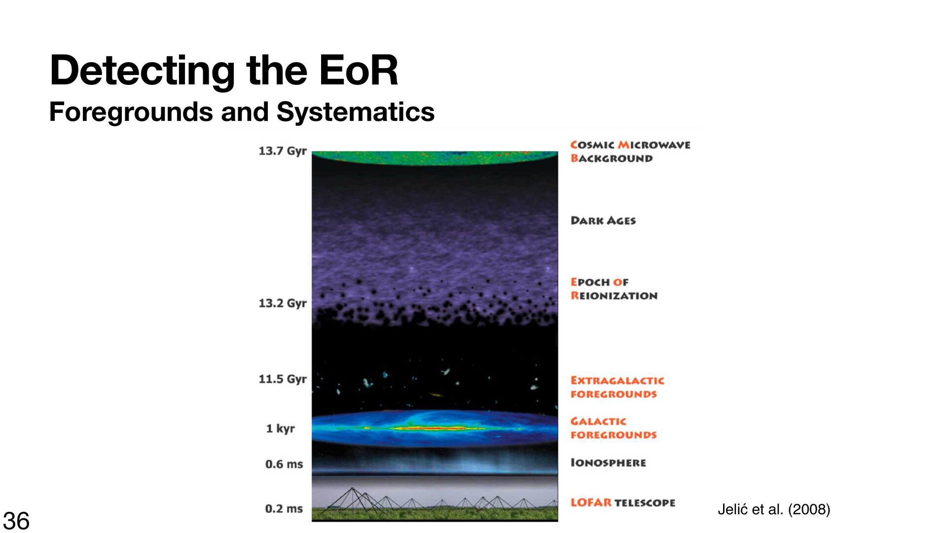
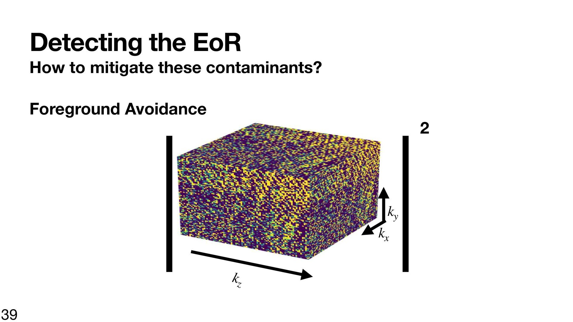
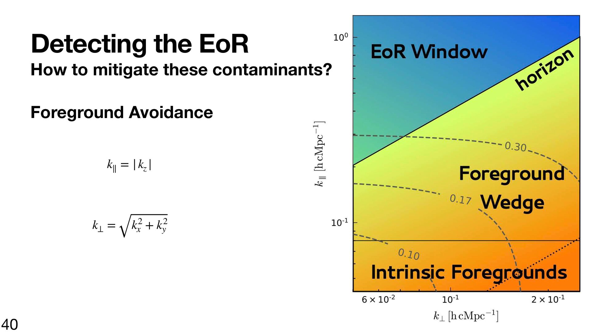
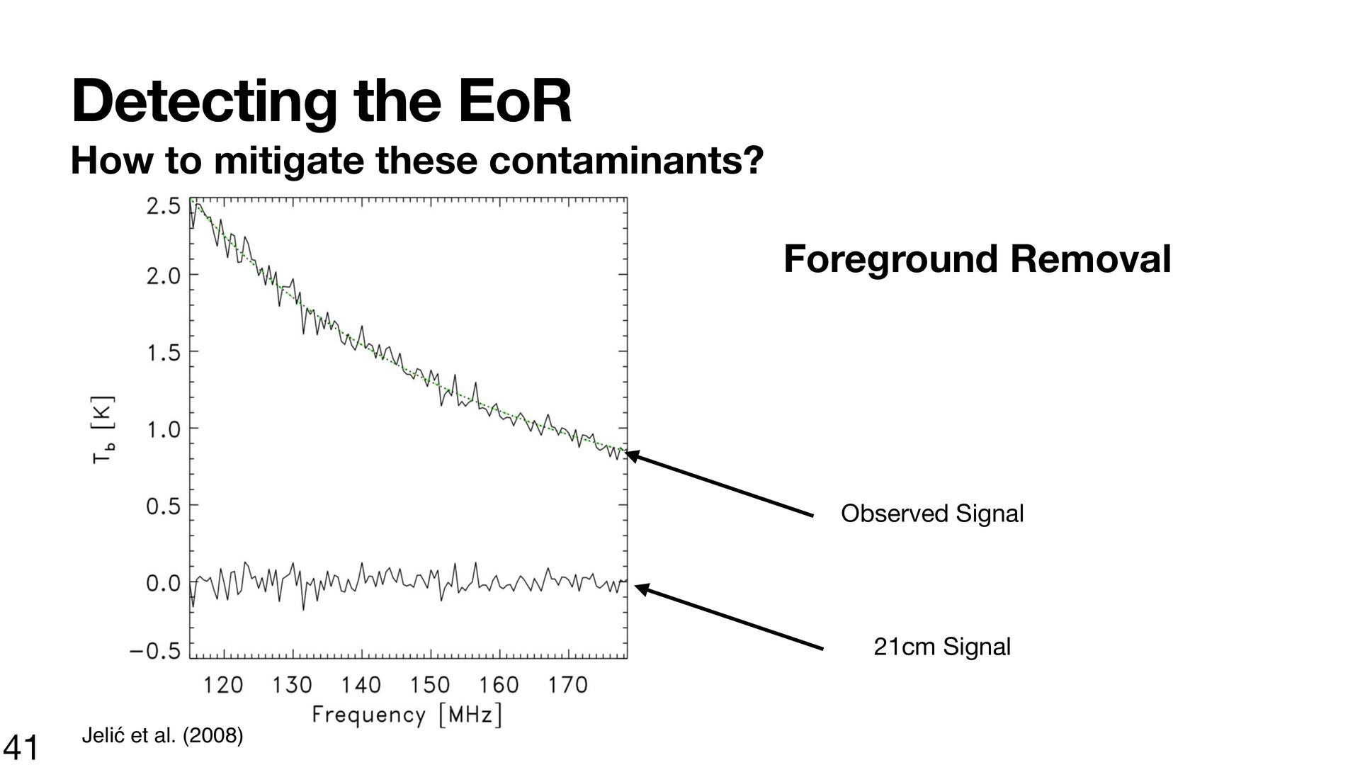
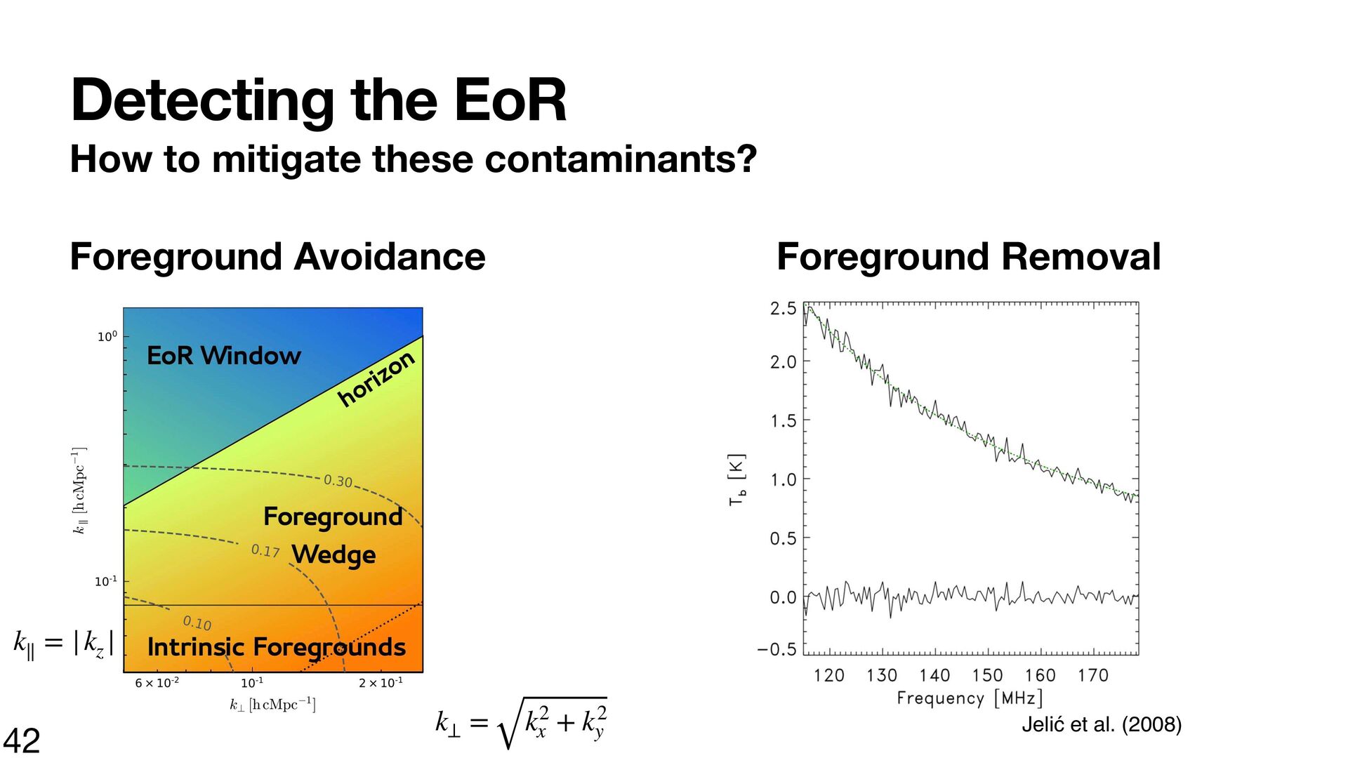
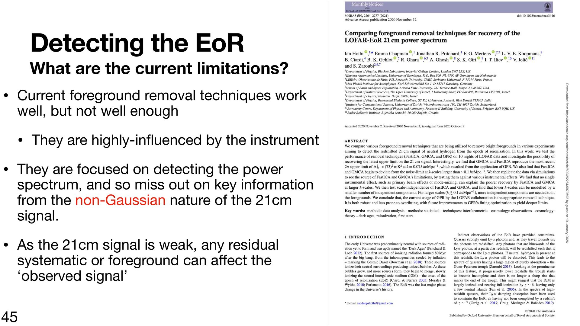
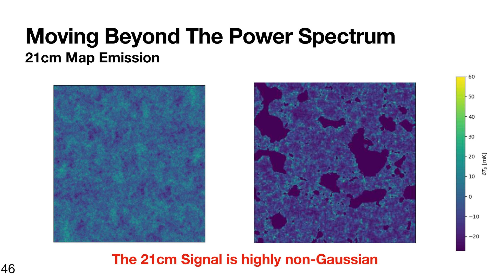
45. Detecting the EoR What are the current limitations? • Current foreground removal techniques work well, but not well enough • They are highly-in uenced by the instrument • They are focused on detecting the power spectrum, and so miss out on key information from the non-Gaussian nature of the 21cm signal. • As the 21cm signal is weak, any residual 45 ff fl systematic or foreground can a ect the Ôobserved signalÕ
46. Moving Beyond The Power Spectrum 21cm Map Emission 46 The 21cm Signal is highly non-Gaussian
47. Moving Beyond The Power Spectrum The Bispectrum Hutter et al. (2019) 47
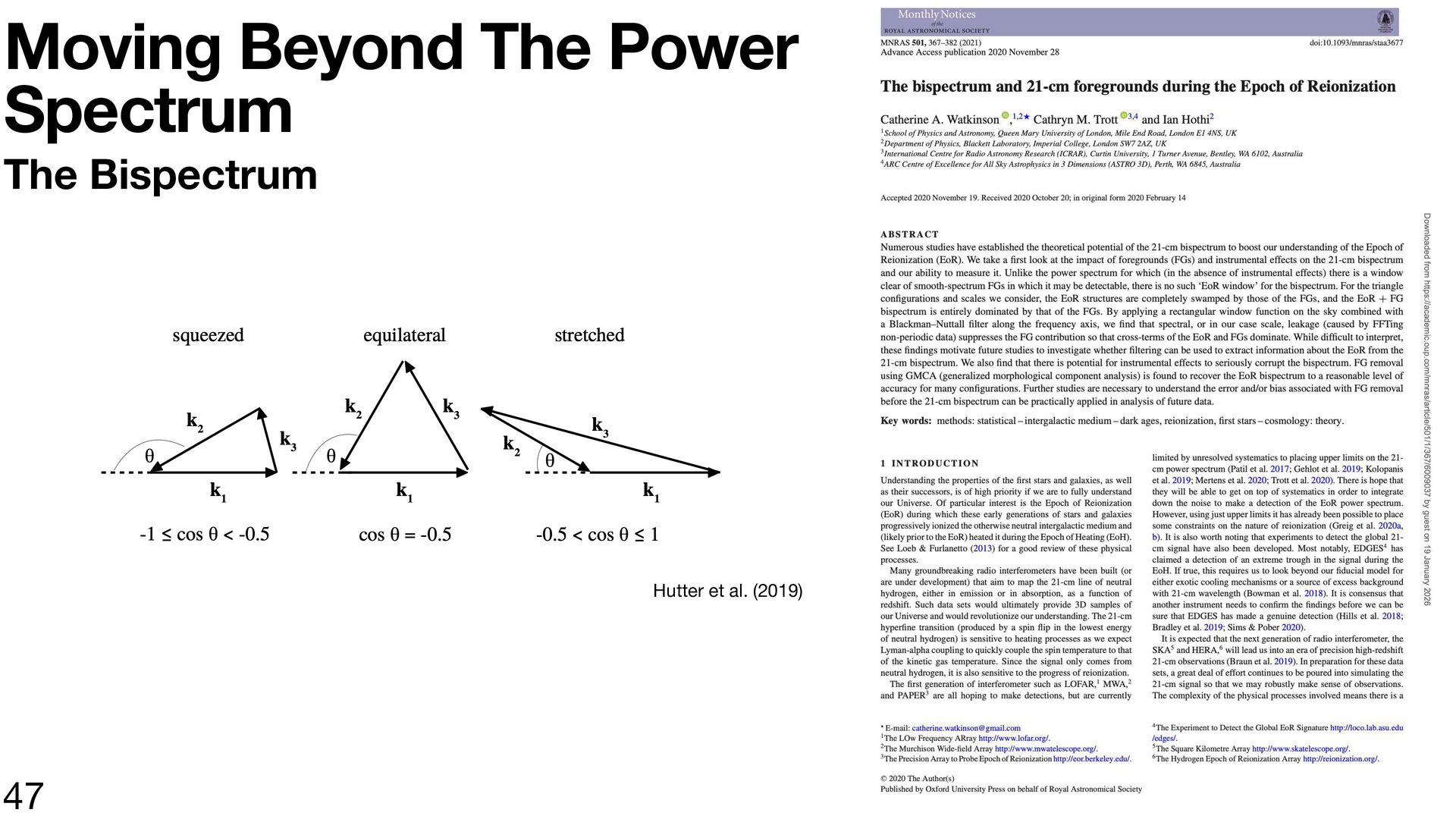
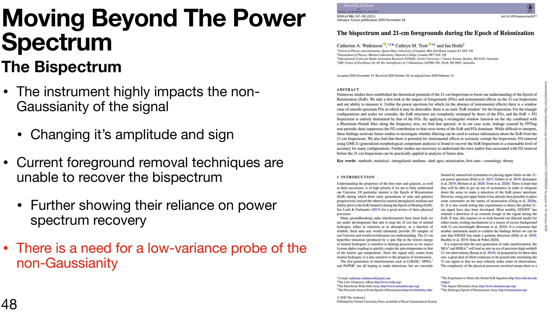
48. Moving Beyond The Power Spectrum The Bispectrum • The instrument highly impacts the nonGaussianity of the signal • Changing itÕs amplitude and sign • Current foreground removal techniques are unable to recover the bispectrum • Further showing their reliance on power spectrum recovery • There is a need for a low-variance probe of the non-Gaussianity 48
49. Moving Beyond The Power Spectrum Scattering Transforms 49
50. Moving Beyond The Power Spectrum Scattering Transforms 21cm Emission Map 50
51. Moving Beyond The Power Spectrum Scattering Transforms ⊛ Wavelet Convolution 51
52. Moving Beyond The Power Spectrum Scattering Transforms ⊛ 52
53. Moving Beyond The Power Spectrum Scattering Transforms ∫ ⊛ Modulus Operation 53
54. Moving Beyond The Power Spectrum Scattering Transforms ∫ S + ⊛ ⊛ + Secondary Convolution - Secondary wavelet probing larger scales 54
55. Scattering Transforms Current Applications Building a Family of Statistics • Wavelet Scattering Transforms [Allys et al. (2019)] • Wavelet Phase Harmonics [Allys et al. (2020)] • Scattering Covariances [Cheng et al. (2023)] Parameter Inference • Interstellar Medium [Allys et al. (2019), Regaldo et al. (2020), Lei et al. (2022)] • Large Scale Structures [Eickenberg et al. (2022), Valogiannis et al. (2022a, 2022b)] • EoR [Grieg et al. (2022), Hothi et. al (2024)] Component Separation • Dust Emission [Auclair et al. (2024), Regaldo et al. (2024)] 55
56. Scattering Transforms Component Separation 56
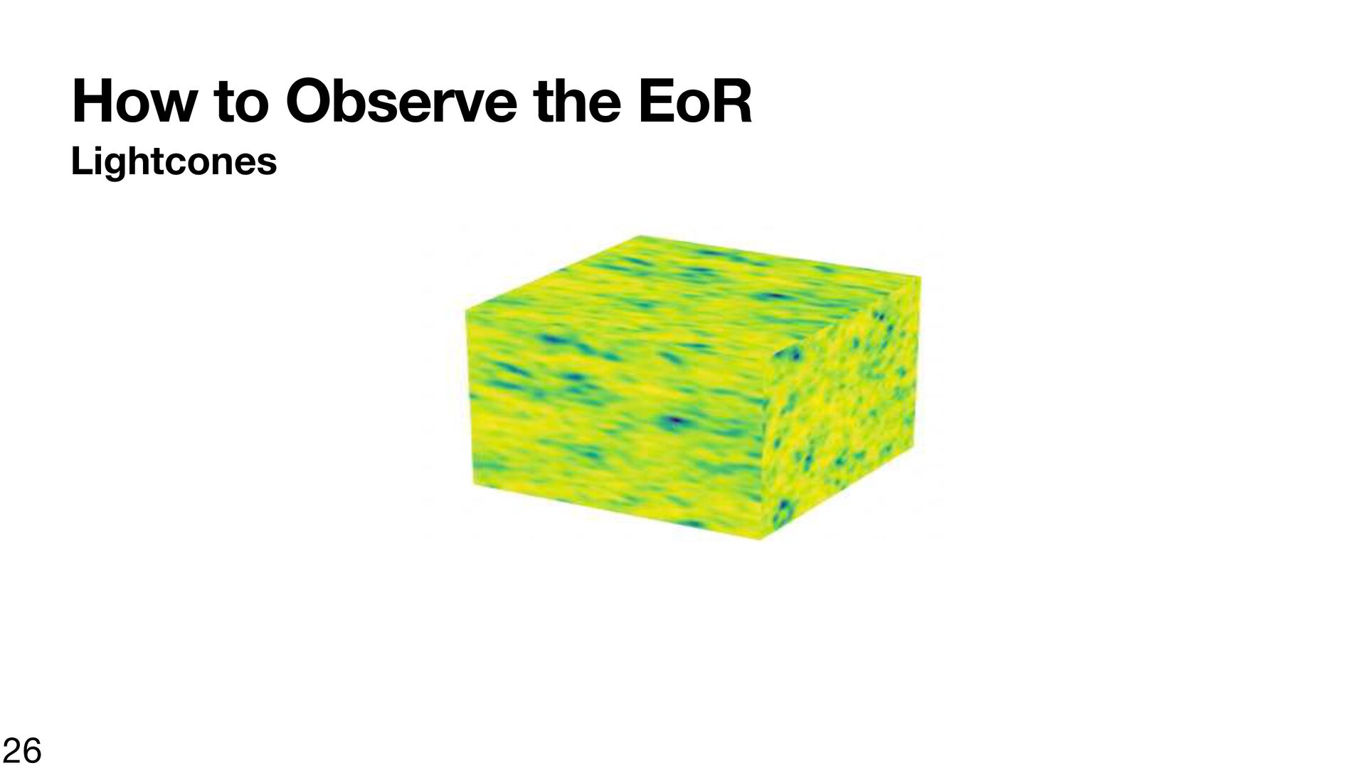
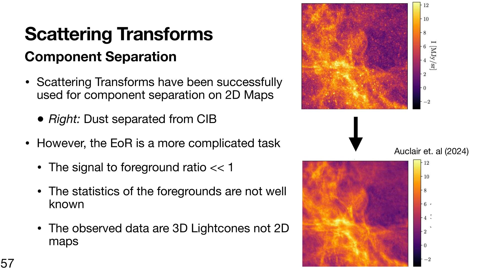
57. Scattering Transforms Component Separation • Scattering Transforms have been successfully used for component separation on 2D Maps ¥ Right: Dust separated from CIB • However, the EoR is a more complicated task • The signal to foreground ratio << 1 • The statistics of the foregrounds are not well known • The observed data are 3D Lightcones not 2D maps 57 Auclair et. al (2024)
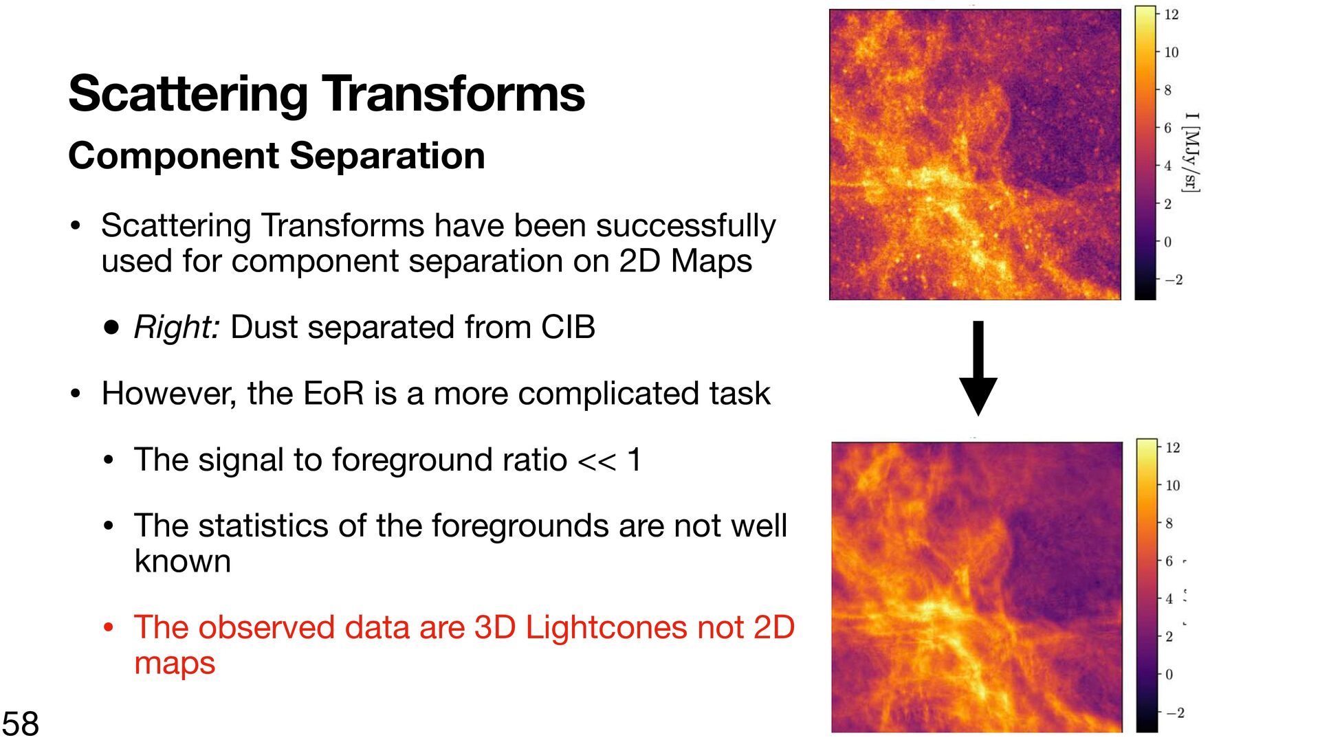
58. Scattering Transforms Component Separation • Scattering Transforms have been successfully used for component separation on 2D Maps ¥ Right: Dust separated from CIB • However, the EoR is a more complicated task • The signal to foreground ratio << 1 • The statistics of the foregrounds are not well known • The observed data are 3D Lightcones not 2D maps 58
59. Developing 3D Scattering Transform The EoR Problem 59
60. Developing 3D Scattering Transform The EoR Problem 60
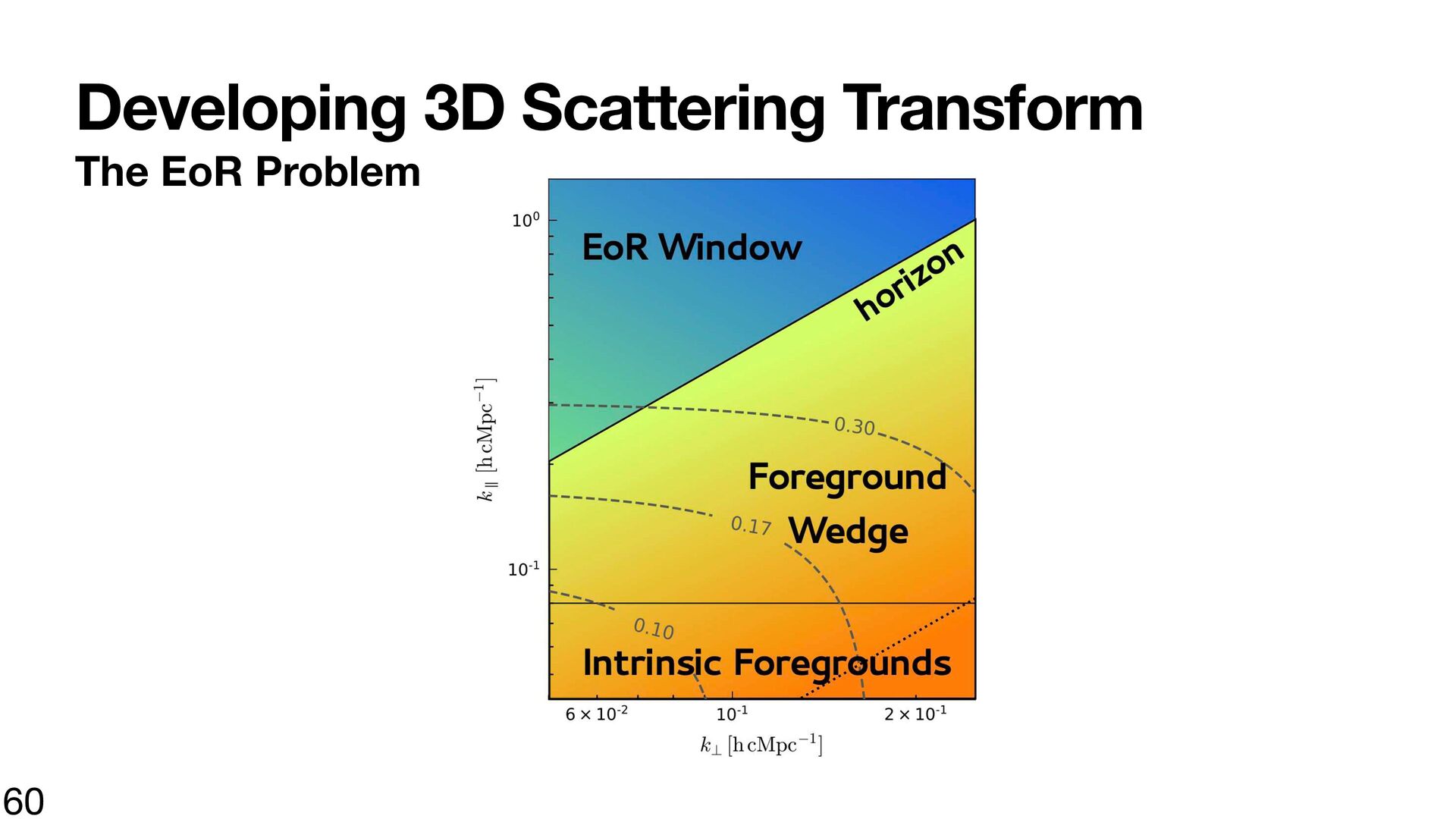
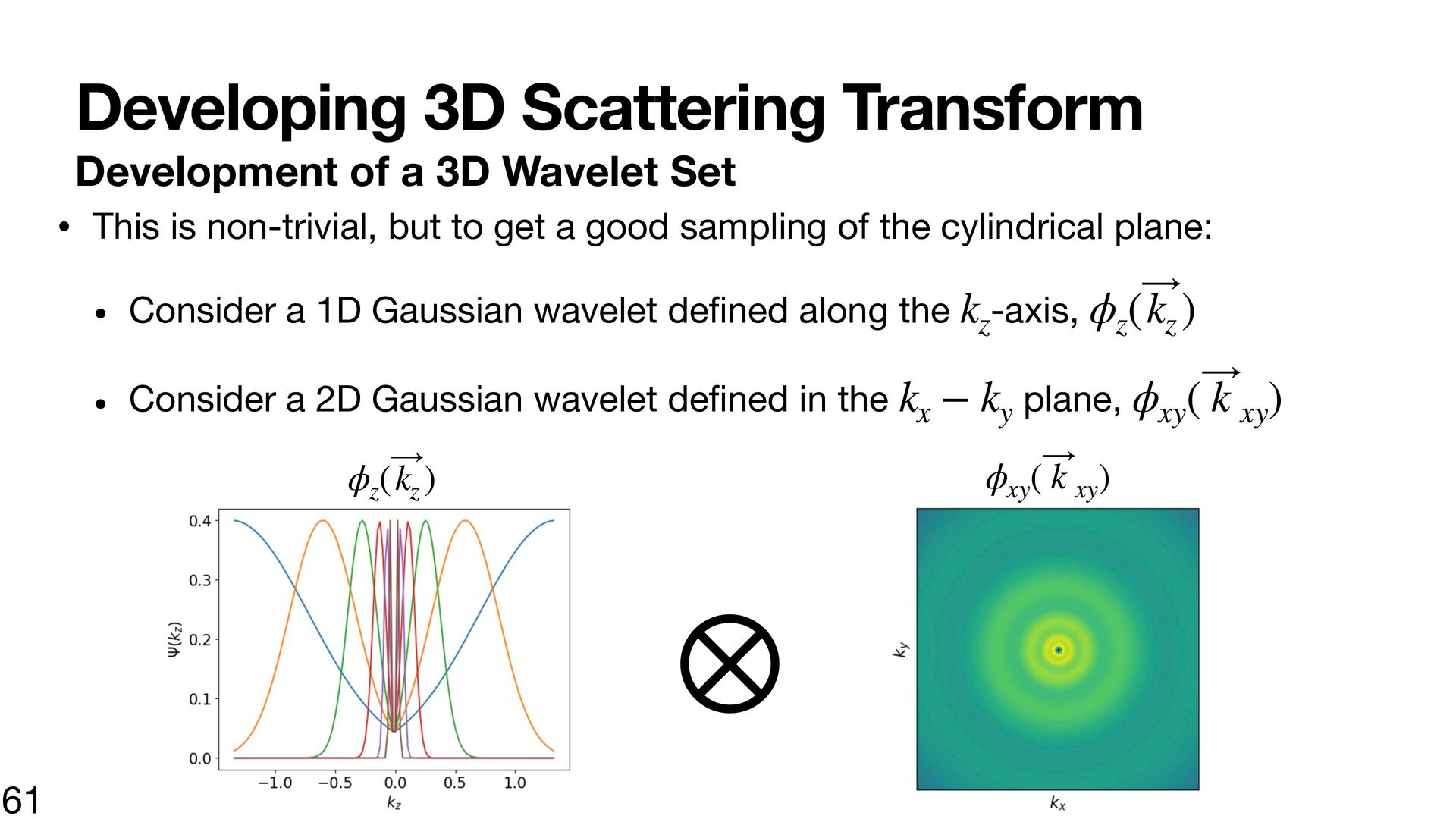
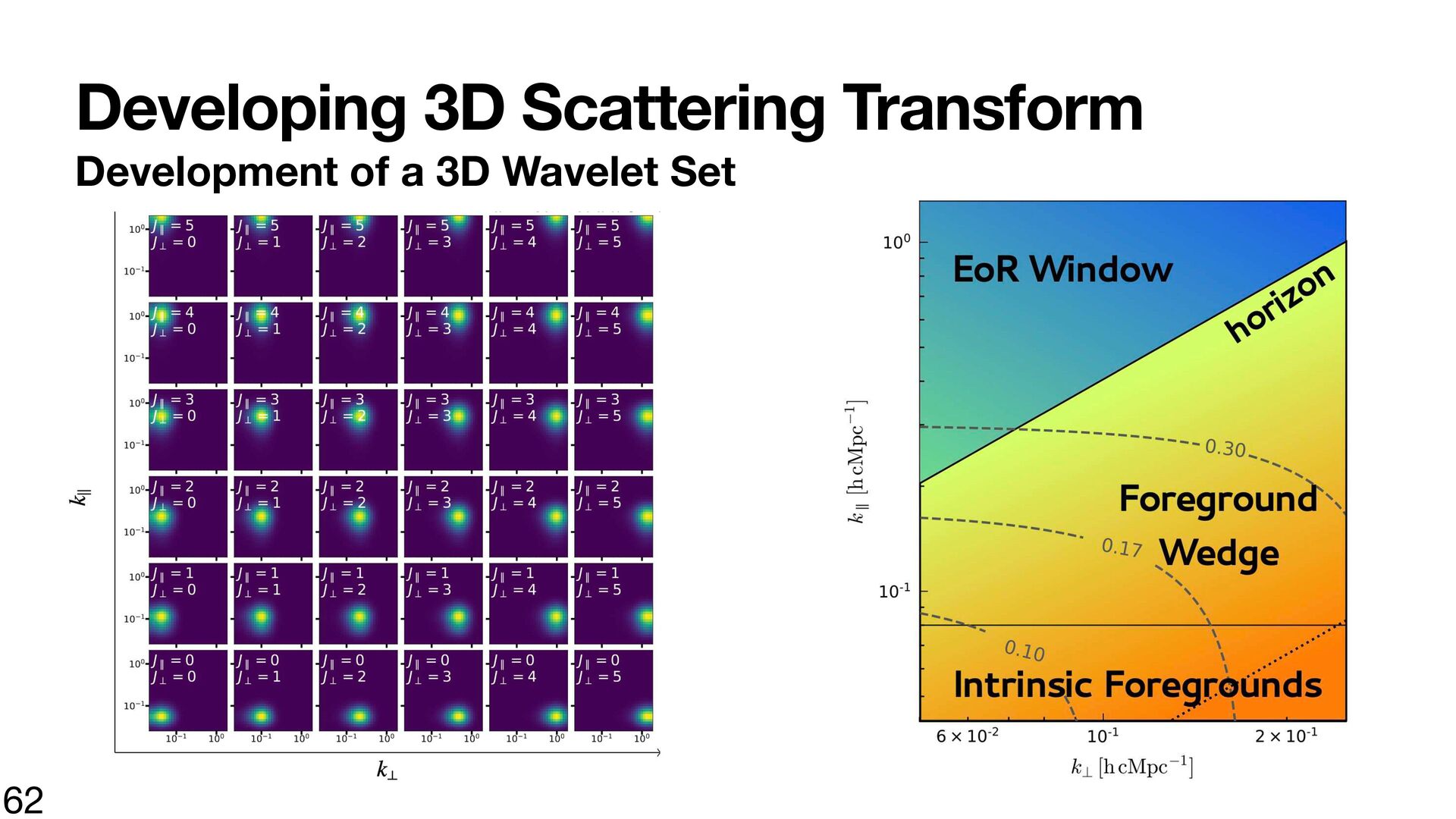
61. Developing 3D Scattering Transform Development of a 3D Wavelet Set • This is non-trivial, but to get a good sampling of the cylindrical plane: ⃗ • Consider a 1D Gaussian wavelet de ned along the k -axis, ϕ ( k ) z z z ⃗ • Consider a 2D Gaussian wavelet de ned in the k − k plane, ϕ ( k ) x ϕ ( k ⃗) z z fi fi ⨂ 61 y ⃗ ) ϕxy( k xy xy xy
62. Developing 3D Scattering Transform Development of a 3D Wavelet Set 62
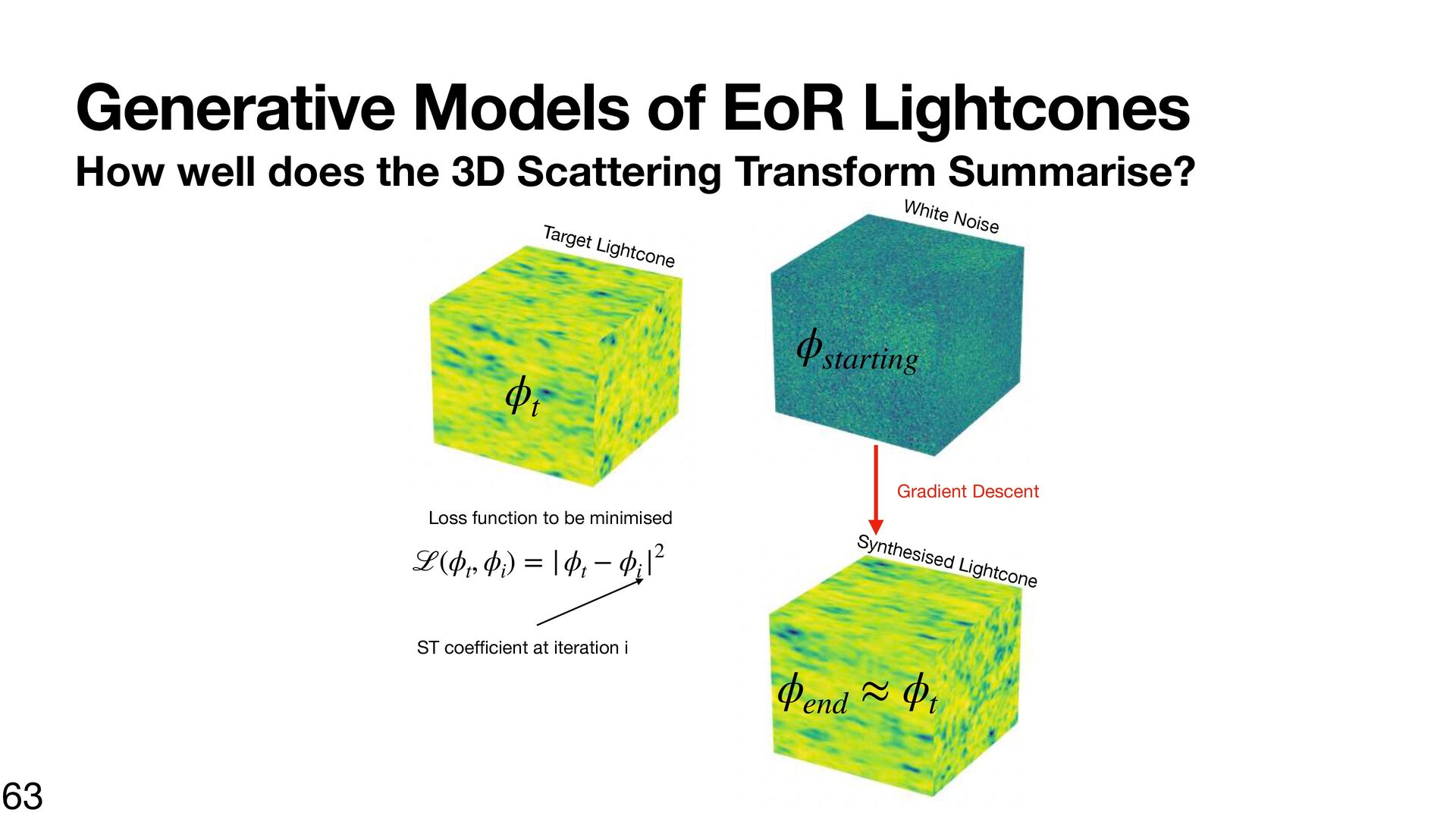
63. Generative Models of EoR Lightcones How well does the 3D Scattering Transform Summarise? White Targe t Noise Light cone ϕstarting ϕt Gradient Descent Loss function to be minimised 2 ℒ(ϕt, ϕi) = | ϕt − ϕi | Synth esise ST coe cient at iteration i 63 ffi ϕend ≈ ϕt d Lig htcon e
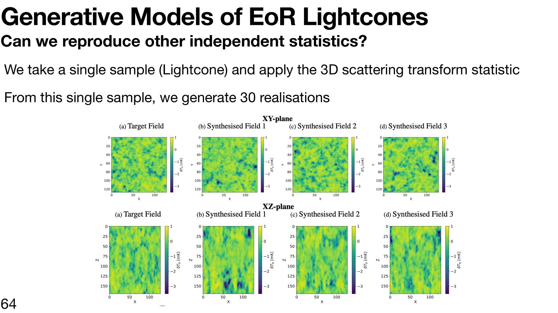
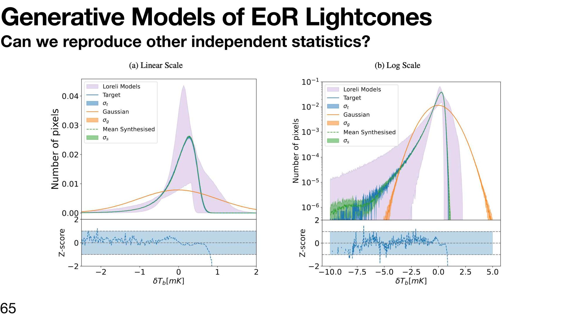
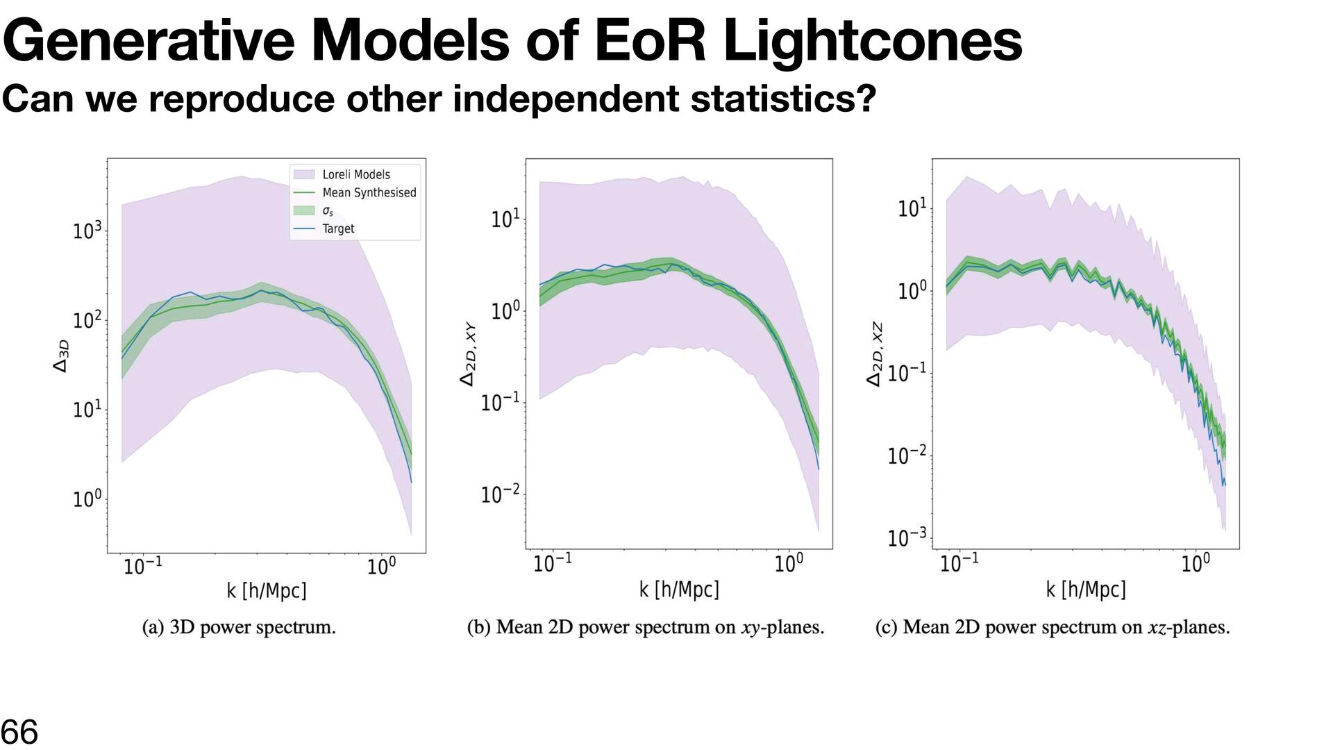
64. Generative Models of EoR Lightcones Can we reproduce other independent statistics? We take a single sample (Lightcone) and apply the 3D scattering transform statistic From this single sample, we generate 30 realisations 64
65. Generative Models of EoR Lightcones Can we reproduce other independent statistics? 65
66. Generative Models of EoR Lightcones Can we reproduce other independent statistics? 66
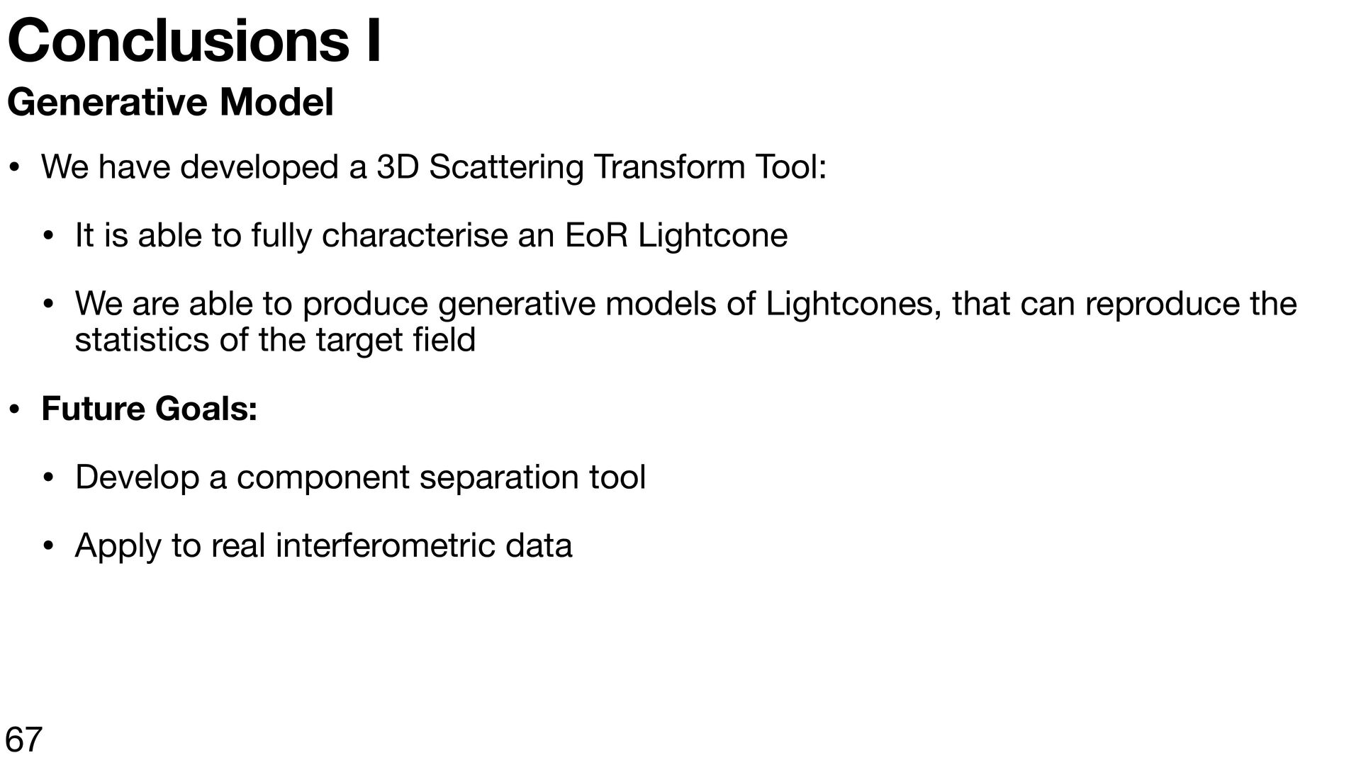
67. Conclusions I Generative Model • We have developed a 3D Scattering Transform Tool: • It is able to fully characterise an EoR Lightcone • We are able to produce generative models of Lightcones, that can reproduce the statistics of the target eld • Future Goals: • Develop a component separation tool fi • Apply to real interferometric data 67
68. Parameter Inference Post-Detection Constraints
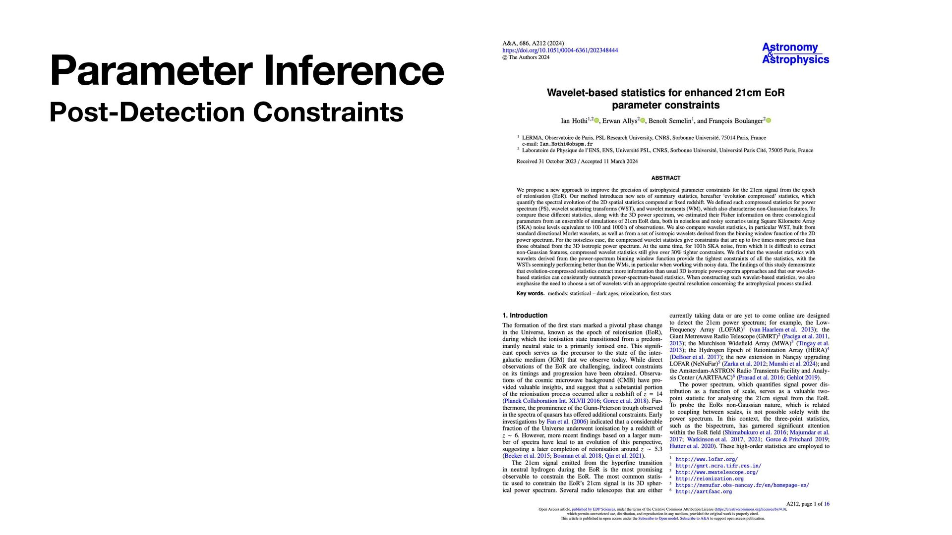
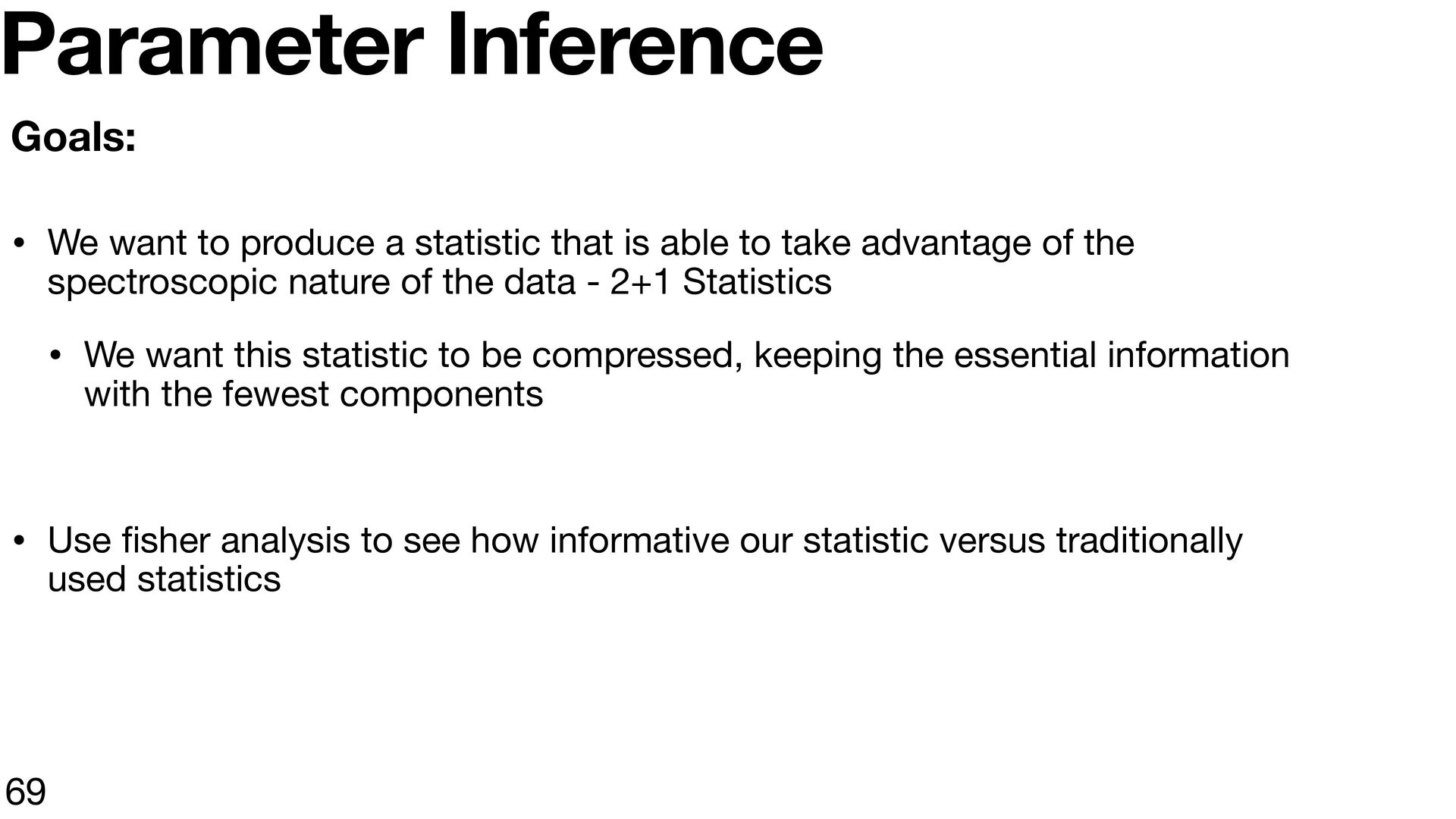
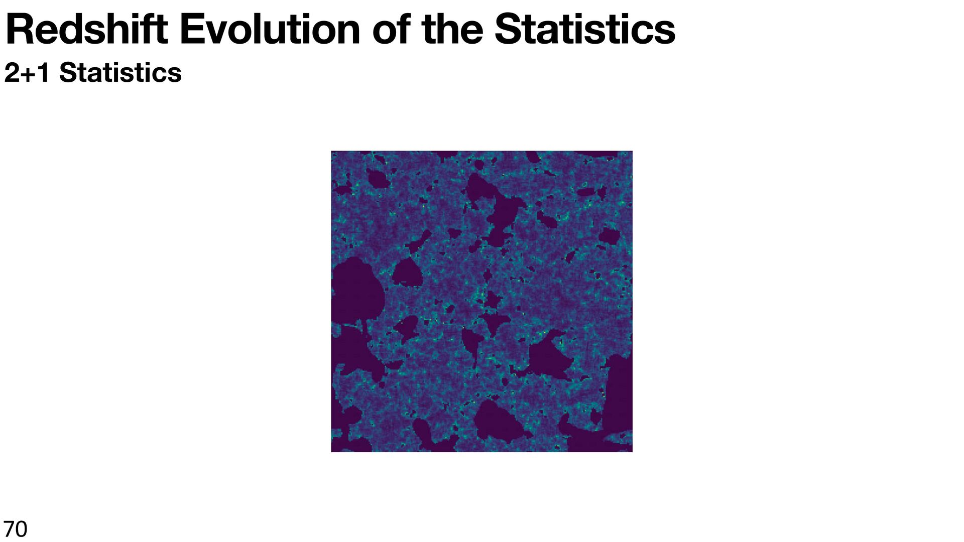
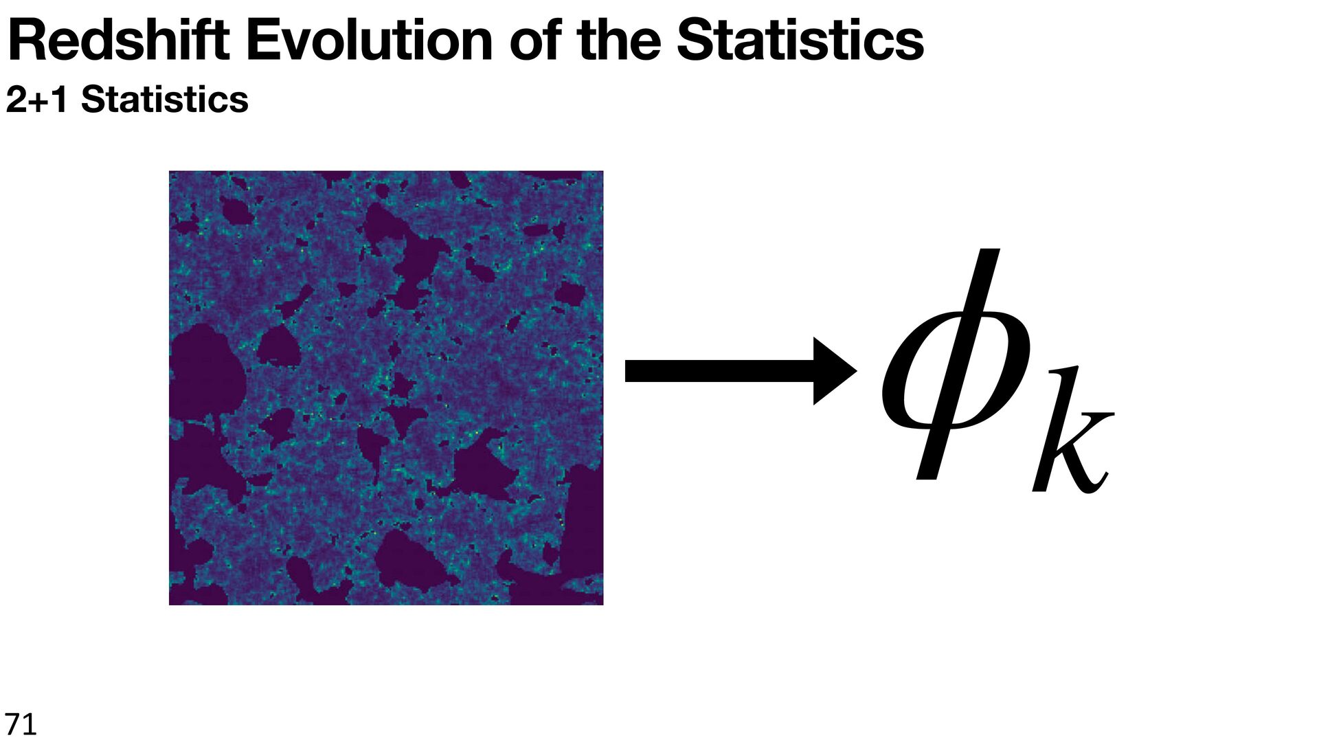
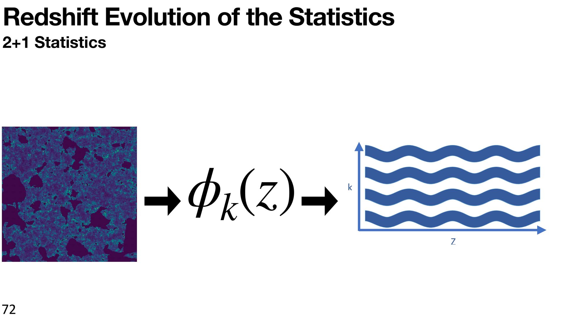
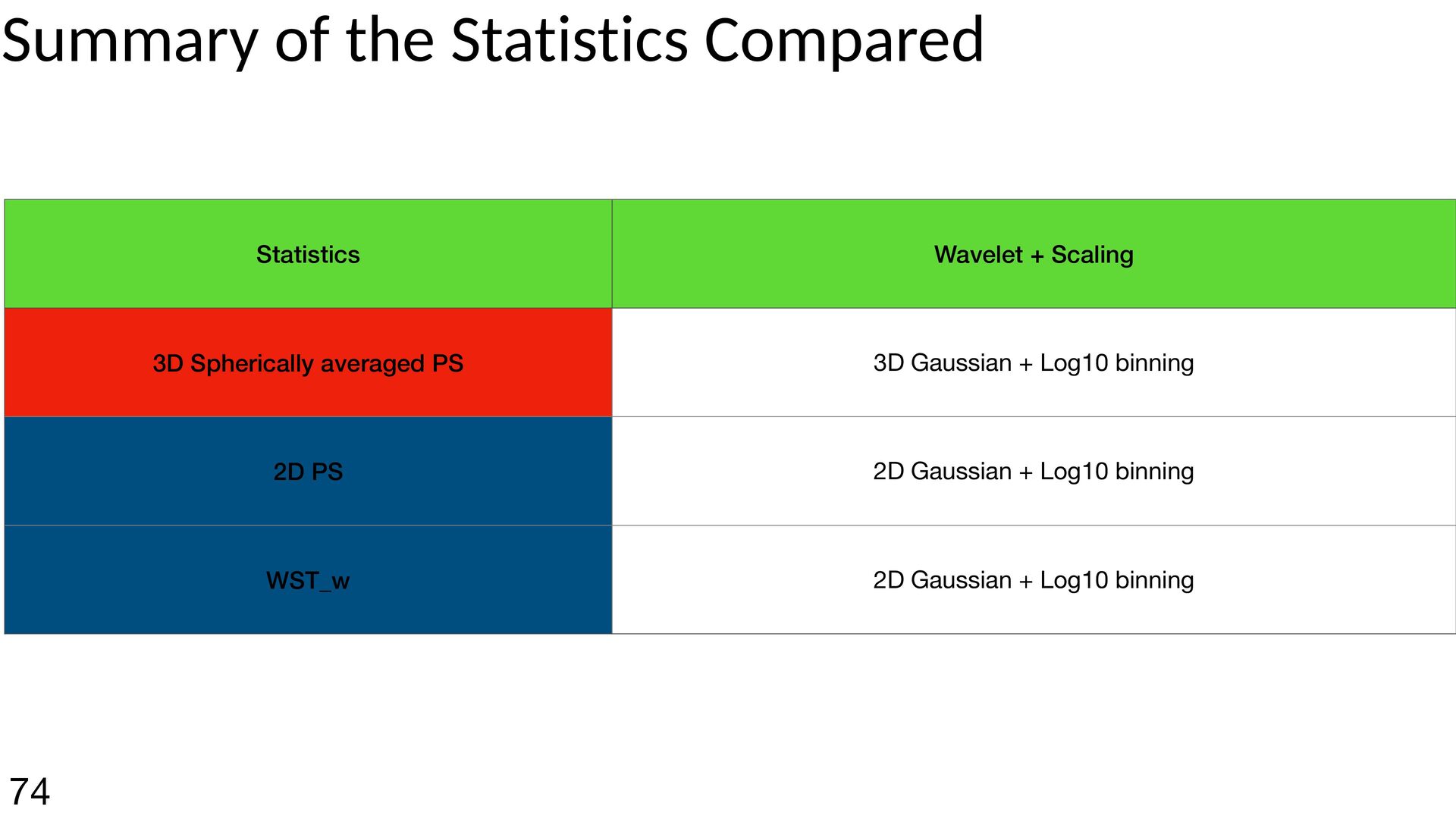
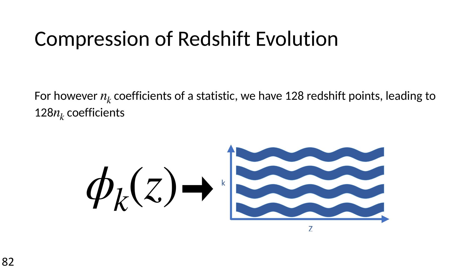
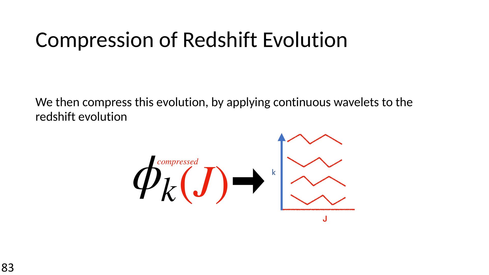
69. Parameter Inference Goals: • We want to produce a statistic that is able to take advantage of the spectroscopic nature of the data - 2+1 Statistics • We want this statistic to be compressed, keeping the essential information with the fewest components • Use sher analysis to see how informative our statistic versus traditionally used statistics fi 69
70. Redshift Evolution of the Statistics 2+1 Statistics 70
71. Redshift Evolution of the Statistics 2+1 Statistics ϕk 71
72. Redshift Evolution of the Statistics 2+1 Statistics ϕk(z) k Z 72
73. Comparison of statistics 73
74. Summary of the Statistics Compared 74 Statistics Wavelet + Scaling 3D Spherically averaged PS 3D Gaussian + Log10 binning 2D PS 2D Gaussian + Log10 binning WST_w 2D Gaussian + Log10 binning
75. How will we compare them 75
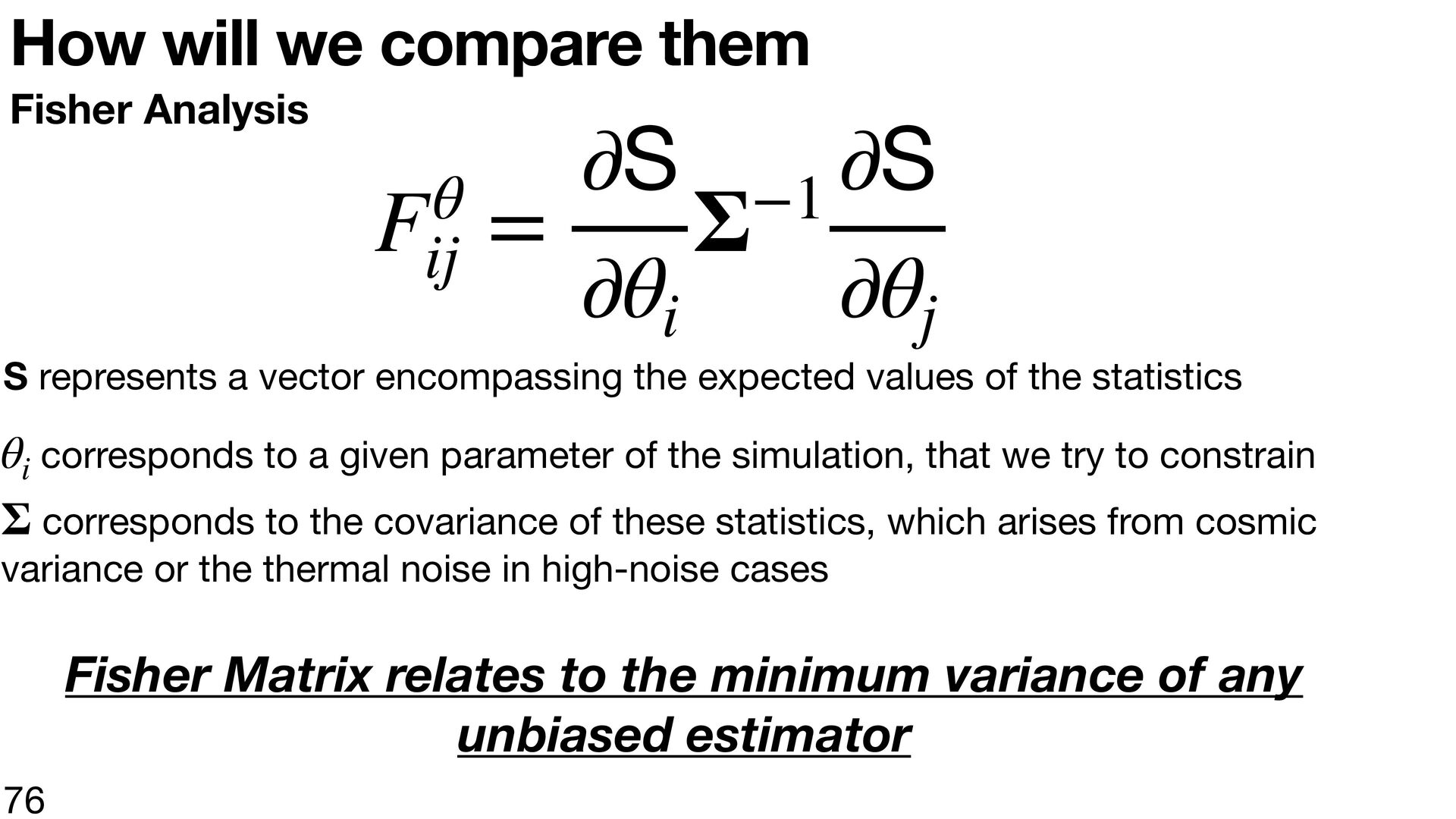
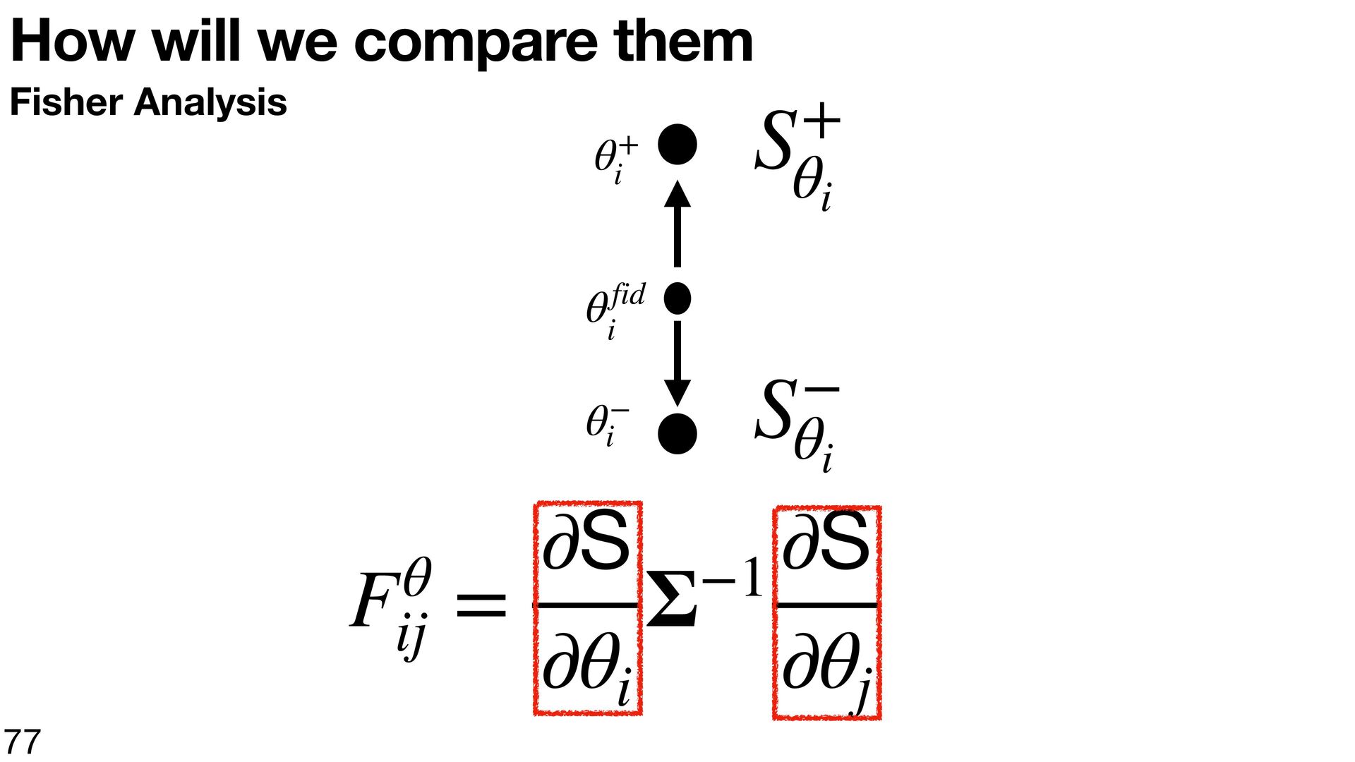
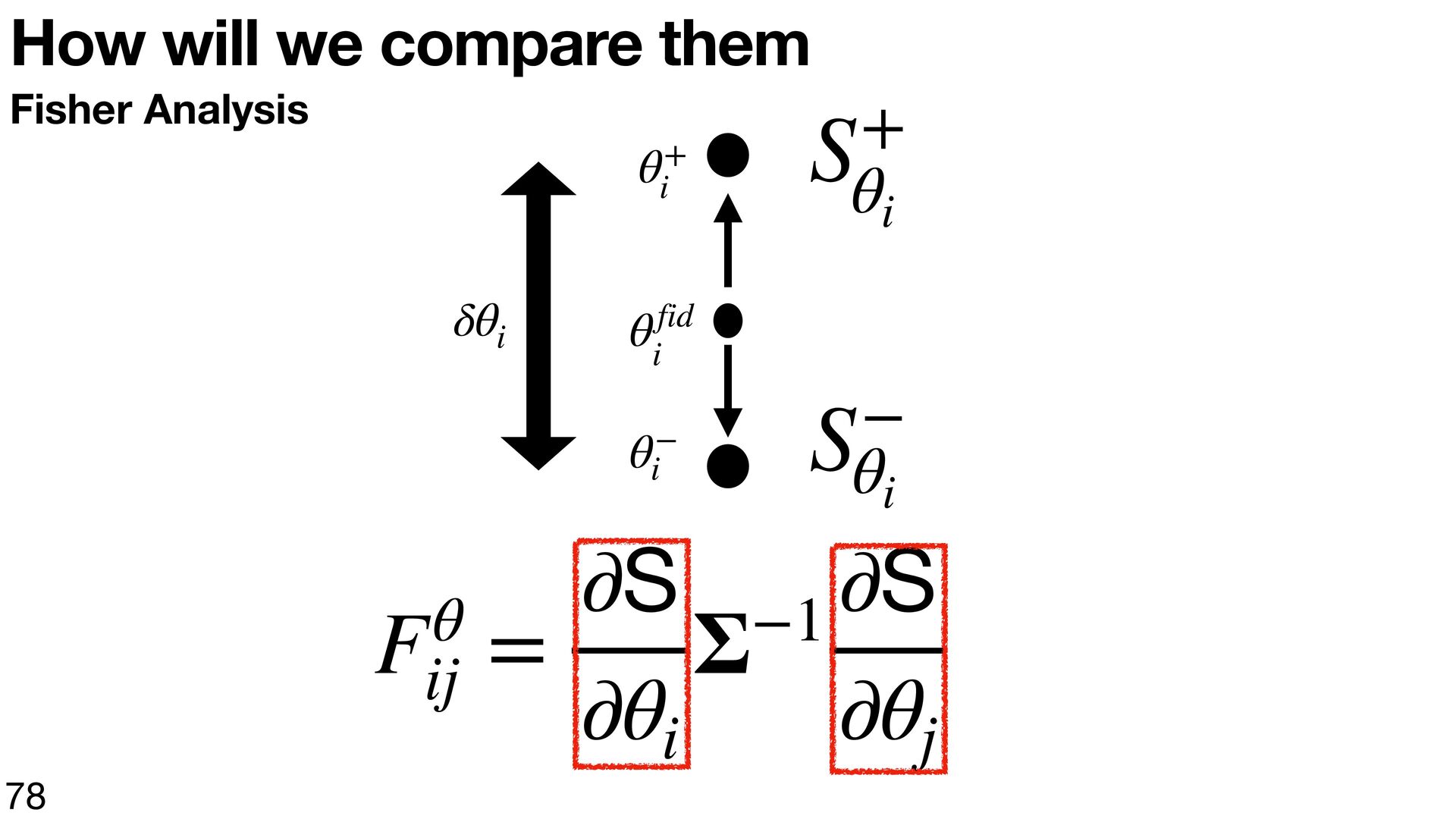
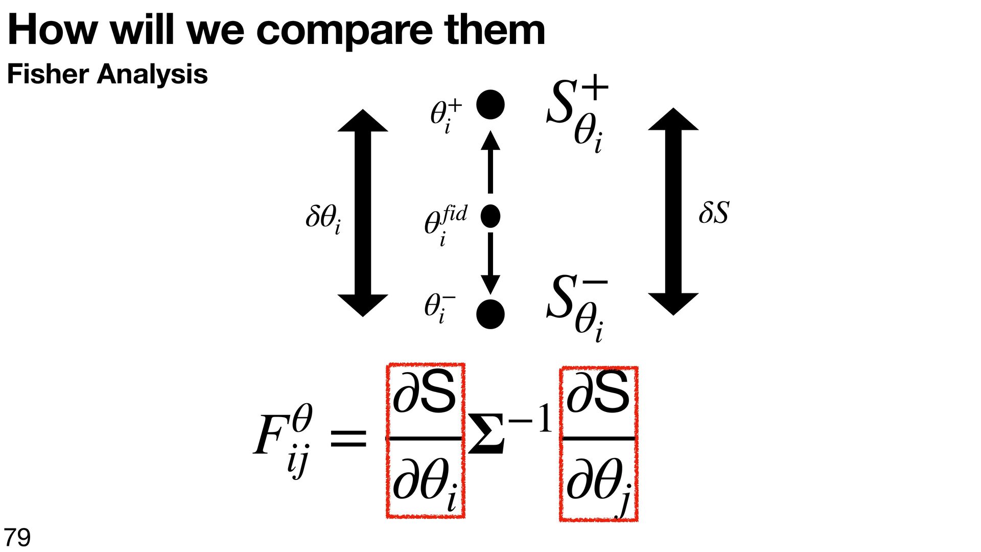
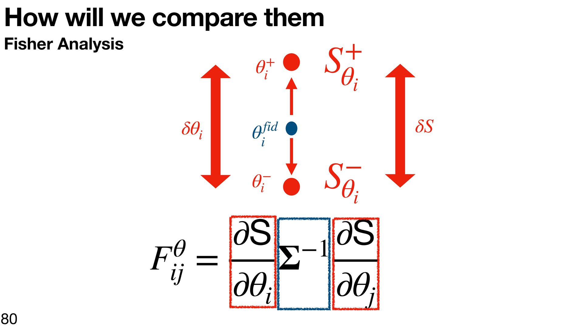
76. How will we compare them Fisher Analysis ∂S ∂S −1 θ Σ Fij = ∂θi ∂θj S represents a vector encompassing the expected values of the statistics θi corresponds to a given parameter of the simulation, that we try to constrain Σ corresponds to the covariance of these statistics, which arises from cosmic variance or the thermal noise in high-noise cases Fisher Matrix relates to the minimum variance of any unbiased estimator 76
77. How will we compare them Fisher Analysis + θi + Sθi fid θi − θi − Sθi ∂S ∂S −1 θ Σ Fij = ∂θi ∂θj 77
78. How will we compare them Fisher Analysis + θi δθi + Sθi fid θi − θi − Sθi ∂S ∂S −1 θ Σ Fij = ∂θi ∂θj 78
79. How will we compare them Fisher Analysis + θi δθi + Sθi δS fid θi − θi − Sθi ∂S ∂S −1 θ Σ Fij = ∂θi ∂θj 79
80. How will we compare them Fisher Analysis + θi δθi + Sθi δS fid θi − θi − Sθi ∂S ∂S −1 θ Σ Fij = ∂θi ∂θj 80
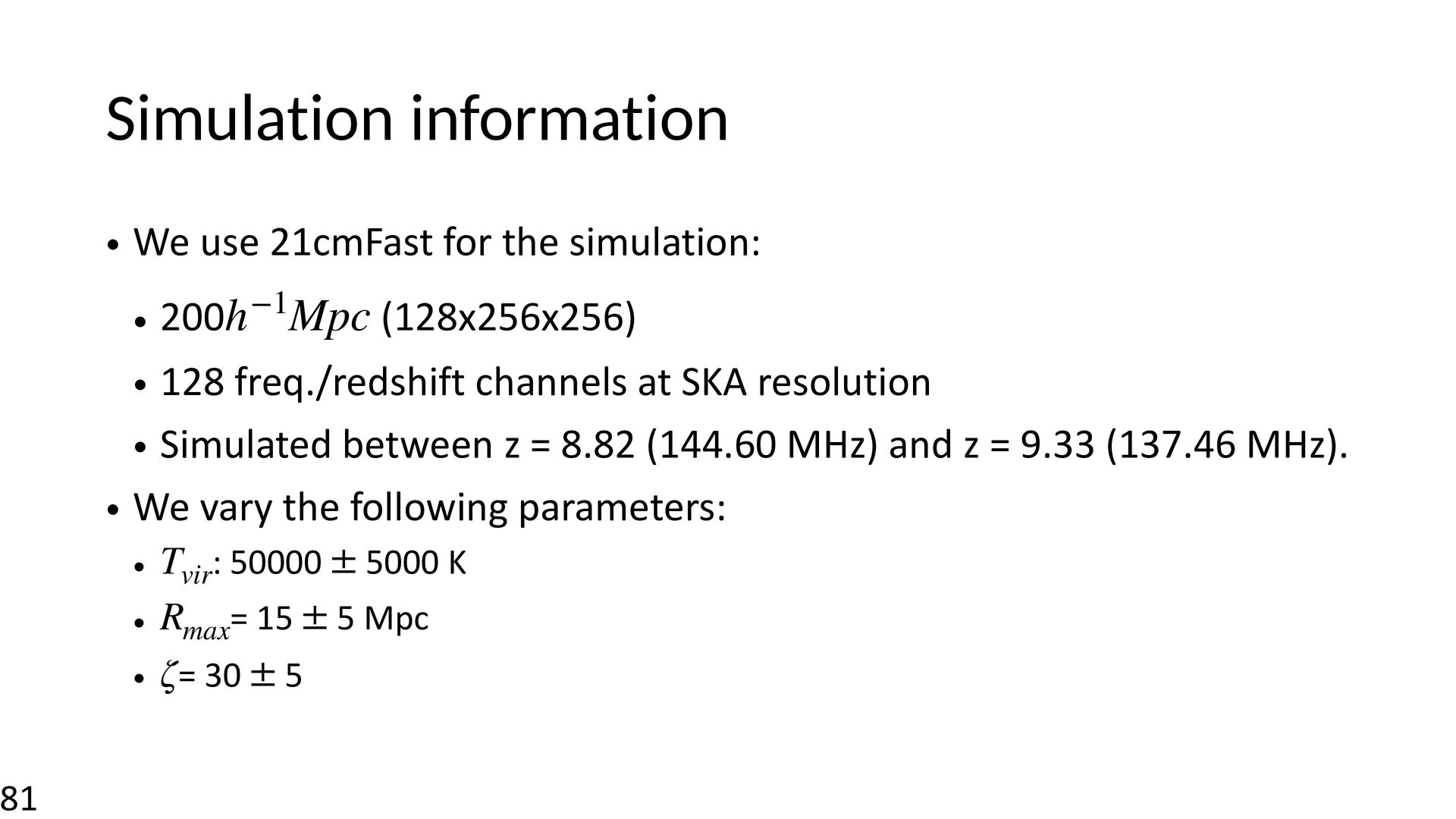
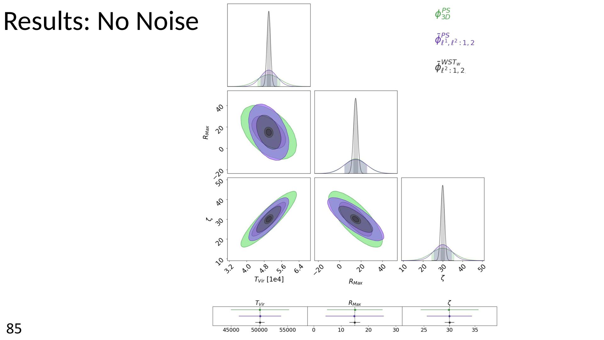
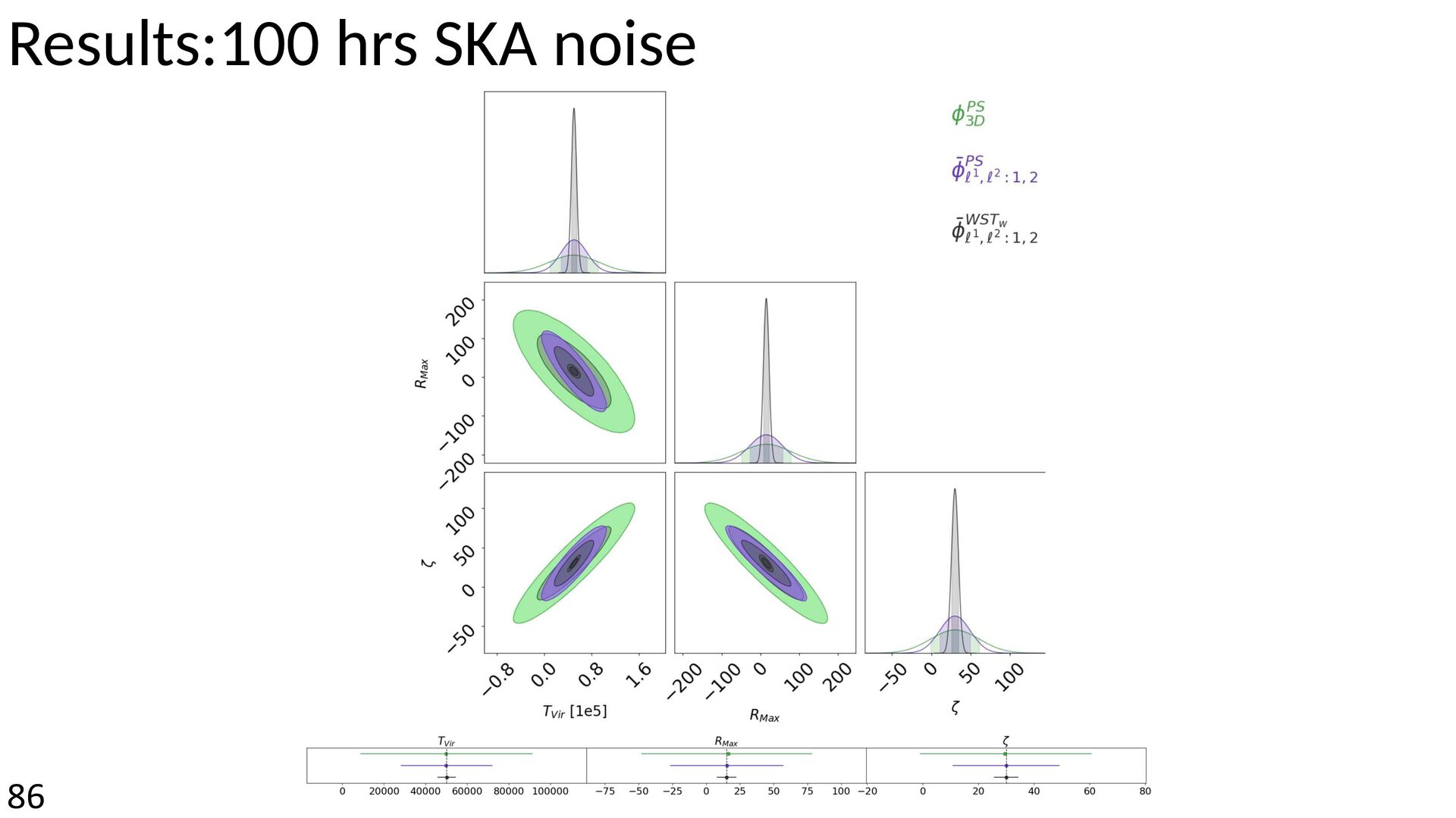
81. 81 Simulation information ¥ We use 21cmFast for the simulation: −1 ¥ 200h Mpc (128x256x256) ¥ 128 freq./redshift channels at SKA resolution ¥ Simulated between z = 8.82 (144.60 MHz) and z = 9.33 (137.46 MHz). ¥ We vary the following parameters: ± T : 50000 5000 K ¥ vir ¥ Rmax= 15 ± 5 Mpc ¥ ζ= 30 ± 5
82. Compression of Redshift Evolution For however nk coefficients of a statistic, we have 128 redshift points, leading to 128nk coefficients ϕk(z) k Z 82
83. Compression of Redshift Evolution We then compress this evolution, by applying continuous wavelets to the redshift evolution ϕk (J) compressed k J 83
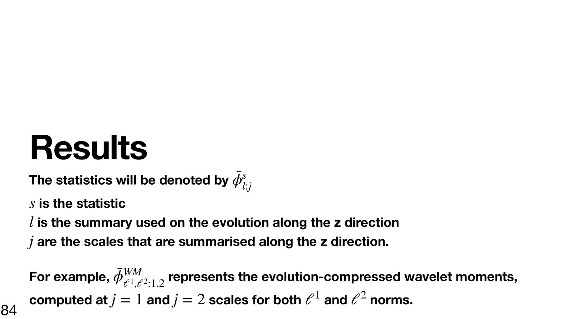
84. Results s The statistics will be denoted by ϕ̄l:j s is the statistic l is the summary used on the evolution along the z direction j are the scales that are summarised along the z direction. WM For example, ϕ̄ℓ 1,ℓ 2:1,2 represents the evolution-compressed wavelet moments, 1 2 84 computed at j = 1 and j = 2 scales for both ℓ and ℓ norms.
85. Results: No Noise 85
86. Results:100 hrs SKA noise 86
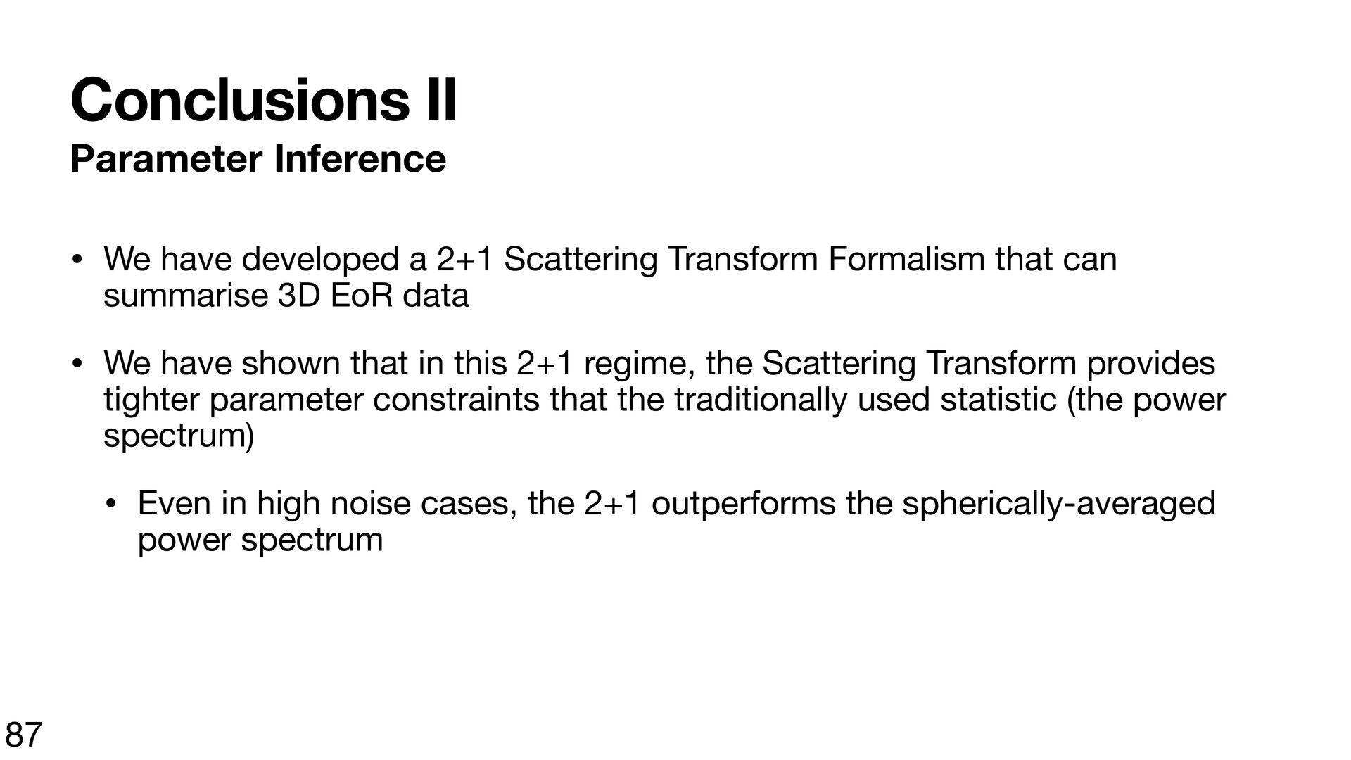
87. Conclusions II Parameter Inference • We have developed a 2+1 Scattering Transform Formalism that can summarise 3D EoR data • We have shown that in this 2+1 regime, the Scattering Transform provides tighter parameter constraints that the traditionally used statistic (the power spectrum) • Even in high noise cases, the 2+1 outperforms the spherically-averaged power spectrum 87
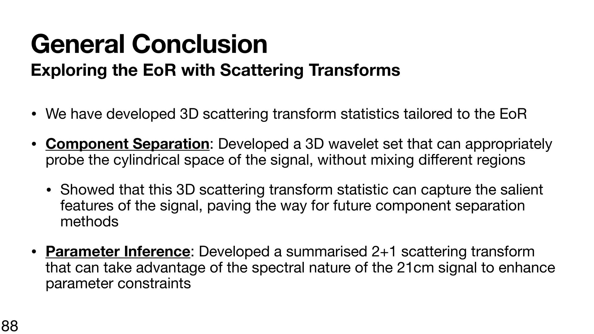
88. General Conclusion Exploring the EoR with Scattering Transforms • We have developed 3D scattering transform statistics tailored to the EoR • Component Separation: Developed a 3D wavelet set that can appropriately probe the cylindrical space of the signal, without mixing di erent regions • Showed that this 3D scattering transform statistic can capture the salient features of the signal, paving the way for future component separation methods • Parameter Inference: Developed a summarised 2+1 scattering transform ff that can take advantage of the spectral nature of the 21cm signal to enhance parameter constraints 88