GT ICR - Gilles Chardon (L2S)

Transcript

1. Localisation et imagerie acoustiques G. Chardon G. Chardon Loc. et imag. acoustiques 1 / 39
2. Sommaire 1 Introduction 2 Localisation de sources Beamforming DAMAS et CMF DAMAS et CLEAN 3 Extensions Localisation hors grille Source corrélées Réseaux asynchrones G. Chardon Loc. et imag. acoustiques 1 / 39
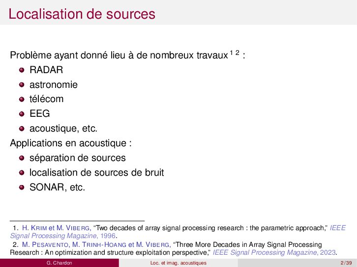
3. Localisation de sources Problème ayant donné lieu à de nombreux travaux 1 2 : RADAR astronomie télécom EEG acoustique, etc. Applications en acoustique : séparation de sources localisation de sources de bruit SONAR, etc. 1. H. KRIM et M. VIBERG, “Two decades of array signal processing research : the parametric approach,” IEEE Signal Processing Magazine, 1996. 2. M. PESAVENTO, M. TRINH-HOANG et M. VIBERG, “Three More Decades in Array Signal Processing Research : An optimization and structure exploitation perspective,” IEEE Signal Processing Magazine, 2023. G. Chardon Loc. et imag. acoustiques 2 / 39
4. Le cas classique : sources en champ lointain g(θ) = eikd sin θn n (1) Méthodes communes avec l’analyse spectrale. G. Chardon Loc. et imag. acoustiques 3 / 39
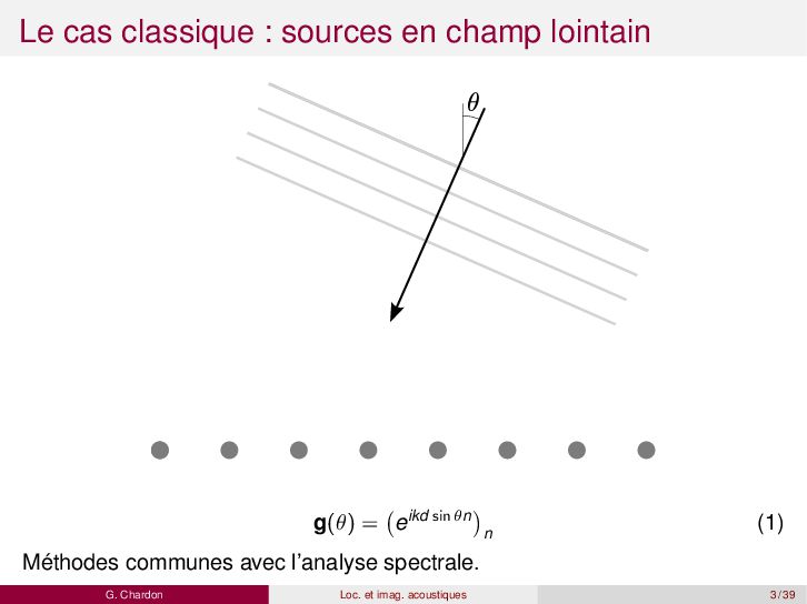
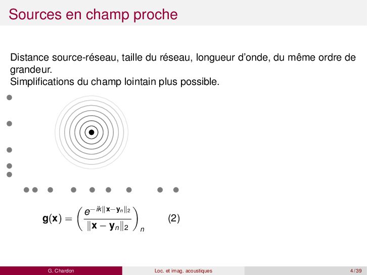
5. Sources en champ proche Distance source-réseau, taille du réseau, longueur d’onde, du même ordre de grandeur. Simplifications du champ lointain plus possible. g(x) = e−ik∥x−yn∥2 ∥x − yn∥2 n (2) G. Chardon Loc. et imag. acoustiques 4 / 39
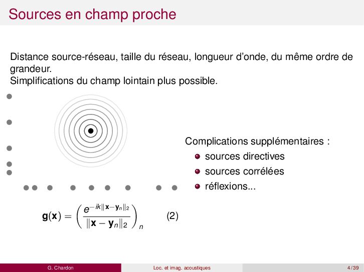
6. Sources en champ proche Distance source-réseau, taille du réseau, longueur d’onde, du même ordre de grandeur. Simplifications du champ lointain plus possible. g(x) = e−ik∥x−yn∥2 ∥x − yn∥2 n (2) Complications supplémentaires : sources directives sources corrélées réflexions... G. Chardon Loc. et imag. acoustiques 4 / 39
7. Modèles de sources Régime fréquentiel Modèle physique : g(x) Modèle conditionnel Paramètres : position x, amplitude A, phase ϕ m ∼ CN(Aeiϕg(x), σ2I). (3) Avantage : simplicité G. Chardon Loc. et imag. acoustiques 5 / 39
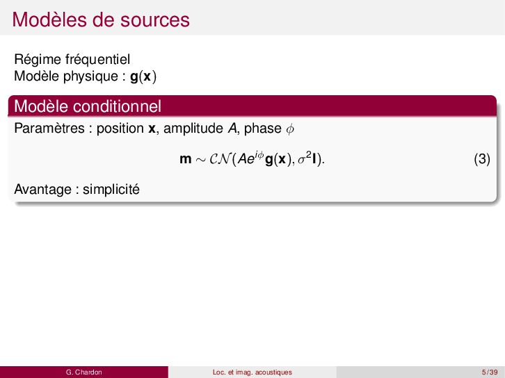
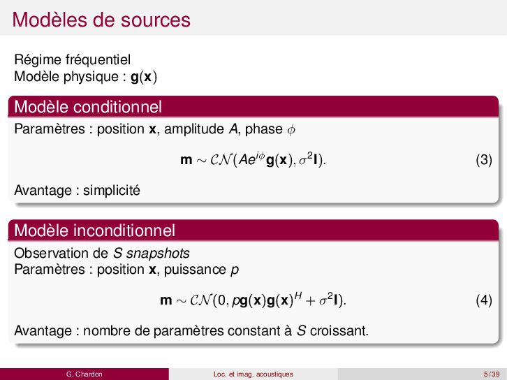
8. Modèles de sources Régime fréquentiel Modèle physique : g(x) Modèle conditionnel Paramètres : position x, amplitude A, phase ϕ m ∼ CN(Aeiϕg(x), σ2I). (3) Avantage : simplicité Modèle inconditionnel Observation de S snapshots Paramètres : position x, puissance p m ∼ CN(0, pg(x)g(x)H + σ2I). (4) Avantage : nombre de paramètres constant à S croissant. G. Chardon Loc. et imag. acoustiques 5 / 39
9. Données expérimentales Mesures à l’Institut d’Alembert (SU) Réseau de 128 microphones MEMS 4 sources, modèle inconditionnel Au L2S : réseau de 32 microphones (enseignement, recherche, médiation) G. Chardon Loc. et imag. acoustiques 6 / 39
10. Sommaire 1 Introduction 2 Localisation de sources Beamforming DAMAS et CMF DAMAS et CLEAN 3 Extensions Localisation hors grille Source corrélées Réseaux asynchrones G. Chardon Loc. et imag. acoustiques 6 / 39
11. Sommaire 1 Introduction 2 Localisation de sources Beamforming DAMAS et CMF DAMAS et CLEAN 3 Extensions Localisation hors grille Source corrélées Réseaux asynchrones G. Chardon Loc. et imag. acoustiques 6 / 39
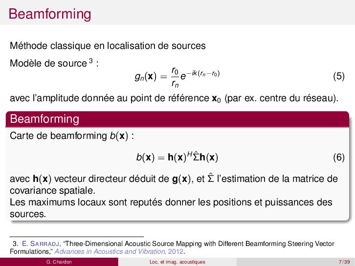
12. Beamforming Méthode classique en localisation de sources Modèle de source 3 : gn(x) = r0 rn e−ik(rn−r0) (5) avec l’amplitude donnée au point de référence x0 (par ex. centre du réseau). Beamforming Carte de beamforming b(x) : b(x) = h(x)H ˆ Σh(x) (6) avec h(x) vecteur directeur déduit de g(x), et ˆ Σ l’estimation de la matrice de covariance spatiale. Les maximums locaux sont reputés donner les positions et puissances des sources. 3. E. SARRADJ, “Three-Dimensional Acoustic Source Mapping with Different Beamforming Steering Vector Formulations,” Advances in Acoustics and Vibration, 2012. G. Chardon Loc. et imag. acoustiques 7 / 39
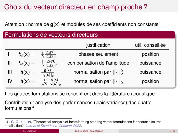
13. Choix du vecteur directeur en champ proche? Attention : norme de g(x) et modules de ses coefficients non constants! Formulations de vecteurs directeurs justification util. conseillée I hn(x) = 1 N gn(x) |gn(x)| phases seulement position II hn(x) = 1 N gn(x) |gn(x)|2 compensation de l’amplitude puissance III h(x) = g(x) ∥g(x)∥2 2 normalisation par ∥ · ∥2 2 puissance IV h(x) = 1 √ N g(x) ∥g(x)∥2 normalisation par ∥ · ∥2 position Les quatres formulations se rencontrent dans la littérature acoustique. Contribution : analyse des performances (biais-variance) des quatre formulations 4. 4. G. CHARDON, “Theoretical analysis of beamforming steering vector formulations for acoustic source localization,” Journal of Sound and Vibration, 2022. G. Chardon Loc. et imag. acoustiques 8 / 39
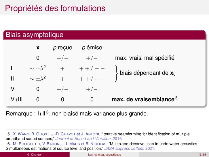
14. Propriétés des formulations Biais asymptotique x p reçue p émise I 0 +/− +/− max. vrais. mal spécifié II ∼ ±λ2 + + + / − − biais dépendant de x0 III ∼ ±λ2 + + + / − − IV 0 +/− +/− IV+III 0 0 0 max. de vraisemblance 5 Remarque : I+II 6, non biaisé mais variance plus grande. 5. X. WANG, B. QUOST, J.-D. CHAZOT et J. ANTONI, “Iterative beamforming for identification of multiple broadband sound sources,” Journal of Sound and Vibration, 2016 6. M. POLICHETTI, V. BARON, J. I. MARS et B. NICOLAS, “Multiplane deconvolution in underwater acoustics : Simultaneous estimations of source level and position,” JASA Express Letters, 2021. G. Chardon Loc. et imag. acoustiques 9 / 39
15. Conclusion Il est nécessaire de combiner deux formulations pour estimer position (IV) et puissance (III) de la source. Interprétation des cartes de beamforming b(x) : III : puissance de la source en supposant qu’elle soit en x IV : vraisemblance de la position x. À compléter par l’estimation du niveau de bruit et comparaison avec la suppression de la diagonale de ˆ Σ. Limitation (connue) du beamforming : résolution de plusieurs sources proches G. Chardon Loc. et imag. acoustiques 10 / 39
16. Sommaire 1 Introduction 2 Localisation de sources Beamforming DAMAS et CMF DAMAS et CLEAN 3 Extensions Localisation hors grille Source corrélées Réseaux asynchrones G. Chardon Loc. et imag. acoustiques 10 / 39
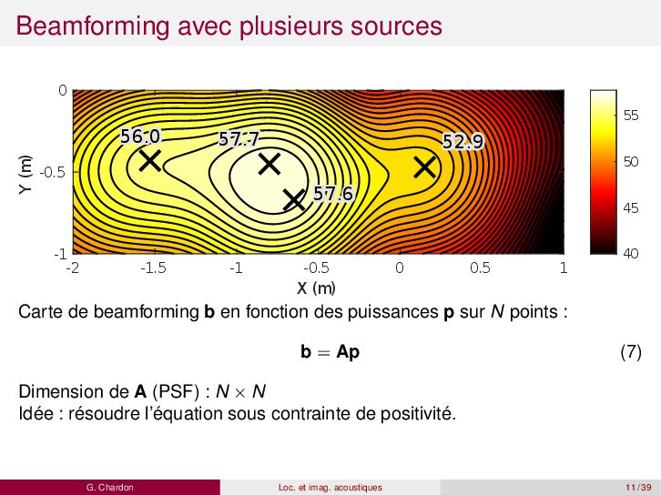
17. Beamforming avec plusieurs sources -2 -1.5 -1 -0.5 0 0.5 1 X (m) -1 -0.5 0 Y (m) 40 45 50 55 56.0 57.6 57.7 52.9 Carte de beamforming b en fonction des puissances p sur N points : b = Ap (7) Dimension de A (PSF) : N × N Idée : résoudre l’équation sous contrainte de positivité. G. Chardon Loc. et imag. acoustiques 11 / 39
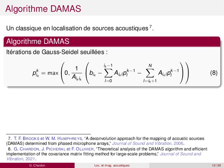
18. Algorithme DAMAS Un classique en localisation de sources acoustiques 7. Algorithme DAMAS Itérations de Gauss-Seidel seuillées : pk ik = max  0, 1 Aik ik  bik − ik −1 l=0 Aik l pk−1 l − N l=ik +1 Aik l pk−1 l     (8) 7. T. F. BROOKS et W. M. HUMPHREYS, “A deconvolution approach for the mapping of acoustic sources (DAMAS) determined from phased microphone arrays,” Journal of Sound and Vibration, 2006. 8. G. CHARDON, J. PICHERAL et F. OLLIVIER, “Theoretical analysis of the DAMAS algorithm and efficient implementation of the covariance matrix fitting method for large-scale problems,” Journal of Sound and Vibration, 2021. G. Chardon Loc. et imag. acoustiques 12 / 39
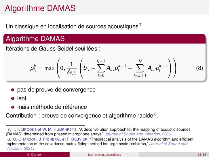
19. Algorithme DAMAS Un classique en localisation de sources acoustiques 7. Algorithme DAMAS Itérations de Gauss-Seidel seuillées : pk ik = max  0, 1 Aik ik  bik − ik −1 l=0 Aik l pk−1 l − N l=ik +1 Aik l pk−1 l     (8) pas de preuve de convergence lent mais méthode de référence Contribution : preuve de convergence et algorithme rapide 8. 7. T. F. BROOKS et W. M. HUMPHREYS, “A deconvolution approach for the mapping of acoustic sources (DAMAS) determined from phased microphone arrays,” Journal of Sound and Vibration, 2006. 8. G. CHARDON, J. PICHERAL et F. OLLIVIER, “Theoretical analysis of the DAMAS algorithm and efficient implementation of the covariance matrix fitting method for large-scale problems,” Journal of Sound and Vibration, 2021. G. Chardon Loc. et imag. acoustiques 12 / 39
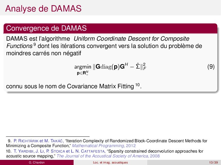
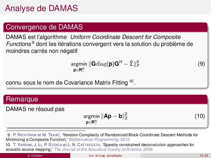
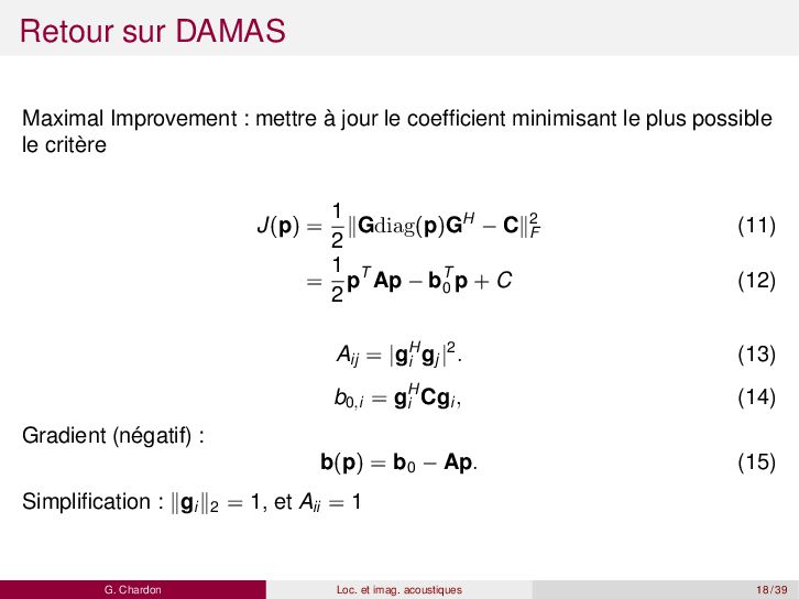
20. Analyse de DAMAS Convergence de DAMAS DAMAS est l’algorithme Uniform Coordinate Descent for Composite Functions 9 dont les itérations convergent vers la solution du problème de moindres carrés non négatif argmin p∈RN + ∥Gdiag(p)GH − ˆ Σ∥2 F (9) connu sous le nom de Covariance Matrix Fitting 10. 9. P. RICHTÁRIK et M. TAKÁ ˇ C, “Iteration Complexity of Randomized Block-Coordinate Descent Methods for Minimizing a Composite Function,” Mathematical Programming, 2012 10. T. YARDIBI, J. LI, P. STOICA et L. N. CATTAFESTA, “Sparsity constrained deconvolution approaches for acoustic source mapping,” The Journal of the Acoustical Society of America, 2008 G. Chardon Loc. et imag. acoustiques 13 / 39
21. Analyse de DAMAS Convergence de DAMAS DAMAS est l’algorithme Uniform Coordinate Descent for Composite Functions 9 dont les itérations convergent vers la solution du problème de moindres carrés non négatif argmin p∈RN + ∥Gdiag(p)GH − ˆ Σ∥2 F (9) connu sous le nom de Covariance Matrix Fitting 10. Remarque DAMAS ne résoud pas argmin p∈RN + ∥Ap − b∥2 2 (10) 9. P. RICHTÁRIK et M. TAKÁ ˇ C, “Iteration Complexity of Randomized Block-Coordinate Descent Methods for Minimizing a Composite Function,” Mathematical Programming, 2012 10. T. YARDIBI, J. LI, P. STOICA et L. N. CATTAFESTA, “Sparsity constrained deconvolution approaches for acoustic source mapping,” The Journal of the Acoustical Society of America, 2008 G. Chardon Loc. et imag. acoustiques 13 / 39
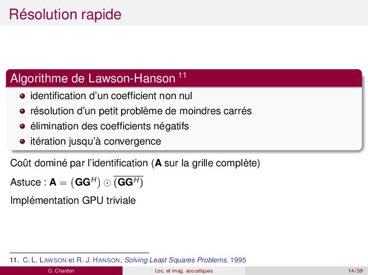
22. Résolution rapide Algorithme de Lawson-Hanson 11 identification d’un coefficient non nul résolution d’un petit problème de moindres carrés élimination des coefficients négatifs itération jusqu’à convergence Coût dominé par l’identification (A sur la grille complète) Astuce : A = GGH ⊙ (GGH) Implémentation GPU triviale 11. C. L. LAWSON et R. J. HANSON, Solving Least Squares Problems. 1995 G. Chardon Loc. et imag. acoustiques 14 / 39
23. Convergence des algorithmes Temps de calcul sur PC portable, N ≈ 104 G. Chardon Loc. et imag. acoustiques 15 / 39
24. Résultats expérimentaux - 2D G. Chardon Loc. et imag. acoustiques 16 / 39
25. Résultats expérimentaux - 3D M = 3, 75.105 A ≈ 1To 7 min. 5 4.5 -1 -0.8 -0.6 -1.5 -0.4 -1 -0.5 0 4 G. Chardon Loc. et imag. acoustiques 17 / 39
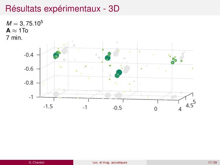
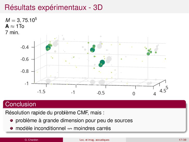
26. Résultats expérimentaux - 3D M = 3, 75.105 A ≈ 1To 7 min. 5 4.5 -1 -0.8 -0.6 -1.5 -0.4 -1 -0.5 0 4 Conclusion Résolution rapide du problème CMF, mais : problème à grande dimension pour peu de sources modèle inconditionnel ↮ moindres carrés G. Chardon Loc. et imag. acoustiques 17 / 39
27. Sommaire 1 Introduction 2 Localisation de sources Beamforming DAMAS et CMF DAMAS et CLEAN 3 Extensions Localisation hors grille Source corrélées Réseaux asynchrones G. Chardon Loc. et imag. acoustiques 17 / 39
28. Retour sur DAMAS Maximal Improvement : mettre à jour le coefficient minimisant le plus possible le critère J(p) = 1 2 ∥Gdiag(p)GH − C∥2 F (11) = 1 2 pT Ap − bT 0 p + C (12) Aij = |gH i gj |2. (13) b0,i = gH i Cgi , (14) Gradient (négatif) : b(p) = b0 − Ap. (15) Simplification : ∥gi ∥2 = 1, et Aii = 1 G. Chardon Loc. et imag. acoustiques 18 / 39
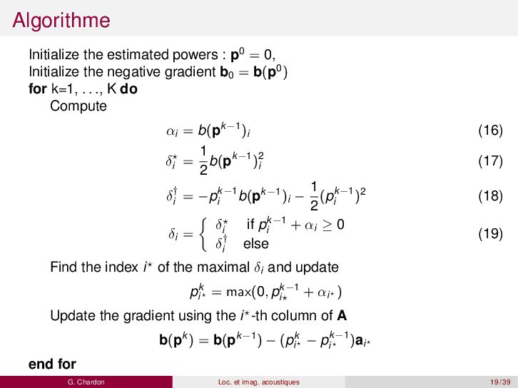
29. Algorithme Initialize the estimated powers : p0 = 0, Initialize the negative gradient b0 = b(p0) for k=1, . . ., K do Compute αi = b(pk−1)i (16) δ⋆ i = 1 2 b(pk−1)2 i (17) δ† i = −pk−1 i b(pk−1)i − 1 2 (pk−1 i )2 (18) δi = δ⋆ i if pk−1 i + αi ≥ 0 δ† i else (19) Find the index i⋆ of the maximal δi and update pk i⋆ = max(0, pk−1 i⋆ + αi⋆ ) Update the gradient using the i⋆-th column of A b(pk ) = b(pk−1) − (pk i⋆ − pk−1 i⋆ )ai⋆ end for G. Chardon Loc. et imag. acoustiques 19 / 39
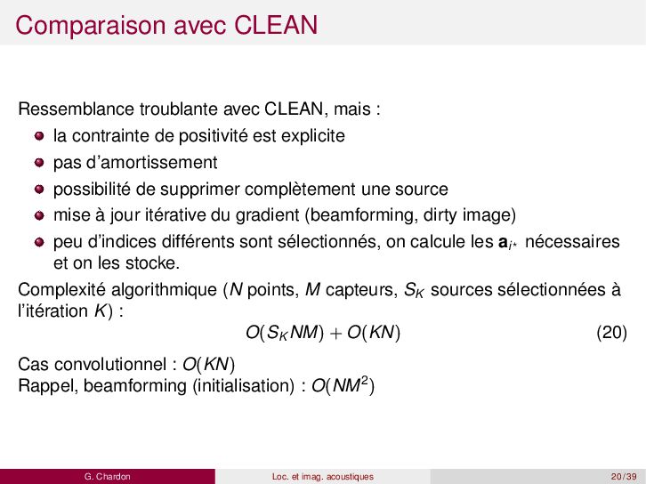
30. Comparaison avec CLEAN Ressemblance troublante avec CLEAN, mais : la contrainte de positivité est explicite pas d’amortissement possibilité de supprimer complètement une source mise à jour itérative du gradient (beamforming, dirty image) peu d’indices différents sont sélectionnés, on calcule les ai⋆ nécessaires et on les stocke. Complexité algorithmique (N points, M capteurs, SK sources sélectionnées à l’itération K) : O(SK NM) + O(KN) (20) Cas convolutionnel : O(KN) Rappel, beamforming (initialisation) : O(NM2) G. Chardon Loc. et imag. acoustiques 20 / 39
31. Résultats numériques Convergence sur un petit problème (N = 7701) 10−1 100 Time (s) 10−6 10−5 10−4 10−3 10−2 10−1 100 101 δ DAMAS-MI cyclic DAMAS random DAMAS roundtrip DAMAS CLEAN-SC ϕ =1 CLEAN-SC ϕ =0.1 LH G. Chardon Loc. et imag. acoustiques 21 / 39
32. Résultats numériques Imagerie en 3D (N = 1121931 points), comparaison DAMAS-MI (gauche, 4.7s) et LH (droite, 17min.) G. Chardon Loc. et imag. acoustiques 22 / 39
33. Sommaire 1 Introduction 2 Localisation de sources Beamforming DAMAS et CMF DAMAS et CLEAN 3 Extensions Localisation hors grille Source corrélées Réseaux asynchrones G. Chardon Loc. et imag. acoustiques 22 / 39
34. Sommaire 1 Introduction 2 Localisation de sources Beamforming DAMAS et CMF DAMAS et CLEAN 3 Extensions Localisation hors grille Source corrélées Réseaux asynchrones G. Chardon Loc. et imag. acoustiques 22 / 39
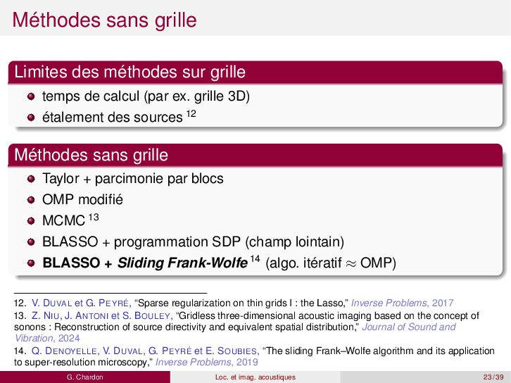
35. Méthodes sans grille Limites des méthodes sur grille temps de calcul (par ex. grille 3D) étalement des sources 12 Méthodes sans grille Taylor + parcimonie par blocs OMP modifié MCMC 13 BLASSO + programmation SDP (champ lointain) BLASSO + Sliding Frank-Wolfe 14 (algo. itératif ≈ OMP) 12. V. DUVAL et G. PEYRÉ, “Sparse regularization on thin grids I : the Lasso,” Inverse Problems, 2017 13. Z. NIU, J. ANTONI et S. BOULEY, “Gridless three-dimensional acoustic imaging based on the concept of sonons : Reconstruction of source directivity and equivalent spatial distribution,” Journal of Sound and Vibration, 2024 14. Q. DENOYELLE, V. DUVAL, G. PEYRÉ et E. SOUBIES, “The sliding Frank–Wolfe algorithm and its application to super-resolution microscopy,” Inverse Problems, 2019 G. Chardon Loc. et imag. acoustiques 23 / 39
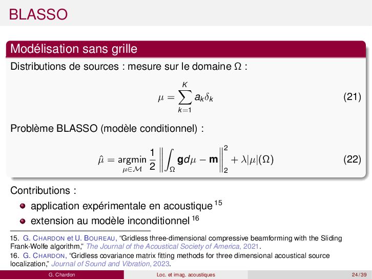
36. BLASSO Modélisation sans grille Distributions de sources : mesure sur le domaine Ω : µ = K k=1 ak δk (21) Problème BLASSO (modèle conditionnel) : ˆ µ = argmin µ∈M 1 2 Ω gdµ − m 2 2 + λ|µ|(Ω) (22) Contributions : application expérimentale en acoustique 15 extension au modèle inconditionnel 16 15. G. CHARDON et U. BOUREAU, “Gridless three-dimensional compressive beamforming with the Sliding Frank-Wolfe algorithm,” The Journal of the Acoustical Society of America, 2021. 16. G. CHARDON, “Gridless covariance matrix fitting methods for three dimensional acoustical source localization,” Journal of Sound and Vibration, 2023. G. Chardon Loc. et imag. acoustiques 24 / 39
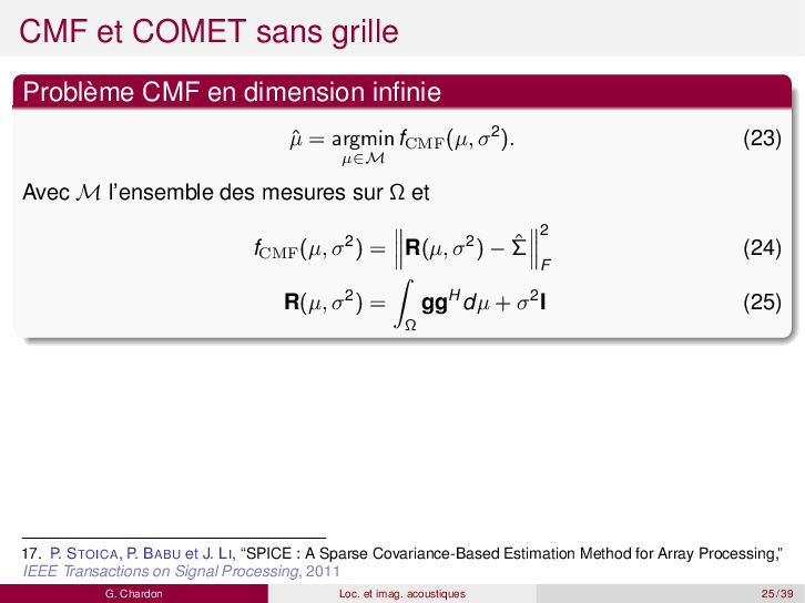
37. CMF et COMET sans grille Problème CMF en dimension infinie ˆ µ = argmin µ∈M fCMF (µ, σ2). (23) Avec M l’ensemble des mesures sur Ω et fCMF (µ, σ2) = R(µ, σ2) − ˆ Σ 2 F (24) R(µ, σ2) = Ω ggHdµ + σ2I (25) 17. P. STOICA, P. BABU et J. LI, “SPICE : A Sparse Covariance-Based Estimation Method for Array Processing,” IEEE Transactions on Signal Processing, 2011 G. Chardon Loc. et imag. acoustiques 25 / 39
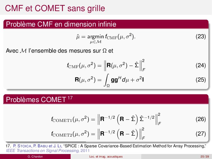
38. CMF et COMET sans grille Problème CMF en dimension infinie ˆ µ = argmin µ∈M fCMF (µ, σ2). (23) Avec M l’ensemble des mesures sur Ω et fCMF (µ, σ2) = R(µ, σ2) − ˆ Σ 2 F (24) R(µ, σ2) = Ω ggHdµ + σ2I (25) Problèmes COMET 17 fCOMET1 (µ, σ2) = R−1/2 R − ˆ Σ ˆ Σ−1/2 2 F (26) fCOMET2 (µ, σ2) = R−1/2 R − ˆ Σ 2 F (27) 17. P. STOICA, P. BABU et J. LI, “SPICE : A Sparse Covariance-Based Estimation Method for Array Processing,” IEEE Transactions on Signal Processing, 2011 G. Chardon Loc. et imag. acoustiques 25 / 39
39. Résultats - simulations MSE pour 4 sources en fonction du SNR étude de la résolution pour deux sources à bas SNR -20 -10 0 10 SNR (dB) 10-4 10-2 100 Position MSE (m 2) COMET2 MUSIC OMP CSC HRCSC 0 0.1 0.2 0.3 0.4 (m) -0.25 -0.2 -0.15 -0.1 -0.05 0 0.05 0.1 0.15 0.2 0.25 Estimated X coordinate (m) COMET2 MUSIC OBF G. Chardon Loc. et imag. acoustiques 26 / 39
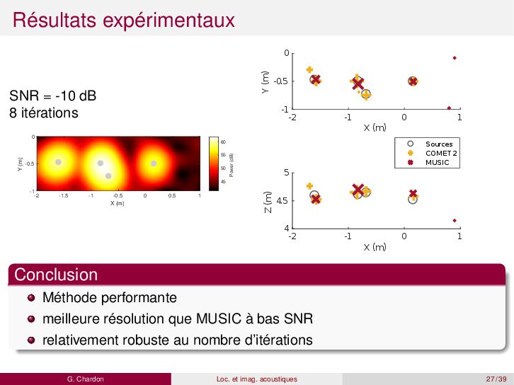
40. Résultats expérimentaux SNR = -10 dB 8 itérations -2 -1.5 -1 -0.5 0 0.5 1 X (m) -1 -0.5 0 Y (m) 45 50 55 60 Power (dB) -2 -1 0 1 X (m) -1 -0.5 0 Y (m) Sources COMET2 MUSIC -2 -1 0 1 X (m) 4 4.5 5 Z (m) Conclusion Méthode performante meilleure résolution que MUSIC à bas SNR relativement robuste au nombre d’itérations G. Chardon Loc. et imag. acoustiques 27 / 39
41. Sommaire 1 Introduction 2 Localisation de sources Beamforming DAMAS et CMF DAMAS et CLEAN 3 Extensions Localisation hors grille Source corrélées Réseaux asynchrones G. Chardon Loc. et imag. acoustiques 27 / 39
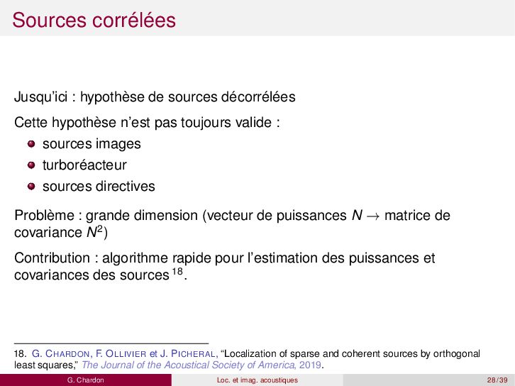
42. Sources corrélées Jusqu’ici : hypothèse de sources décorrélées Cette hypothèse n’est pas toujours valide : sources images turboréacteur sources directives Problème : grande dimension (vecteur de puissances N → matrice de covariance N2) Contribution : algorithme rapide pour l’estimation des puissances et covariances des sources 18. 18. G. CHARDON, F. OLLIVIER et J. PICHERAL, “Localization of sparse and coherent sources by orthogonal least squares,” The Journal of the Acoustical Society of America, 2019. G. Chardon Loc. et imag. acoustiques 28 / 39
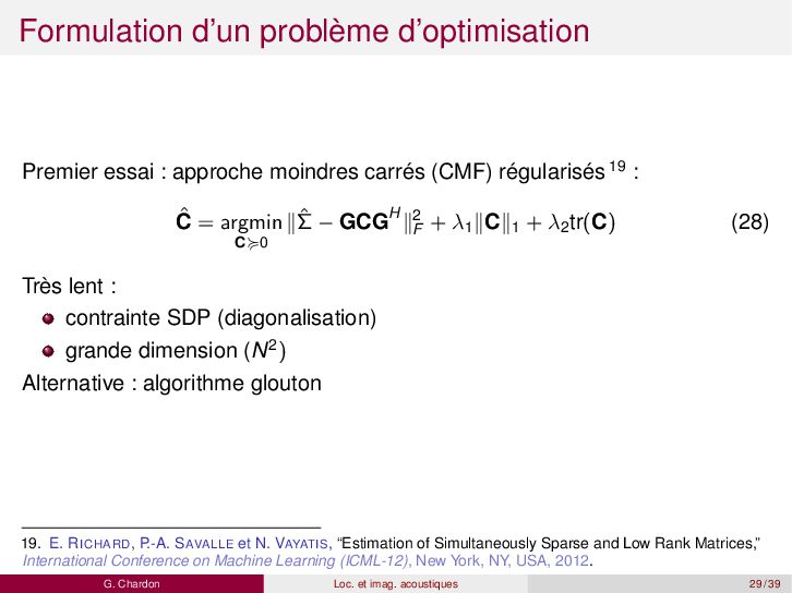
43. Formulation d’un problème d’optimisation Premier essai : approche moindres carrés (CMF) régularisés 19 : ˆ C = argmin C≽0 ∥ˆ Σ − GCGH∥2 F + λ1∥C∥1 + λ2 tr(C) (28) Très lent : contrainte SDP (diagonalisation) grande dimension (N2) Alternative : algorithme glouton 19. E. RICHARD, P.-A. SAVALLE et N. VAYATIS, “Estimation of Simultaneously Sparse and Low Rank Matrices,” International Conference on Machine Learning (ICML-12), New York, NY, USA, 2012. G. Chardon Loc. et imag. acoustiques 29 / 39
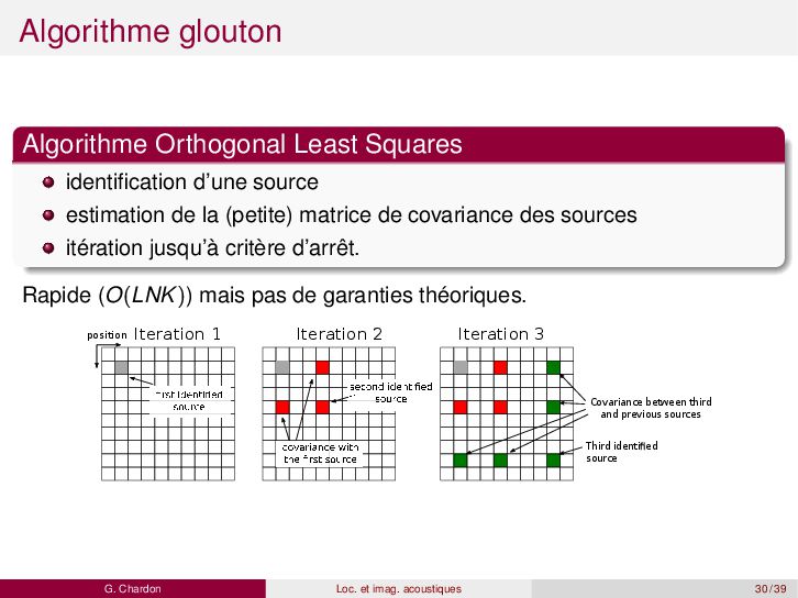
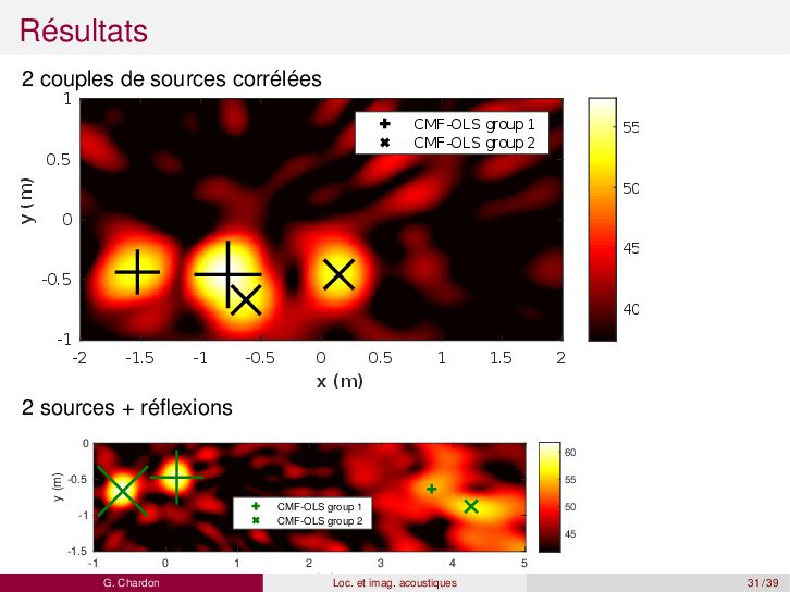
44. Algorithme glouton Algorithme Orthogonal Least Squares identification d’une source estimation de la (petite) matrice de covariance des sources itération jusqu’à critère d’arrêt. Rapide (O(LNK)) mais pas de garanties théoriques. position Third identi ed source Covariance between third and previous sources Iteration 1 Iteration 2 Iteration 3 G. Chardon Loc. et imag. acoustiques 30 / 39
45. Résultats 2 couples de sources corrélées -2 -1.5 -1 -0.5 0 0.5 1 1.5 2 x (m) -1 -0.5 0 0.5 1 y (m) 40 45 50 55 CMF-OLS group 1 CMF-OLS group 2 2 sources + réflexions -1 0 1 2 3 4 5 x (m) -1.5 -1 -0.5 0 y (m) 45 50 55 60 CMF-OLS group 1 CMF-OLS group 2 G. Chardon Loc. et imag. acoustiques 31 / 39
46. Conclusion et perspectives Algorithme OLS preuve de convergence? version sans grille? Hypothèse de décorrélation Pertinente pour des cas d’applications classiques? réflexions sur des surfaces longueur de corrélation en aéroacoustique trajets multiples Comportement des méthodes classiques avec sources corrélées? G. Chardon Loc. et imag. acoustiques 32 / 39
47. Sommaire 1 Introduction 2 Localisation de sources Beamforming DAMAS et CMF DAMAS et CLEAN 3 Extensions Localisation hors grille Source corrélées Réseaux asynchrones G. Chardon Loc. et imag. acoustiques 32 / 39
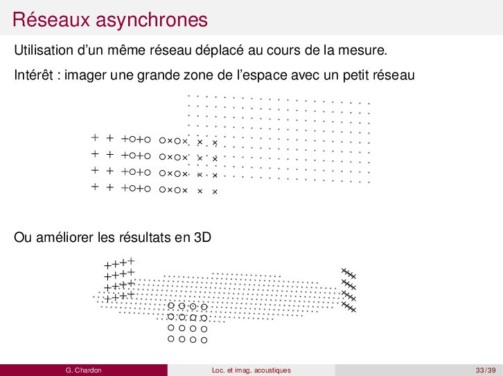
48. Réseaux asynchrones Utilisation d’un même réseau déplacé au cours de la mesure. Intérêt : imager une grande zone de l’espace avec un petit réseau Ou améliorer les résultats en 3D G. Chardon Loc. et imag. acoustiques 33 / 39
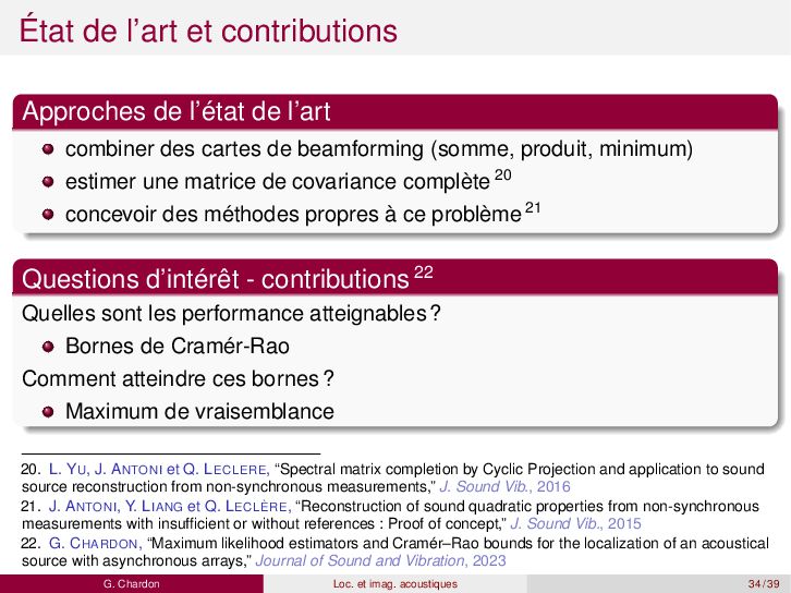
49. État de l’art et contributions Approches de l’état de l’art combiner des cartes de beamforming (somme, produit, minimum) estimer une matrice de covariance complète 20 concevoir des méthodes propres à ce problème 21 Questions d’intérêt - contributions 22 Quelles sont les performance atteignables? Bornes de Cramér-Rao Comment atteindre ces bornes? Maximum de vraisemblance 20. L. YU, J. ANTONI et Q. LECLERE, “Spectral matrix completion by Cyclic Projection and application to sound source reconstruction from non-synchronous measurements,” J. Sound Vib., 2016 21. J. ANTONI, Y. LIANG et Q. LECLÈRE, “Reconstruction of sound quadratic properties from non-synchronous measurements with insufficient or without references : Proof of concept,” J. Sound Vib., 2015 22. G. CHARDON, “Maximum likelihood estimators and Cramér–Rao bounds for the localization of an acoustical source with asynchronous arrays,” Journal of Sound and Vibration, 2023 G. Chardon Loc. et imag. acoustiques 34 / 39
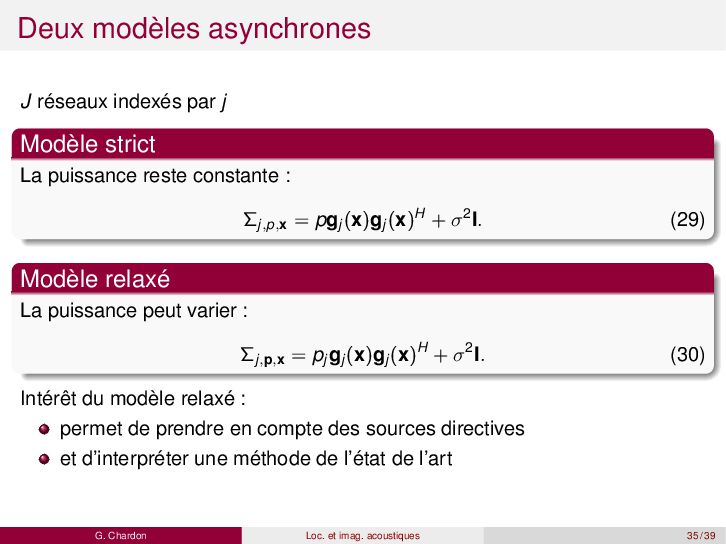
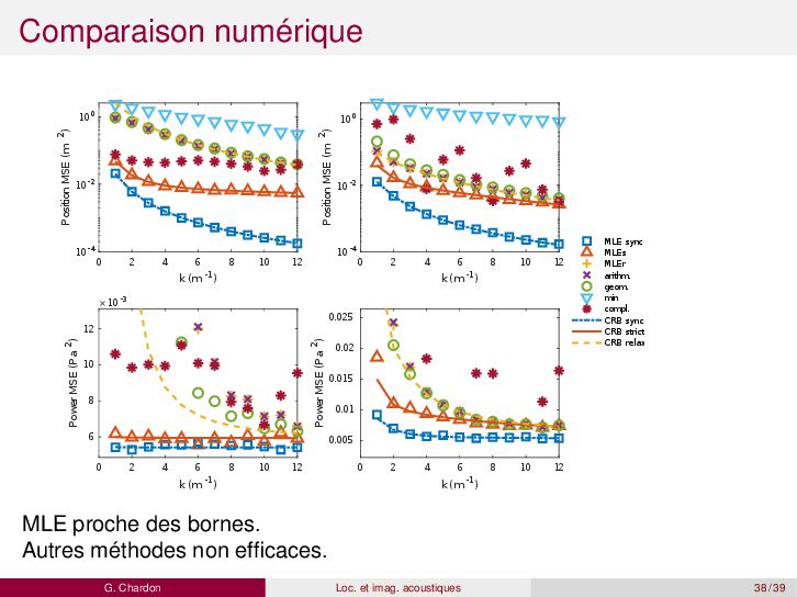
50. Deux modèles asynchrones J réseaux indexés par j Modèle strict La puissance reste constante : Σj,p,x = pgj (x)gj (x)H + σ2I. (29) Modèle relaxé La puissance peut varier : Σj,p,x = pj gj (x)gj (x)H + σ2I. (30) Intérêt du modèle relaxé : permet de prendre en compte des sources directives et d’interpréter une méthode de l’état de l’art G. Chardon Loc. et imag. acoustiques 35 / 39
51. Bornes de Cramér-Rao Position Puissance G. Chardon Loc. et imag. acoustiques 36 / 39
52. Estimation par maximum de vraisemblance Modèle relaxé Moyenne arithmétique des critères de chaque réseau (beamforming IV) Modèle strict (ˆ x, ˆ p) = argmin x∈Ω,p∈R+ J j=1 Sj − pgj (x)H ˆ Σj gj (x) σ2(σ2 + p∥gj (x)∥2) + log(σ2 + p∥gj (x)∥2) (31) Pas d’estimation en deux étapes (position puis puissance). G. Chardon Loc. et imag. acoustiques 37 / 39
53. Comparaison numérique 0 2 4 6 8 10 12 k (m -1) 10-4 10-2 100 Position MSE (m 2) 0 2 4 6 8 10 12 k (m -1) 6 8 10 12 Power MSE (Pa 2) 10-3 0 2 4 6 8 10 12 k (m -1) 10-4 10-2 100 Position MSE (m 2) MLE sync MLEs MLEr arithm. geom. min compl. CRB sync CRB strict CRB relax 0 2 4 6 8 10 12 k (m -1) 0.005 0.01 0.015 0.02 0.025 Power MSE (Pa 2) MLE proche des bornes. Autres méthodes non efficaces. G. Chardon Loc. et imag. acoustiques 38 / 39
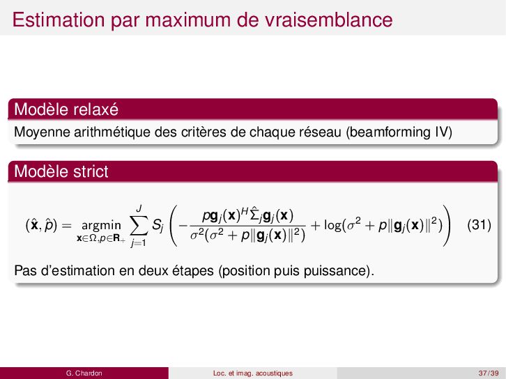
54. Conclusions Problème à une source Il est illusoire d’espérer les mêmes performances qu’un réseau asynchrone. MLE ⇒ estimation jointe de x et p moyenne des beamforming = modèle relaxé moins performant complétion de matrice en échec Perspectives performances des méthodes de complétion quand elles fonctionnent intérêt des microphones de référence extension à plusieurs sources G. Chardon Loc. et imag. acoustiques 39 / 39