GT ICR - Lucien Bacharach (SATIE)

Transcript

1. Optimisation de la configuration de réseaux d’antennes : critères basés sur des bornes d’erreur d’estimation GT "Imagerie computationnelle pour la radioastronomie" @ Saclay Lucien Bacharach, en collaboration avec Jianhua Wang, Iyed Dammak, Pascal Larzabal (SATIE), Mohammed Nabil El Korso (L2S) et Joana Frontera Pons (ONERA) 17 novembre 2025 L. Bacharach – SATIE GT ICR @ Saclay 17/11/2025 1 / 41
2. Outline 1 Contexte Interféométrie radio Projet ANR PerDRIX : partenaires et problèmes traités 2 Bornes d’erreur d’estimation pour le placement des antennes Bornes inférieures de l’erreur quadratique moyenne (du MSE) classiques Exemple : estimation de la fréquence d’un signal sinusoïdal (complexe) Bornes d’erreur pour le placement d’antennes Vers des bornes plus pertinentes pour le placement des antennes ? 3 Conclusions, perspectives L. Bacharach – SATIE GT ICR @ Saclay 17/11/2025 2 / 41
3. Outline 1 Contexte Interféométrie radio Projet ANR PerDRIX : partenaires et problèmes traités 2 Bornes d’erreur d’estimation pour le placement des antennes Bornes inférieures de l’erreur quadratique moyenne (du MSE) classiques Exemple : estimation de la fréquence d’un signal sinusoïdal (complexe) Bornes d’erreur pour le placement d’antennes Vers des bornes plus pertinentes pour le placement des antennes ? 3 Conclusions, perspectives L. Bacharach – SATIE GT ICR @ Saclay 17/11/2025 2 / 41
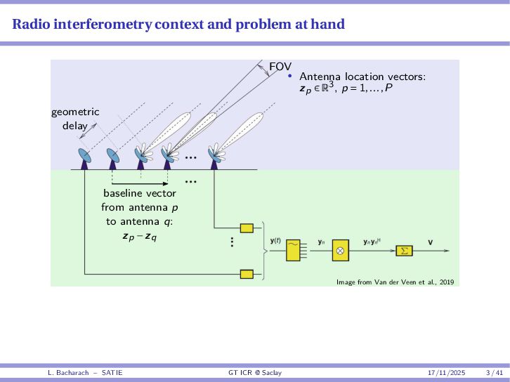
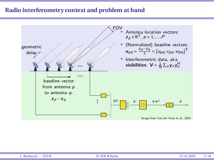
4. Radio interferometry context and problem at hand • Antenna location vectors: zp ∈ R3, p = 1,...,P geometric delay FOV baseline vector from antenna p to antenna q: zp −zq Image from Van der Veen et al., 2019 L. Bacharach – SATIE GT ICR @ Saclay 17/11/2025 3 / 41
5. Radio interferometry context and problem at hand • Antenna location vectors: zp ∈ R3, p = 1,...,P • (Normalized) baseline vectors: upq = zp−zq λ = [upq,vpq,wpq]T geometric delay FOV baseline vector from antenna p to antenna q: zp −zq Image from Van der Veen et al., 2019 L. Bacharach – SATIE GT ICR @ Saclay 17/11/2025 3 / 41
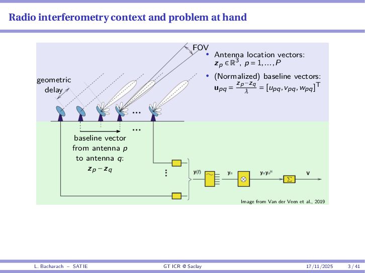
6. Radio interferometry context and problem at hand • Antenna location vectors: zp ∈ R3, p = 1,...,P • (Normalized) baseline vectors: upq = zp−zq λ = [upq,vpq,wpq]T • Interferometric data, aka visibilities: V = 1 N n yn yH n geometric delay FOV baseline vector from antenna p to antenna q: zp −zq Image from Van der Veen et al., 2019 L. Bacharach – SATIE GT ICR @ Saclay 17/11/2025 3 / 41
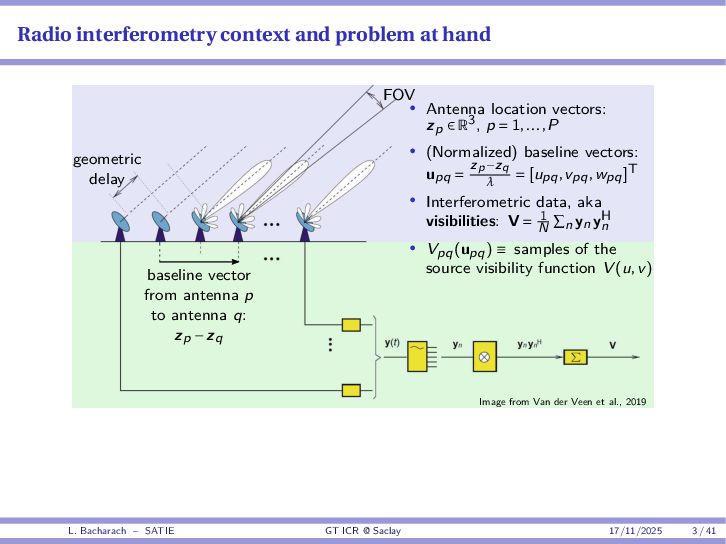
7. Radio interferometry context and problem at hand • Antenna location vectors: zp ∈ R3, p = 1,...,P • (Normalized) baseline vectors: upq = zp−zq λ = [upq,vpq,wpq]T • Interferometric data, aka visibilities: V = 1 N n yn yH n • Vpq(upq) ≡ samples of the source visibility function V (u,v) geometric delay FOV baseline vector from antenna p to antenna q: zp −zq Image from Van der Veen et al., 2019 L. Bacharach – SATIE GT ICR @ Saclay 17/11/2025 3 / 41
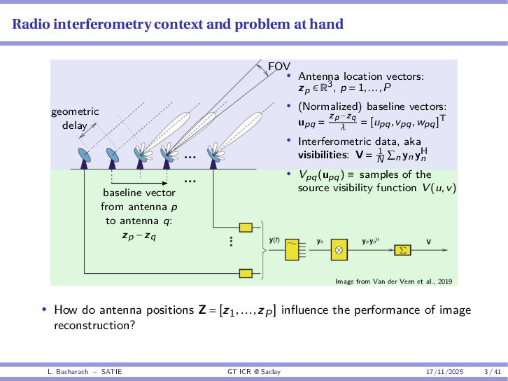
8. Radio interferometry context and problem at hand • Antenna location vectors: zp ∈ R3, p = 1,...,P • (Normalized) baseline vectors: upq = zp−zq λ = [upq,vpq,wpq]T • Interferometric data, aka visibilities: V = 1 N n yn yH n • Vpq(upq) ≡ samples of the source visibility function V (u,v) geometric delay FOV baseline vector from antenna p to antenna q: zp −zq Image from Van der Veen et al., 2019 • How do antenna positions Z = [z1,...,zP] influence the performance of image reconstruction? L. Bacharach – SATIE GT ICR @ Saclay 17/11/2025 3 / 41
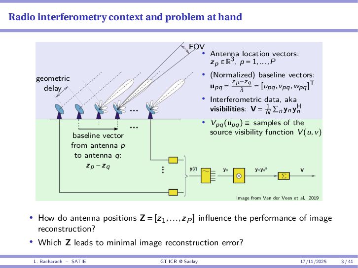
9. Radio interferometry context and problem at hand • Antenna location vectors: zp ∈ R3, p = 1,...,P • (Normalized) baseline vectors: upq = zp−zq λ = [upq,vpq,wpq]T • Interferometric data, aka visibilities: V = 1 N n yn yH n • Vpq(upq) ≡ samples of the source visibility function V (u,v) geometric delay FOV baseline vector from antenna p to antenna q: zp −zq Image from Van der Veen et al., 2019 • How do antenna positions Z = [z1,...,zP] influence the performance of image reconstruction? • Which Z leads to minimal image reconstruction error? L. Bacharach – SATIE GT ICR @ Saclay 17/11/2025 3 / 41
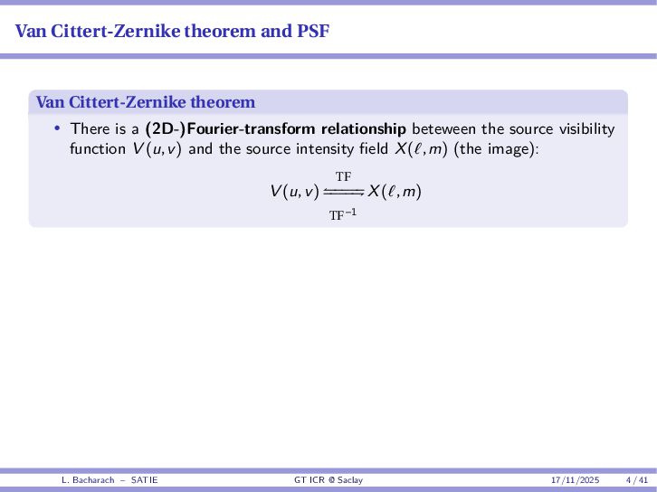
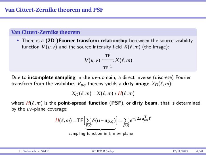
10. Van Cittert-Zernike theorem and PSF Van Cittert-Zernike theorem • There is a (2D-)Fourier-transform relationship beteween the source visibility function V (u,v) and the source intensity field X(ℓ,m) (the image): V (u,v) TF − − − − − − − − TF−1 X(ℓ,m) L. Bacharach – SATIE GT ICR @ Saclay 17/11/2025 4 / 41
11. Van Cittert-Zernike theorem and PSF Van Cittert-Zernike theorem • There is a (2D-)Fourier-transform relationship beteween the source visibility function V (u,v) and the source intensity field X(ℓ,m) (the image): V (u,v) TF − − − − − − − − TF−1 X(ℓ,m) Due to incomplete sampling in the uv-domain, a direct inverse (discrete) Fourier transform from the visibilities Vpq thereby yields a dirty image XD(ℓ,m): XD(ℓ,m) = X(ℓ,m)∗H(ℓ,m) where H(ℓ,m) is the point-spread function (PSF), or dirty beam, that is determined by the uv-plane coverage: H(ℓ,m) = TF p,q δ(u−up,q) sampling function in the uv-plane = p,q e−j2πuT pqℓ L. Bacharach – SATIE GT ICR @ Saclay 17/11/2025 4 / 41
12. Principles of radio interferometry: uv-plane, PSF and dirty image Illustrations generated using APSYNSIM application, I. Martí Vidal. L. Bacharach – SATIE GT ICR @ Saclay 17/11/2025 5 / 41
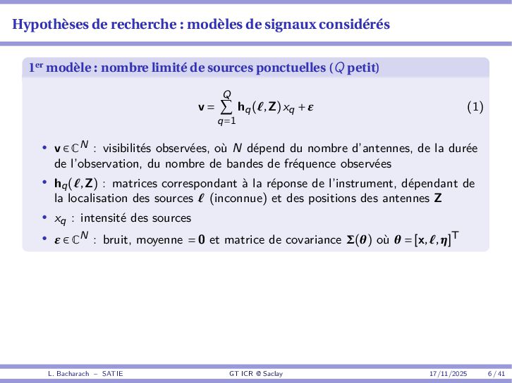
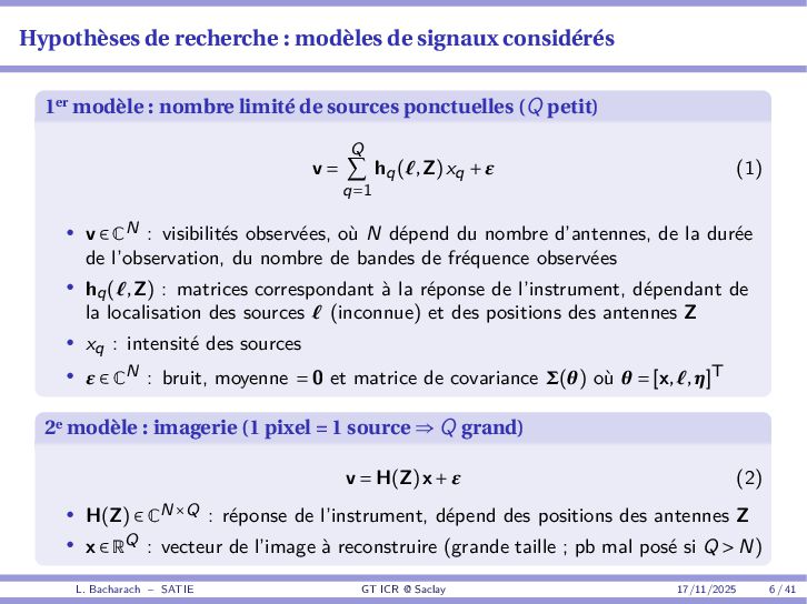
13. Hypothèses de recherche : modèles de signaux considérés 1er modèle : nombre limité de sources ponctuelles (Q petit) v = Q q=1 hq(ℓ,Z)xq +ε (1) • v ∈ CN : visibilités observées, où N dépend du nombre d’antennes, de la durée de l’observation, du nombre de bandes de fréquence observées • hq(ℓ,Z) : matrices correspondant à la réponse de l’instrument, dépendant de la localisation des sources ℓ (inconnue) et des positions des antennes Z • xq : intensité des sources • ε ∈ CN : bruit, moyenne = 0 et matrice de covariance Σ(θ) où θ = [x,ℓ,η]T L. Bacharach – SATIE GT ICR @ Saclay 17/11/2025 6 / 41
14. Hypothèses de recherche : modèles de signaux considérés 1er modèle : nombre limité de sources ponctuelles (Q petit) v = Q q=1 hq(ℓ,Z)xq +ε (1) • v ∈ CN : visibilités observées, où N dépend du nombre d’antennes, de la durée de l’observation, du nombre de bandes de fréquence observées • hq(ℓ,Z) : matrices correspondant à la réponse de l’instrument, dépendant de la localisation des sources ℓ (inconnue) et des positions des antennes Z • xq : intensité des sources • ε ∈ CN : bruit, moyenne = 0 et matrice de covariance Σ(θ) où θ = [x,ℓ,η]T 2e modèle : imagerie (1 pixel = 1 source ⇒ Q grand) v = H(Z)x+ε (2) • H(Z) ∈ CN×Q : réponse de l’instrument, dépend des positions des antennes Z • x ∈ RQ : vecteur de l’image à reconstruire (grande taille ; pb mal posé si Q > N) L. Bacharach – SATIE GT ICR @ Saclay 17/11/2025 6 / 41
15. Outline 1 Contexte Interféométrie radio Projet ANR PerDRIX : partenaires et problèmes traités 2 Bornes d’erreur d’estimation pour le placement des antennes Bornes inférieures de l’erreur quadratique moyenne (du MSE) classiques Exemple : estimation de la fréquence d’un signal sinusoïdal (complexe) Bornes d’erreur pour le placement d’antennes Vers des bornes plus pertinentes pour le placement des antennes ? 3 Conclusions, perspectives L. Bacharach – SATIE GT ICR @ Saclay 17/11/2025 7 / 41
16. Projet ANR JCJC “PerDRIX” : Partenaires • Lucien Bacharach (EC) • Jianhua Wang (PhD student) • Isabelle Vin (EC) • Pascal Larzabal (EC) Signal and array processing Calibration and imaging methods • Julien Girard (EC) Radio astronomy and interferometer design • Mohammed Nabil El Korso (EC) • Gilles Chardon (EC) Inverse problems, sensor placement L. Bacharach – SATIE GT ICR @ Saclay 17/11/2025 8 / 41
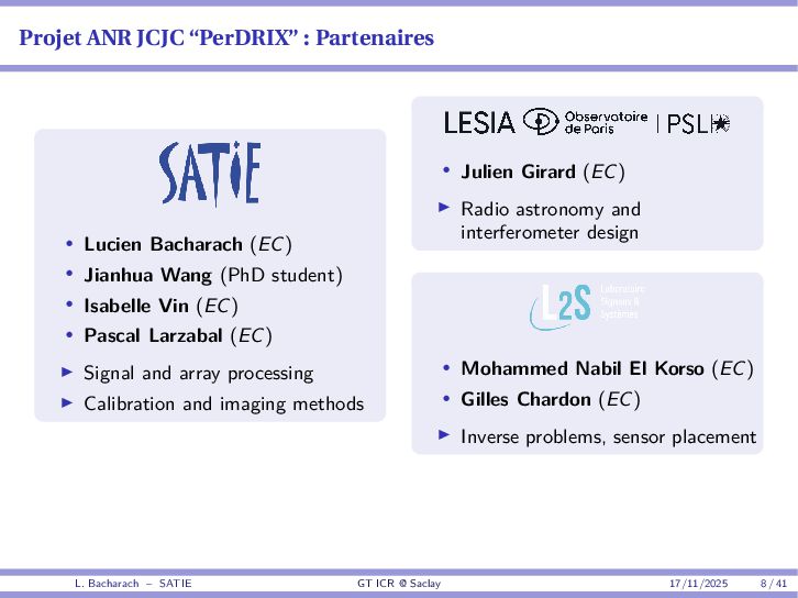
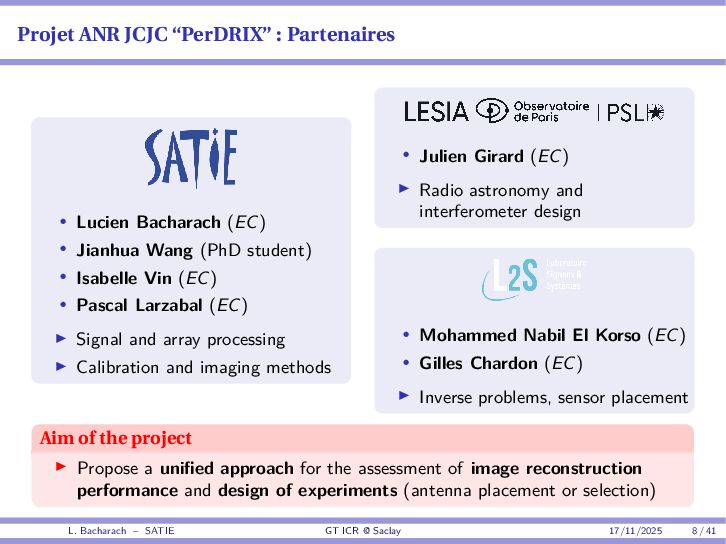
17. Projet ANR JCJC “PerDRIX” : Partenaires • Lucien Bacharach (EC) • Jianhua Wang (PhD student) • Isabelle Vin (EC) • Pascal Larzabal (EC) Signal and array processing Calibration and imaging methods • Julien Girard (EC) Radio astronomy and interferometer design • Mohammed Nabil El Korso (EC) • Gilles Chardon (EC) Inverse problems, sensor placement Aim of the project Propose a unified approach for the assessment of image reconstruction performance and design of experiments (antenna placement or selection) L. Bacharach – SATIE GT ICR @ Saclay 17/11/2025 8 / 41
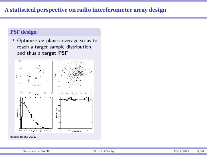
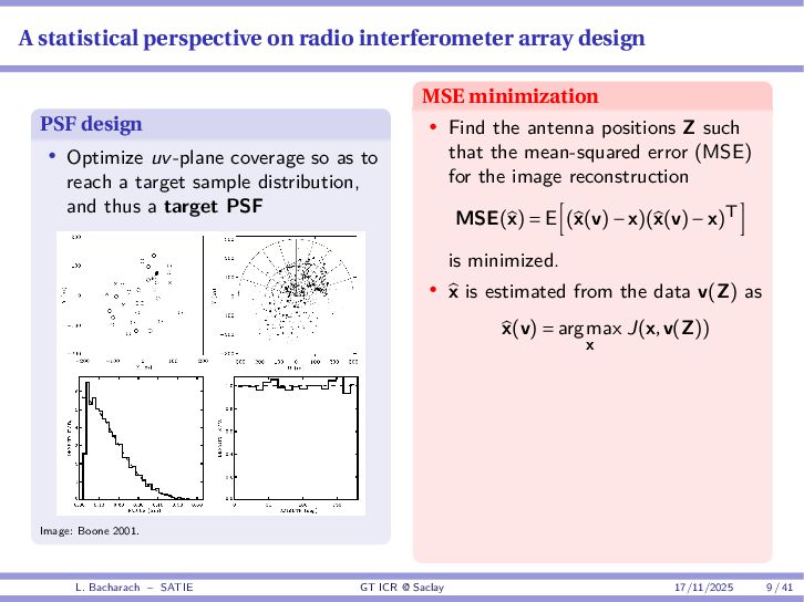
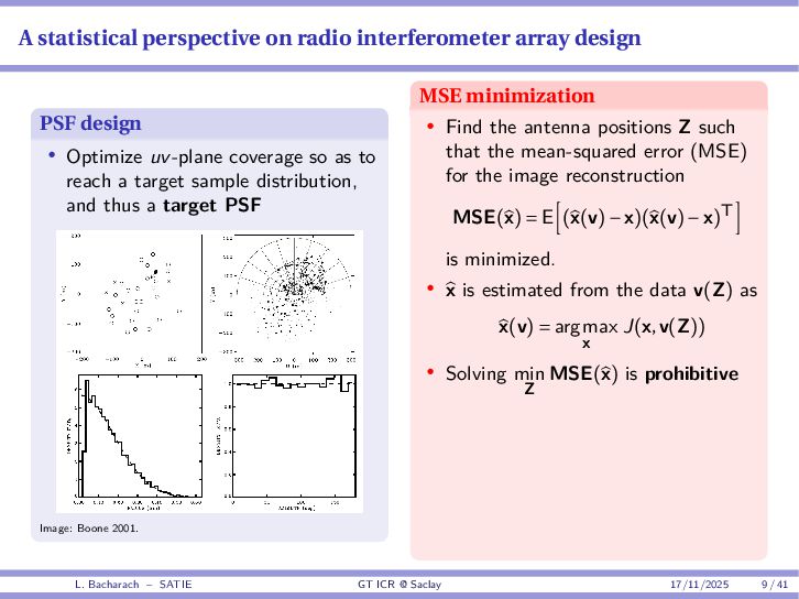
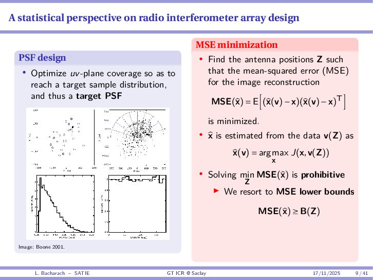
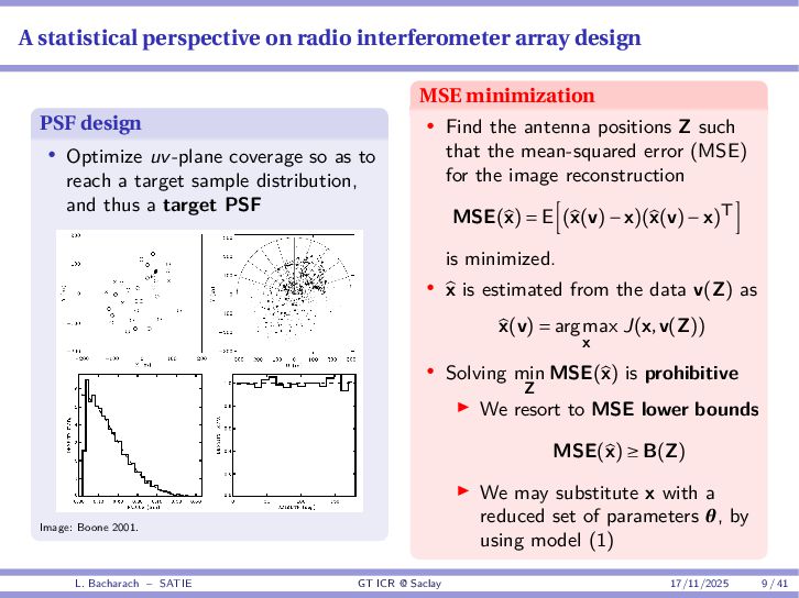
18. A statistical perspective on radio interferometer array design PSF design • Optimize uv-plane coverage so as to reach a target sample distribution, and thus a target PSF Image: Boone 2001. L. Bacharach – SATIE GT ICR @ Saclay 17/11/2025 9 / 41
19. A statistical perspective on radio interferometer array design PSF design • Optimize uv-plane coverage so as to reach a target sample distribution, and thus a target PSF Image: Boone 2001. MSE minimization • Find the antenna positions Z such that the mean-squared error (MSE) for the image reconstruction MSE(x) = E (x(v)−x)(x(v)−x)T is minimized. • x is estimated from the data v(Z) as x(v) = argmax x J(x,v(Z)) L. Bacharach – SATIE GT ICR @ Saclay 17/11/2025 9 / 41
20. A statistical perspective on radio interferometer array design PSF design • Optimize uv-plane coverage so as to reach a target sample distribution, and thus a target PSF Image: Boone 2001. MSE minimization • Find the antenna positions Z such that the mean-squared error (MSE) for the image reconstruction MSE(x) = E (x(v)−x)(x(v)−x)T is minimized. • x is estimated from the data v(Z) as x(v) = argmax x J(x,v(Z)) • Solving min Z MSE(x) is prohibitive L. Bacharach – SATIE GT ICR @ Saclay 17/11/2025 9 / 41
21. A statistical perspective on radio interferometer array design PSF design • Optimize uv-plane coverage so as to reach a target sample distribution, and thus a target PSF Image: Boone 2001. MSE minimization • Find the antenna positions Z such that the mean-squared error (MSE) for the image reconstruction MSE(x) = E (x(v)−x)(x(v)−x)T is minimized. • x is estimated from the data v(Z) as x(v) = argmax x J(x,v(Z)) • Solving min Z MSE(x) is prohibitive We resort to MSE lower bounds MSE(x) ≥ B(Z) L. Bacharach – SATIE GT ICR @ Saclay 17/11/2025 9 / 41
22. A statistical perspective on radio interferometer array design PSF design • Optimize uv-plane coverage so as to reach a target sample distribution, and thus a target PSF Image: Boone 2001. MSE minimization • Find the antenna positions Z such that the mean-squared error (MSE) for the image reconstruction MSE(x) = E (x(v)−x)(x(v)−x)T is minimized. • x is estimated from the data v(Z) as x(v) = argmax x J(x,v(Z)) • Solving min Z MSE(x) is prohibitive We resort to MSE lower bounds MSE(x) ≥ B(Z) We may substitute x with a reduced set of parameters θ, by using model (1) L. Bacharach – SATIE GT ICR @ Saclay 17/11/2025 9 / 41
23. PerDRIX project: work-packages and objectives WP1: Imaging accuracy limits of interferometric arrays Aim: Derive insightful MSE bounds to characterize imaging capabilities of radio interferometers L. Bacharach – SATIE GT ICR @ Saclay 17/11/2025 10 / 41
24. PerDRIX project: work-packages and objectives WP1: Imaging accuracy limits of interferometric arrays Aim: Derive insightful MSE bounds to characterize imaging capabilities of radio interferometers WP2: Optimization of interferometric array lay-out Aim: Develop scalable optimization schemes for optimal antenna placement L. Bacharach – SATIE GT ICR @ Saclay 17/11/2025 10 / 41
25. PerDRIX project: work-packages and objectives WP1: Imaging accuracy limits of interferometric arrays Aim: Derive insightful MSE bounds to characterize imaging capabilities of radio interferometers WP2: Optimization of interferometric array lay-out Aim: Develop scalable optimization schemes for optimal antenna placement WP3: Design of radio interferometers and observations Aim: Assess proposed methodology in practical use cases L. Bacharach – SATIE GT ICR @ Saclay 17/11/2025 10 / 41
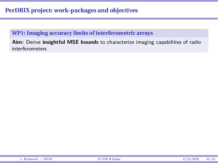
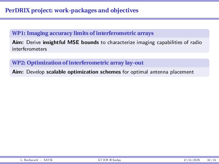
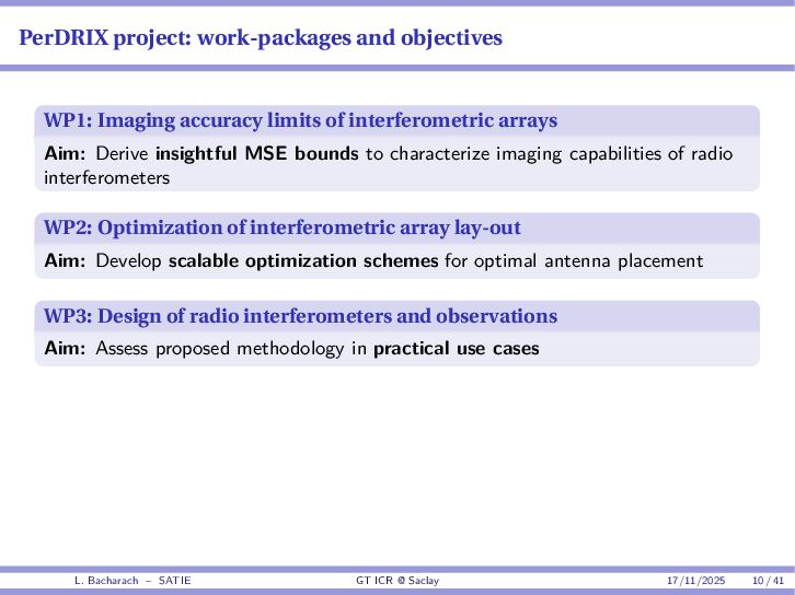
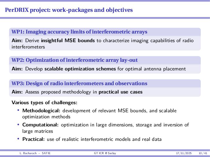
26. PerDRIX project: work-packages and objectives WP1: Imaging accuracy limits of interferometric arrays Aim: Derive insightful MSE bounds to characterize imaging capabilities of radio interferometers WP2: Optimization of interferometric array lay-out Aim: Develop scalable optimization schemes for optimal antenna placement WP3: Design of radio interferometers and observations Aim: Assess proposed methodology in practical use cases Various types of challenges: • Methodological: development of relevant MSE bounds, and scalable optimization methods • Computational: optimization in large dimensions, storage and inversion of large matrices • Practical: use of realistic interferometric models and real data L. Bacharach – SATIE GT ICR @ Saclay 17/11/2025 10 / 41
27. Outline 1 Contexte Interféométrie radio Projet ANR PerDRIX : partenaires et problèmes traités 2 Bornes d’erreur d’estimation pour le placement des antennes Bornes inférieures de l’erreur quadratique moyenne (du MSE) classiques Exemple : estimation de la fréquence d’un signal sinusoïdal (complexe) Bornes d’erreur pour le placement d’antennes Vers des bornes plus pertinentes pour le placement des antennes ? 3 Conclusions, perspectives L. Bacharach – SATIE GT ICR @ Saclay 17/11/2025 11 / 41
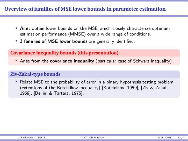
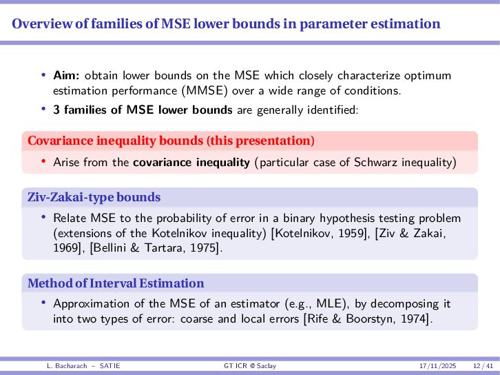
28. Overview of families of MSE lower bounds in parameter estimation • Aim: obtain lower bounds on the MSE which closely characterize optimum estimation performance (MMSE) over a wide range of conditions. • 3 families of MSE lower bounds are generally identified: L. Bacharach – SATIE GT ICR @ Saclay 17/11/2025 12 / 41
29. Overview of families of MSE lower bounds in parameter estimation • Aim: obtain lower bounds on the MSE which closely characterize optimum estimation performance (MMSE) over a wide range of conditions. • 3 families of MSE lower bounds are generally identified: Covariance inequality bounds (this presentation) • Arise from the covariance inequality (particular case of Schwarz inequality) L. Bacharach – SATIE GT ICR @ Saclay 17/11/2025 12 / 41
30. Overview of families of MSE lower bounds in parameter estimation • Aim: obtain lower bounds on the MSE which closely characterize optimum estimation performance (MMSE) over a wide range of conditions. • 3 families of MSE lower bounds are generally identified: Covariance inequality bounds (this presentation) • Arise from the covariance inequality (particular case of Schwarz inequality) Ziv-Zakai-type bounds • Relate MSE to the probability of error in a binary hypothesis testing problem (extensions of the Kotelnikov inequality) [Kotelnikov, 1959], [Ziv & Zakai, 1969], [Bellini & Tartara, 1975]. L. Bacharach – SATIE GT ICR @ Saclay 17/11/2025 12 / 41
31. Overview of families of MSE lower bounds in parameter estimation • Aim: obtain lower bounds on the MSE which closely characterize optimum estimation performance (MMSE) over a wide range of conditions. • 3 families of MSE lower bounds are generally identified: Covariance inequality bounds (this presentation) • Arise from the covariance inequality (particular case of Schwarz inequality) Ziv-Zakai-type bounds • Relate MSE to the probability of error in a binary hypothesis testing problem (extensions of the Kotelnikov inequality) [Kotelnikov, 1959], [Ziv & Zakai, 1969], [Bellini & Tartara, 1975]. Method of Interval Estimation • Approximation of the MSE of an estimator (e.g., MLE), by decomposing it into two types of error: coarse and local errors [Rife & Boorstyn, 1974]. L. Bacharach – SATIE GT ICR @ Saclay 17/11/2025 12 / 41
32. Covariance inequality • The most standard form of the covariance inequality directly results from Schwarz inequality: for any estimator θ and any function v(y,θ) that verifies E[v2(y,θ)] < ∞, or, defining ϵ(y,θ) = θ(y)−θ, Var(θ) ≥ (cov(θ,v))2 Var(v) MSE(θ) ≥ E[ϵ(y,θ)v(y,θ)] 2 E[v2(y,θ)] L. Bacharach – SATIE GT ICR @ Saclay 17/11/2025 13 / 41
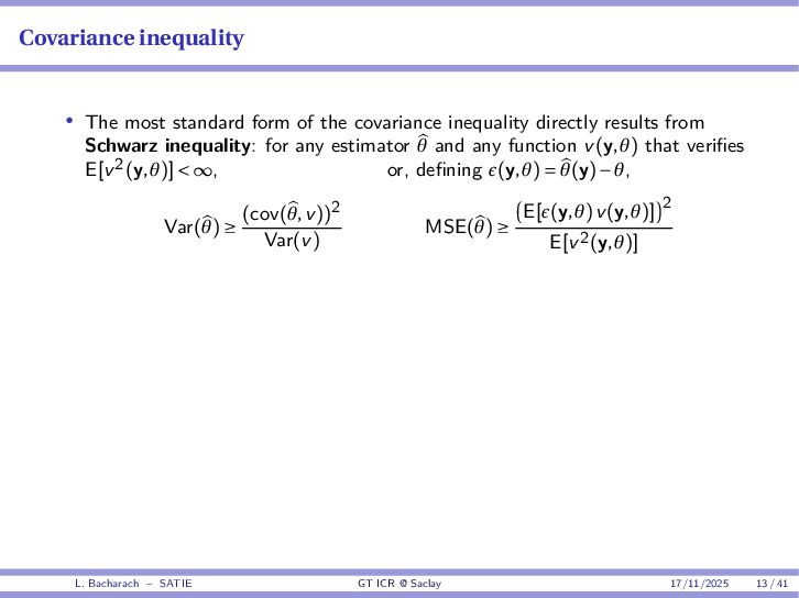
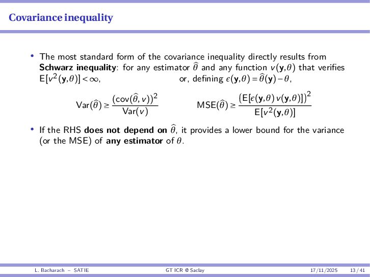
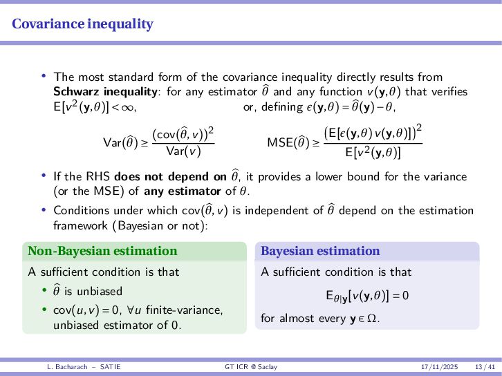
33. Covariance inequality • The most standard form of the covariance inequality directly results from Schwarz inequality: for any estimator θ and any function v(y,θ) that verifies E[v2(y,θ)] < ∞, or, defining ϵ(y,θ) = θ(y)−θ, Var(θ) ≥ (cov(θ,v))2 Var(v) MSE(θ) ≥ E[ϵ(y,θ)v(y,θ)] 2 E[v2(y,θ)] • If the RHS does not depend on θ, it provides a lower bound for the variance (or the MSE) of any estimator of θ. L. Bacharach – SATIE GT ICR @ Saclay 17/11/2025 13 / 41
34. Covariance inequality • The most standard form of the covariance inequality directly results from Schwarz inequality: for any estimator θ and any function v(y,θ) that verifies E[v2(y,θ)] < ∞, or, defining ϵ(y,θ) = θ(y)−θ, Var(θ) ≥ (cov(θ,v))2 Var(v) MSE(θ) ≥ E[ϵ(y,θ)v(y,θ)] 2 E[v2(y,θ)] • If the RHS does not depend on θ, it provides a lower bound for the variance (or the MSE) of any estimator of θ. • Conditions under which cov(θ,v) is independent of θ depend on the estimation framework (Bayesian or not): Non-Bayesian estimation A sufficient condition is that • θ is unbiased • cov(u,v) = 0, ∀u finite-variance, unbiased estimator of 0. Bayesian estimation A sufficient condition is that Eθ|y[v(y,θ)] = 0 for almost every y ∈ Ω. L. Bacharach – SATIE GT ICR @ Saclay 17/11/2025 13 / 41
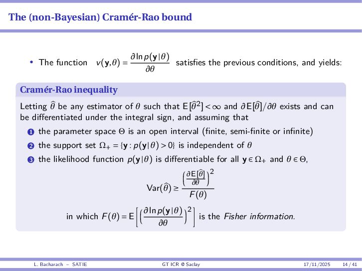
35. The (non-Bayesian) Cramér-Rao bound • The function v(y,θ) = ∂lnp(y|θ) ∂θ satisfies the previous conditions, and yields: Cramér-Rao inequality Letting θ be any estimator of θ such that E[θ2] < ∞ and ∂E[θ]/∂θ exists and can be differentiated under the integral sign, and assuming that 1 the parameter space Θ is an open interval (finite, semi-finite or infinite) 2 the support set Ω+ = {y : p(y|θ) > 0} is independent of θ 3 the likelihood function p(y|θ) is differentiable for all y ∈ Ω+ and θ ∈ Θ, Var(θ) ≥ ∂E[θ] ∂θ 2 F(θ) in which F(θ) = E ∂lnp(y|θ) ∂θ 2 is the Fisher information. L. Bacharach – SATIE GT ICR @ Saclay 17/11/2025 14 / 41
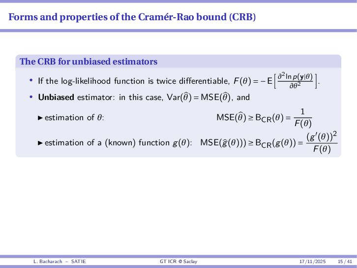
36. Forms and properties of the Cramér-Rao bound (CRB) The CRB for unbiased estimators • If the log-likelihood function is twice differentiable, F(θ) = −E ∂2 lnp(y|θ) ∂θ2 . • Unbiased estimator: in this case, Var(θ) = MSE(θ), and estimation of θ: MSE(θ) ≥ BCR(θ) = 1 F(θ) estimation of a (known) function g(θ): MSE(g(θ))) ≥ BCR(g(θ)) = (g′(θ))2 F(θ) L. Bacharach – SATIE GT ICR @ Saclay 17/11/2025 15 / 41
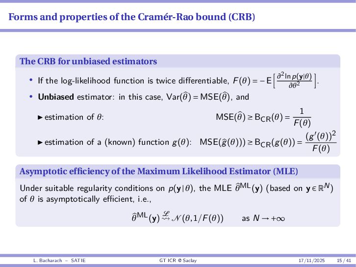
37. Forms and properties of the Cramér-Rao bound (CRB) The CRB for unbiased estimators • If the log-likelihood function is twice differentiable, F(θ) = −E ∂2 lnp(y|θ) ∂θ2 . • Unbiased estimator: in this case, Var(θ) = MSE(θ), and estimation of θ: MSE(θ) ≥ BCR(θ) = 1 F(θ) estimation of a (known) function g(θ): MSE(g(θ))) ≥ BCR(g(θ)) = (g′(θ))2 F(θ) Asymptotic efficiency of the Maximum Likelihood Estimator (MLE) Under suitable regularity conditions on p(y|θ), the MLE θML(y) (based on y ∈ RN) of θ is asymptotically efficient, i.e., θML(y) L ⇝ N (θ,1/F(θ)) as N → +∞ L. Bacharach – SATIE GT ICR @ Saclay 17/11/2025 15 / 41
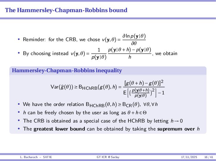
38. The Hammersley-Chapman-Robbins bound • Reminder: for the CRB, we chose v(y,θ) = ∂lnp(y|θ) ∂θ • By choosing instead v(y,θ) = 1 p(y|θ) p(y|θ +h)−p(y|θ) h , we obtain Hammersley-Chapman-Robbins inequality Var(g(θ)) ≥ BHChRB(g(θ),h) = [g(θ +h)−g(θ)]2 E p(y|θ+h) p(y|θ) 2 −1 • We have the order relation BHChRB(θ,h) ≥ BCR(θ), ∀θ,∀h • h can be freely chosen by the user as long as θ +h ∈ Θ • The CRB is obtained as a special case of the HChRB by letting h → 0 • The greatest lower bound can be obtained by taking the supremum over h L. Bacharach – SATIE GT ICR @ Saclay 17/11/2025 16 / 41
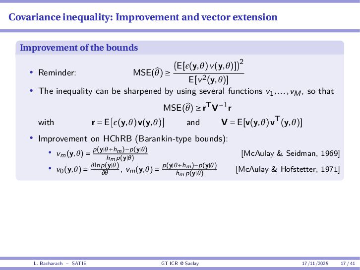
39. Covariance inequality: Improvement and vector extension Improvement of the bounds • Reminder: MSE(θ) ≥ E[ϵ(y,θ)v(y,θ)] 2 E[v2(y,θ)] • The inequality can be sharpened by using several functions v1,...,vM, so that MSE(θ) ≥ rTV−1r with r = E ϵ(y,θ)v(y,θ) and V = E[v(y,θ)vT(y,θ)] • Improvement on HChRB (Barankin-type bounds): • vm(y,θ) = p(y|θ+hm)−p(y|θ) hm p(y|θ) [McAulay & Seidman, 1969] • v0(y,θ) = ∂lnp(y|θ) ∂θ , vm(y,θ) = p(y|θ+hm)−p(y|θ) hm p(y|θ) [McAulay & Hofstetter, 1971] L. Bacharach – SATIE GT ICR @ Saclay 17/11/2025 17 / 41
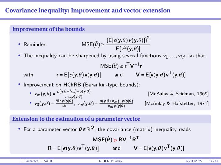
40. Covariance inequality: Improvement and vector extension Improvement of the bounds • Reminder: MSE(θ) ≥ E[ϵ(y,θ)v(y,θ)] 2 E[v2(y,θ)] • The inequality can be sharpened by using several functions v1,...,vM, so that MSE(θ) ≥ rTV−1r with r = E ϵ(y,θ)v(y,θ) and V = E[v(y,θ)vT(y,θ)] • Improvement on HChRB (Barankin-type bounds): • vm(y,θ) = p(y|θ+hm)−p(y|θ) hm p(y|θ) [McAulay & Seidman, 1969] • v0(y,θ) = ∂lnp(y|θ) ∂θ , vm(y,θ) = p(y|θ+hm)−p(y|θ) hm p(y|θ) [McAulay & Hofstetter, 1971] Extension to the estimation of a parameter vector • For a parameter vector θ ∈ RQ, the covariance (matrix) inequality reads MSE(θ) ≽ RV−1RT R = E ϵ(y,θ)vT(y,θ) and V = E[v(y,θ)vT(y,θ)] L. Bacharach – SATIE GT ICR @ Saclay 17/11/2025 17 / 41
41. Outline 1 Contexte Interféométrie radio Projet ANR PerDRIX : partenaires et problèmes traités 2 Bornes d’erreur d’estimation pour le placement des antennes Bornes inférieures de l’erreur quadratique moyenne (du MSE) classiques Exemple : estimation de la fréquence d’un signal sinusoïdal (complexe) Bornes d’erreur pour le placement d’antennes Vers des bornes plus pertinentes pour le placement des antennes ? 3 Conclusions, perspectives L. Bacharach – SATIE GT ICR @ Saclay 17/11/2025 18 / 41
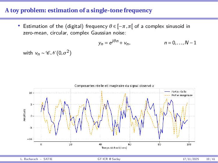
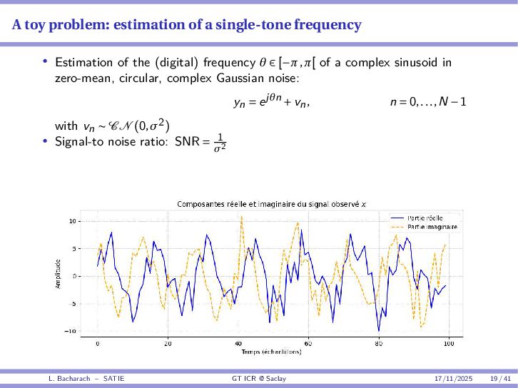
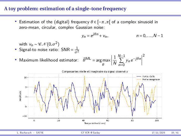
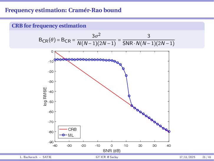
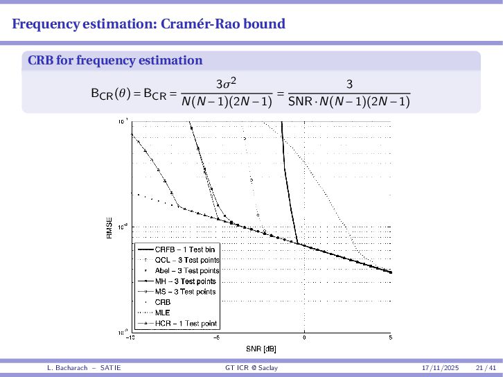
42. A toy problem: estimation of a single-tone frequency • Estimation of the (digital) frequency θ ∈ [−π,π[ of a complex sinusoid in zero-mean, circular, complex Gaussian noise: yn = ejθn +vn, n = 0,...,N −1 with vn ∼ C N (0,σ2) L. Bacharach – SATIE GT ICR @ Saclay 17/11/2025 19 / 41
43. A toy problem: estimation of a single-tone frequency • Estimation of the (digital) frequency θ ∈ [−π,π[ of a complex sinusoid in zero-mean, circular, complex Gaussian noise: yn = ejθn +vn, n = 0,...,N −1 with vn ∼ C N (0,σ2) • Signal-to noise ratio: SNR = 1 σ2 L. Bacharach – SATIE GT ICR @ Saclay 17/11/2025 19 / 41
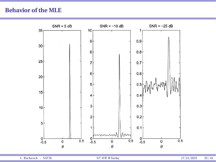
44. A toy problem: estimation of a single-tone frequency • Estimation of the (digital) frequency θ ∈ [−π,π[ of a complex sinusoid in zero-mean, circular, complex Gaussian noise: yn = ejθn +vn, n = 0,...,N −1 with vn ∼ C N (0,σ2) • Signal-to noise ratio: SNR = 1 σ2 • Maximum likelihood estimator: θML = argmax θ 1 N N−1 n=0 yn e−jθn 2 L. Bacharach – SATIE GT ICR @ Saclay 17/11/2025 19 / 41
45. Behavior of the MLE L. Bacharach – SATIE GT ICR @ Saclay 17/11/2025 20 / 41
46. Frequency estimation: Cramér-Rao bound CRB for frequency estimation BCR(θ) = BCR = 3σ2 N(N −1)(2N −1) = 3 SNR·N(N −1)(2N −1) -40 -30 -20 -10 0 10 20 30 40 -90 -80 -70 -60 -50 -40 -30 -20 -10 0 CRB ML SNR (dB) log RMSE L. Bacharach – SATIE GT ICR @ Saclay 17/11/2025 21 / 41
47. Frequency estimation: Cramér-Rao bound CRB for frequency estimation BCR(θ) = BCR = 3σ2 N(N −1)(2N −1) = 3 SNR·N(N −1)(2N −1) L. Bacharach – SATIE GT ICR @ Saclay 17/11/2025 21 / 41
48. Outline 1 Contexte Interféométrie radio Projet ANR PerDRIX : partenaires et problèmes traités 2 Bornes d’erreur d’estimation pour le placement des antennes Bornes inférieures de l’erreur quadratique moyenne (du MSE) classiques Exemple : estimation de la fréquence d’un signal sinusoïdal (complexe) Bornes d’erreur pour le placement d’antennes Vers des bornes plus pertinentes pour le placement des antennes ? 3 Conclusions, perspectives L. Bacharach – SATIE GT ICR @ Saclay 17/11/2025 22 / 41
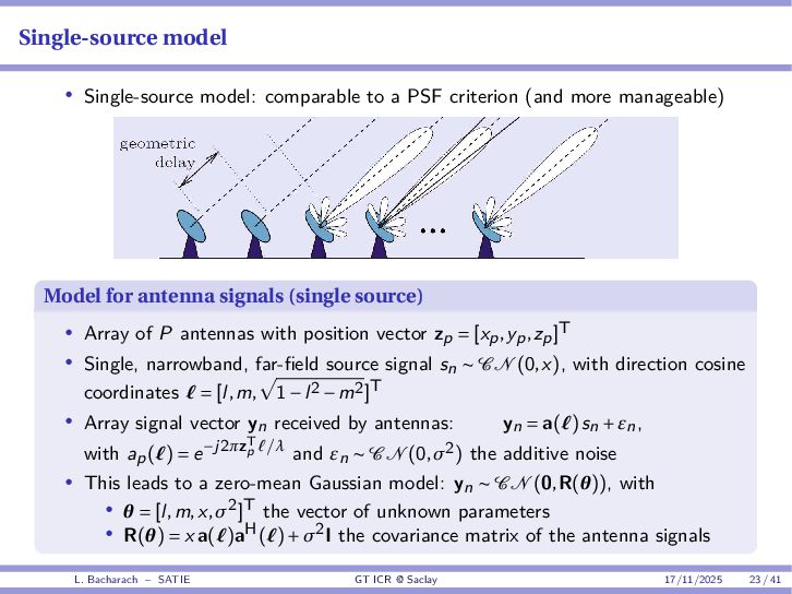
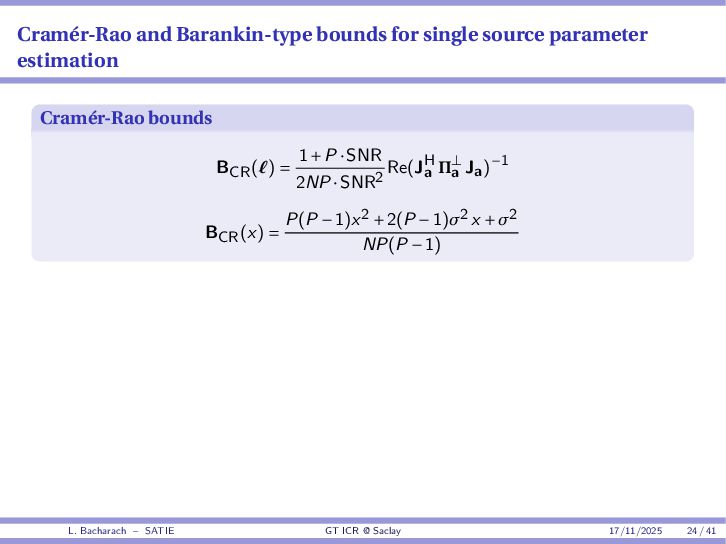
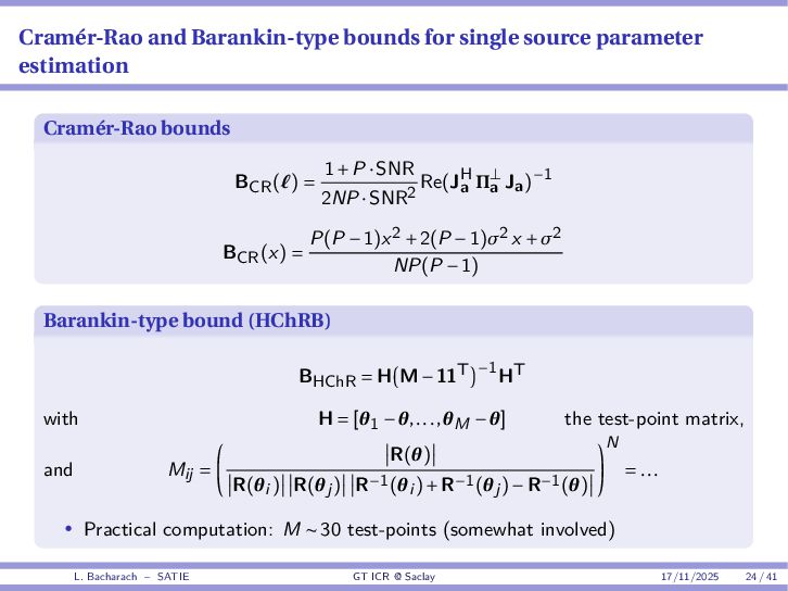
49. Single-source model • Single-source model: comparable to a PSF criterion (and more manageable) Model for antenna signals (single source) • Array of P antennas with position vector zp = [xp,yp,zp]T • Single, narrowband, far-field source signal sn ∼ C N (0,x), with direction cosine coordinates ℓ = [l,m, 1−l2 −m2]T • Array signal vector yn received by antennas: yn = a(ℓ)sn +εn, with ap(ℓ) = e−j2πzT p ℓ/λ and εn ∼ C N (0,σ2) the additive noise • This leads to a zero-mean Gaussian model: yn ∼ C N (0,R(θ)), with • θ = [l,m,x,σ2]T the vector of unknown parameters • R(θ) = x a(ℓ)aH(ℓ)+σ2I the covariance matrix of the antenna signals L. Bacharach – SATIE GT ICR @ Saclay 17/11/2025 23 / 41
50. Cramér-Rao and Barankin-type bounds for single source parameter estimation Cramér-Rao bounds BCR(ℓ) = 1+P ·SNR 2NP ·SNR2 Re(JH a Π⊥ a Ja)−1 BCR(x) = P(P −1)x2 +2(P −1)σ2 x +σ2 NP(P −1) L. Bacharach – SATIE GT ICR @ Saclay 17/11/2025 24 / 41
51. Cramér-Rao and Barankin-type bounds for single source parameter estimation Cramér-Rao bounds BCR(ℓ) = 1+P ·SNR 2NP ·SNR2 Re(JH a Π⊥ a Ja)−1 BCR(x) = P(P −1)x2 +2(P −1)σ2 x +σ2 NP(P −1) Barankin-type bound (HChRB) BHChR = H M−11T −1HT with H = [θ1 −θ,...,θM −θ] the test-point matrix, and Mij = R(θ) R(θi ) R(θj) R−1(θi )+R−1(θj)−R−1(θ) N = ... • Practical computation: M ∼ 30 test-points (somewhat involved) L. Bacharach – SATIE GT ICR @ Saclay 17/11/2025 24 / 41
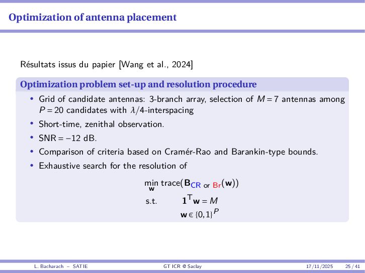
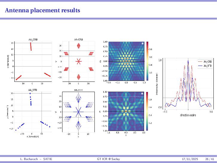
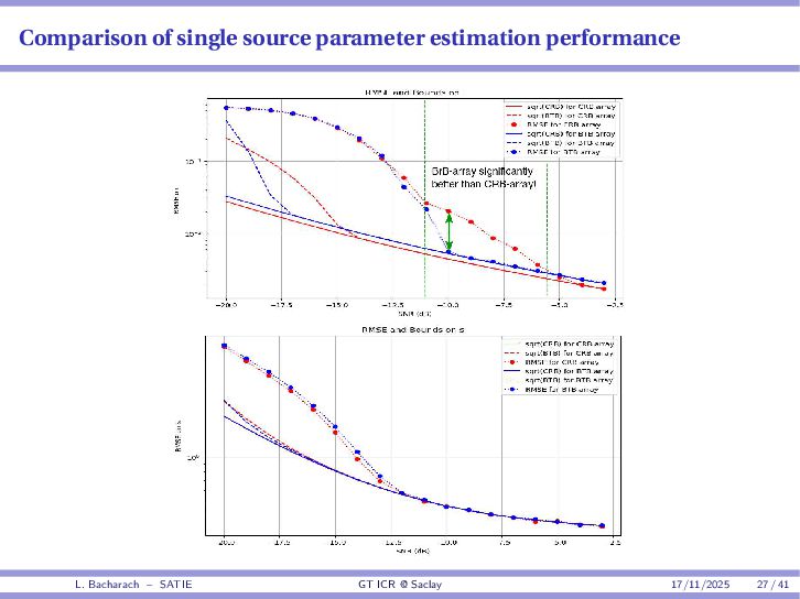
52. Optimization of antenna placement Résultats issus du papier [Wang et al., 2024] Optimization problem set-up and resolution procedure • Grid of candidate antennas: 3-branch array, selection of M = 7 antennas among P = 20 candidates with λ/4-interspacing • Short-time, zenithal observation. • SNR = −12 dB. • Comparison of criteria based on Cramér-Rao and Barankin-type bounds. • Exhaustive search for the resolution of min w trace(BCR or Br(w)) s.t. 1Tw = M w ∈ {0,1}P L. Bacharach – SATIE GT ICR @ Saclay 17/11/2025 25 / 41
53. Antenna placement results L. Bacharach – SATIE GT ICR @ Saclay 17/11/2025 26 / 41
54. Comparison of single source parameter estimation performance L. Bacharach – SATIE GT ICR @ Saclay 17/11/2025 27 / 41
55. uv-plane coverage and imaging performance over a 4-hour observation L. Bacharach – SATIE GT ICR @ Saclay 17/11/2025 28 / 41
56. Limitations of the approach and ongoing work (in radio interferometry) Limitations of the current approach • The criterion used: trace(Bound), and thus its minimum... L. Bacharach – SATIE GT ICR @ Saclay 17/11/2025 29 / 41
57. Limitations of the approach and ongoing work (in radio interferometry) Limitations of the current approach • The criterion used: trace(Bound), and thus its minimum... depend on the true value of the unknown parameter θ (in particular the SNR) indistinctly adds errors on parameters of different natures: (l,m) VS x L. Bacharach – SATIE GT ICR @ Saclay 17/11/2025 29 / 41
58. Limitations of the approach and ongoing work (in radio interferometry) Limitations of the current approach • The criterion used: trace(Bound), and thus its minimum... depend on the true value of the unknown parameter θ (in particular the SNR) indistinctly adds errors on parameters of different natures: (l,m) VS x → Does a more appropriate criterion exist? L. Bacharach – SATIE GT ICR @ Saclay 17/11/2025 29 / 41
59. Limitations of the approach and ongoing work (in radio interferometry) Limitations of the current approach • The criterion used: trace(Bound), and thus its minimum... depend on the true value of the unknown parameter θ (in particular the SNR) indistinctly adds errors on parameters of different natures: (l,m) VS x → Does a more appropriate criterion exist? • Barankin bound: relevant, but computationally burdensome... L. Bacharach – SATIE GT ICR @ Saclay 17/11/2025 29 / 41
60. Limitations of the approach and ongoing work (in radio interferometry) Limitations of the current approach • The criterion used: trace(Bound), and thus its minimum... depend on the true value of the unknown parameter θ (in particular the SNR) indistinctly adds errors on parameters of different natures: (l,m) VS x → Does a more appropriate criterion exist? • Barankin bound: relevant, but computationally burdensome... • Small-dimensional antenna selection (exhaustive search) L. Bacharach – SATIE GT ICR @ Saclay 17/11/2025 29 / 41
61. Limitations of the approach and ongoing work (in radio interferometry) Limitations of the current approach • The criterion used: trace(Bound), and thus its minimum... depend on the true value of the unknown parameter θ (in particular the SNR) indistinctly adds errors on parameters of different natures: (l,m) VS x → Does a more appropriate criterion exist? • Barankin bound: relevant, but computationally burdensome... • Small-dimensional antenna selection (exhaustive search) • The model considers: isotropic antennas a single source, a single frequency band received antenna signals, instead of the actual interferometric model (visibilities) L. Bacharach – SATIE GT ICR @ Saclay 17/11/2025 29 / 41
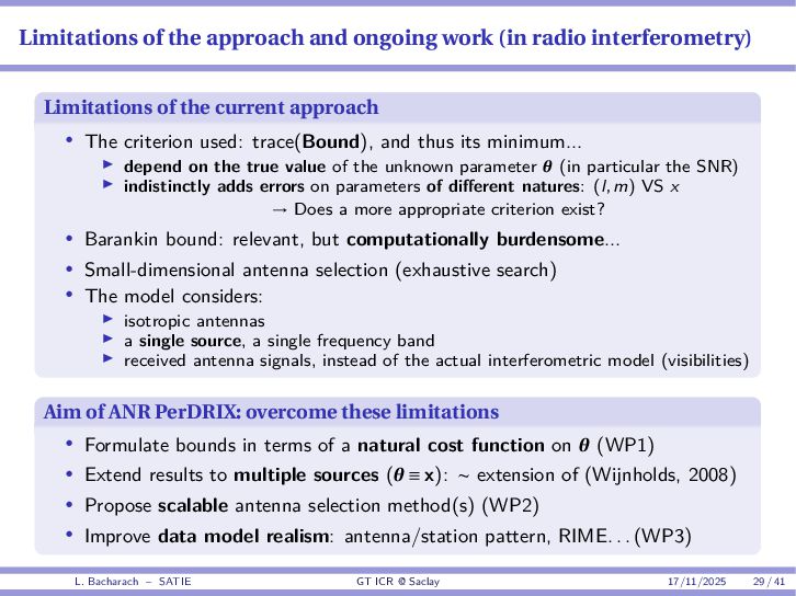
62. Limitations of the approach and ongoing work (in radio interferometry) Limitations of the current approach • The criterion used: trace(Bound), and thus its minimum... depend on the true value of the unknown parameter θ (in particular the SNR) indistinctly adds errors on parameters of different natures: (l,m) VS x → Does a more appropriate criterion exist? • Barankin bound: relevant, but computationally burdensome... • Small-dimensional antenna selection (exhaustive search) • The model considers: isotropic antennas a single source, a single frequency band received antenna signals, instead of the actual interferometric model (visibilities) Aim of ANR PerDRIX: overcome these limitations • Formulate bounds in terms of a natural cost function on θ (WP1) • Extend results to multiple sources (θ ≡ x): ∼ extension of (Wijnholds, 2008) • Propose scalable antenna selection method(s) (WP2) • Improve data model realism: antenna/station pattern, RIME. . . (WP3) L. Bacharach – SATIE GT ICR @ Saclay 17/11/2025 29 / 41
63. Outline 1 Contexte Interféométrie radio Projet ANR PerDRIX : partenaires et problèmes traités 2 Bornes d’erreur d’estimation pour le placement des antennes Bornes inférieures de l’erreur quadratique moyenne (du MSE) classiques Exemple : estimation de la fréquence d’un signal sinusoïdal (complexe) Bornes d’erreur pour le placement d’antennes Vers des bornes plus pertinentes pour le placement des antennes ? 3 Conclusions, perspectives L. Bacharach – SATIE GT ICR @ Saclay 17/11/2025 30 / 41
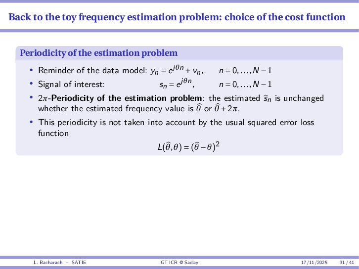
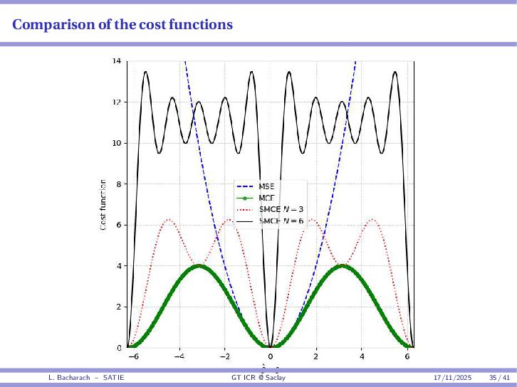
64. Back to the toy frequency estimation problem: choice of the cost function Periodicity of the estimation problem • Reminder of the data model: yn = ejθn +vn, n = 0,...,N −1 • Signal of interest: sn = ejθn, n = 0,...,N −1 • 2π-Periodicity of the estimation problem: the estimated sn is unchanged whether the estimated frequency value is θ or θ +2π. • This periodicity is not taken into account by the usual squared error loss function L(θ,θ) = (θ −θ)2 L. Bacharach – SATIE GT ICR @ Saclay 17/11/2025 31 / 41
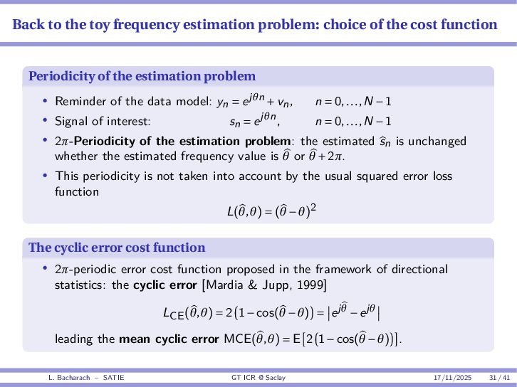
65. Back to the toy frequency estimation problem: choice of the cost function Periodicity of the estimation problem • Reminder of the data model: yn = ejθn +vn, n = 0,...,N −1 • Signal of interest: sn = ejθn, n = 0,...,N −1 • 2π-Periodicity of the estimation problem: the estimated sn is unchanged whether the estimated frequency value is θ or θ +2π. • This periodicity is not taken into account by the usual squared error loss function L(θ,θ) = (θ −θ)2 The cyclic error cost function • 2π-periodic error cost function proposed in the framework of directional statistics: the cyclic error [Mardia & Jupp, 1999] LCE(θ,θ) = 2 1−cos(θ −θ) = ejθ −ejθ leading the mean cyclic error MCE(θ,θ) = E 2 1−cos(θ −θ) . L. Bacharach – SATIE GT ICR @ Saclay 17/11/2025 31 / 41
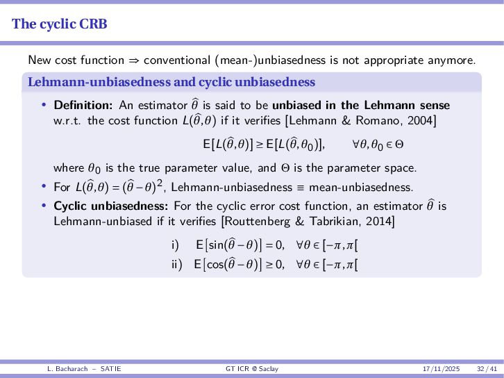
66. The cyclic CRB New cost function ⇒ conventional (mean-)unbiasedness is not appropriate anymore. Lehmann-unbiasedness and cyclic unbiasedness • Definition: An estimator θ is said to be unbiased in the Lehmann sense w.r.t. the cost function L(θ,θ) if it verifies [Lehmann & Romano, 2004] E[L(θ,θ)] ≥ E[L(θ,θ0)], ∀θ,θ0 ∈ Θ where θ0 is the true parameter value, and Θ is the parameter space. • For L(θ,θ) = (θ −θ)2, Lehmann-unbiasedness ≡ mean-unbiasedness. • Cyclic unbiasedness: For the cyclic error cost function, an estimator θ is Lehmann-unbiased if it verifies [Routtenberg & Tabrikian, 2014] i) E sin(θ −θ) = 0, ∀θ ∈ [−π,π[ ii) E cos(θ −θ) ≥ 0, ∀θ ∈ [−π,π[ L. Bacharach – SATIE GT ICR @ Saclay 17/11/2025 32 / 41
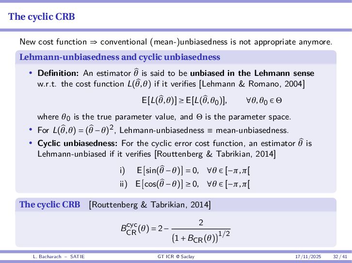
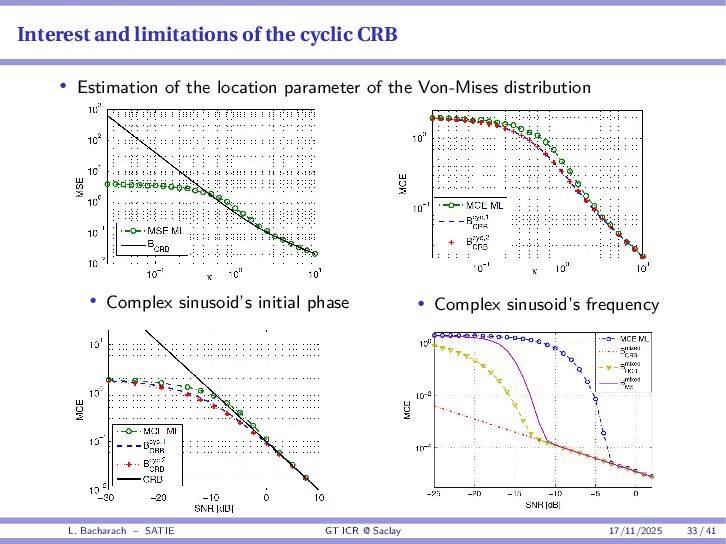
67. The cyclic CRB New cost function ⇒ conventional (mean-)unbiasedness is not appropriate anymore. Lehmann-unbiasedness and cyclic unbiasedness • Definition: An estimator θ is said to be unbiased in the Lehmann sense w.r.t. the cost function L(θ,θ) if it verifies [Lehmann & Romano, 2004] E[L(θ,θ)] ≥ E[L(θ,θ0)], ∀θ,θ0 ∈ Θ where θ0 is the true parameter value, and Θ is the parameter space. • For L(θ,θ) = (θ −θ)2, Lehmann-unbiasedness ≡ mean-unbiasedness. • Cyclic unbiasedness: For the cyclic error cost function, an estimator θ is Lehmann-unbiased if it verifies [Routtenberg & Tabrikian, 2014] i) E sin(θ −θ) = 0, ∀θ ∈ [−π,π[ ii) E cos(θ −θ) ≥ 0, ∀θ ∈ [−π,π[ The cyclic CRB [Routtenberg & Tabrikian, 2014] Bcyc CR (θ) = 2− 2 1+BCR(θ) 1/2 L. Bacharach – SATIE GT ICR @ Saclay 17/11/2025 32 / 41
68. Interest and limitations of the cyclic CRB • Estimation of the location parameter of the Von-Mises distribution L. Bacharach – SATIE GT ICR @ Saclay 17/11/2025 33 / 41
69. Interest and limitations of the cyclic CRB • Estimation of the location parameter of the Von-Mises distribution • Complex sinusoid’s initial phase L. Bacharach – SATIE GT ICR @ Saclay 17/11/2025 33 / 41
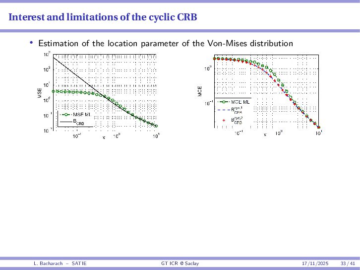
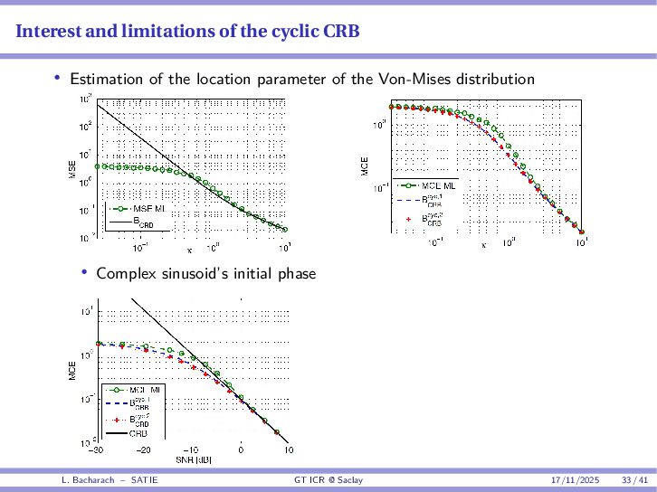
70. Interest and limitations of the cyclic CRB • Estimation of the location parameter of the Von-Mises distribution • Complex sinusoid’s initial phase • Complex sinusoid’s frequency L. Bacharach – SATIE GT ICR @ Saclay 17/11/2025 33 / 41
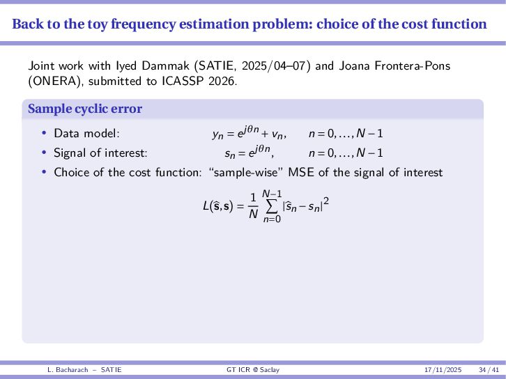
71. Back to the toy frequency estimation problem: choice of the cost function Joint work with Iyed Dammak (SATIE, 2025/04–07) and Joana Frontera-Pons (ONERA), submitted to ICASSP 2026. Sample cyclic error • Data model: yn = ejθn +vn, n = 0,...,N −1 • Signal of interest: sn = ejθn, n = 0,...,N −1 • Choice of the cost function: “sample-wise” MSE of the signal of interest L(s,s) = 1 N N−1 n=0 |sn −sn|2 L. Bacharach – SATIE GT ICR @ Saclay 17/11/2025 34 / 41
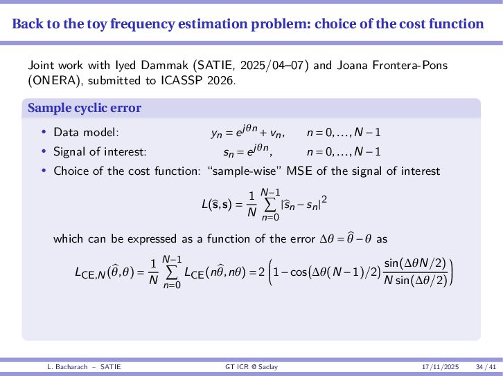
72. Back to the toy frequency estimation problem: choice of the cost function Joint work with Iyed Dammak (SATIE, 2025/04–07) and Joana Frontera-Pons (ONERA), submitted to ICASSP 2026. Sample cyclic error • Data model: yn = ejθn +vn, n = 0,...,N −1 • Signal of interest: sn = ejθn, n = 0,...,N −1 • Choice of the cost function: “sample-wise” MSE of the signal of interest L(s,s) = 1 N N−1 n=0 |sn −sn|2 which can be expressed as a function of the error ∆θ = θ −θ as LCE,N(θ,θ) = 1 N N−1 n=0 LCE(nθ,nθ) = 2 1−cos ∆θ(N −1)/2 sin(∆θN/2) N sin(∆θ/2) L. Bacharach – SATIE GT ICR @ Saclay 17/11/2025 34 / 41
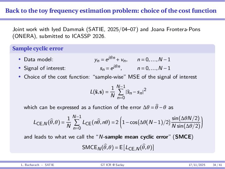
73. Back to the toy frequency estimation problem: choice of the cost function Joint work with Iyed Dammak (SATIE, 2025/04–07) and Joana Frontera-Pons (ONERA), submitted to ICASSP 2026. Sample cyclic error • Data model: yn = ejθn +vn, n = 0,...,N −1 • Signal of interest: sn = ejθn, n = 0,...,N −1 • Choice of the cost function: “sample-wise” MSE of the signal of interest L(s,s) = 1 N N−1 n=0 |sn −sn|2 which can be expressed as a function of the error ∆θ = θ −θ as LCE,N(θ,θ) = 1 N N−1 n=0 LCE(nθ,nθ) = 2 1−cos ∆θ(N −1)/2 sin(∆θN/2) N sin(∆θ/2) and leads to what we call the “N-sample mean cyclic error” (SMCE) SMCEN(θ,θ) = E LCE,N(θ,θ) L. Bacharach – SATIE GT ICR @ Saclay 17/11/2025 34 / 41
74. Comparison of the cost functions L. Bacharach – SATIE GT ICR @ Saclay 17/11/2025 35 / 41
75. Cramér-Rao bound for the sample mean cyclic error (SMCE) The “N-sample” cyclic CRB • It is relatively straightforward to obtain from the previous cyclic CRB: SMCEN(θ,θ) ≥ Bs-cyc CR,N (θ) = 1 N N−1 n=0 Bcyc CR (nθ) = 2  1− 1 N N−1 n=0 1 1+n2BCR(θ) 1/2   L. Bacharach – SATIE GT ICR @ Saclay 17/11/2025 36 / 41
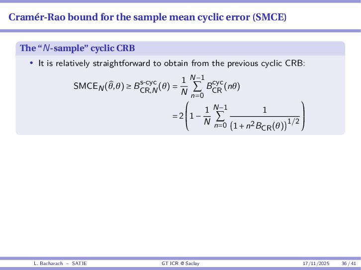
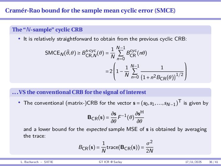
76. Cramér-Rao bound for the sample mean cyclic error (SMCE) The “N-sample” cyclic CRB • It is relatively straightforward to obtain from the previous cyclic CRB: SMCEN(θ,θ) ≥ Bs-cyc CR,N (θ) = 1 N N−1 n=0 Bcyc CR (nθ) = 2  1− 1 N N−1 n=0 1 1+n2BCR(θ) 1/2   ...VS the conventional CRB for the signal of interest • The conventional (matrix-)CRB for the vector s = (s0,s1,...,sN−1)T is given by BCR(s) = ∂s ∂θ F−1(θ) ∂sH ∂θ and a lower bound for the expected sample MSE of s is obtained by averaging the trace: BCR(s) = 1 N trace(BCR(s)) = σ2 2N L. Bacharach – SATIE GT ICR @ Saclay 17/11/2025 36 / 41
77. CRB for the SMCE: numerical result L. Bacharach – SATIE GT ICR @ Saclay 17/11/2025 37 / 41
78. Outline 1 Contexte Interféométrie radio Projet ANR PerDRIX : partenaires et problèmes traités 2 Bornes d’erreur d’estimation pour le placement des antennes Bornes inférieures de l’erreur quadratique moyenne (du MSE) classiques Exemple : estimation de la fréquence d’un signal sinusoïdal (complexe) Bornes d’erreur pour le placement d’antennes Vers des bornes plus pertinentes pour le placement des antennes ? 3 Conclusions, perspectives L. Bacharach – SATIE GT ICR @ Saclay 17/11/2025 38 / 41
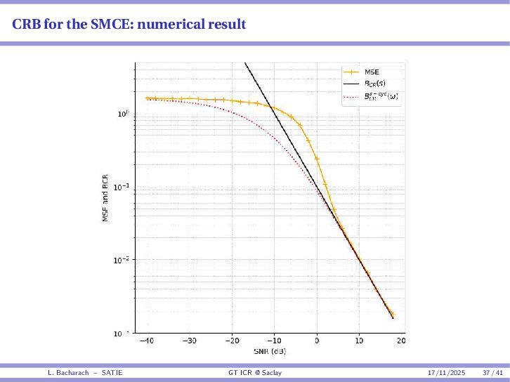
79. Concluding remarks and perspectives A few observations and concluding remarks • The threshold effect is less pronounced using the SMCE. • The CRB for the SMCE is more appropriate than the cyclic CRB (for the MCE) for frequency estimation. • The conventional CRB only provides insight on asymptotic performance. • The choice of the error cost function is fundamental. L. Bacharach – SATIE GT ICR @ Saclay 17/11/2025 39 / 41
80. Concluding remarks and perspectives A few observations and concluding remarks • The threshold effect is less pronounced using the SMCE. • The CRB for the SMCE is more appropriate than the cyclic CRB (for the MCE) for frequency estimation. • The conventional CRB only provides insight on asymptotic performance. • The choice of the error cost function is fundamental. Future work • Extension to the joint estimation of amplitude A, frequency θ and initial phase φ of a complex sinusoid: sn = Aej(nθ+φ) ⇒ a “mix” between conventional MSE for A, MCE for φ and SMCE for θ • Extension to single-source DOA estimation: nonuniform sampling, 2d-frequency • Application to the antenna placement problem (WP2), in particular in radio interferometry (WP3) ⇒ Post-doc position available soon! L. Bacharach – SATIE GT ICR @ Saclay 17/11/2025 39 / 41
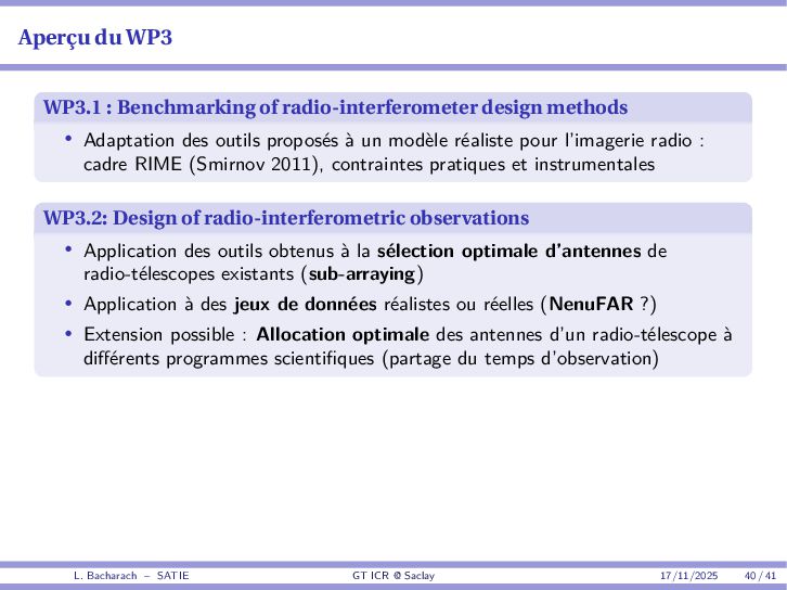
81. Aperçu du WP3 WP3.1 : Benchmarking of radio-interferometer design methods • Adaptation des outils proposés à un modèle réaliste pour l’imagerie radio : cadre RIME (Smirnov 2011), contraintes pratiques et instrumentales L. Bacharach – SATIE GT ICR @ Saclay 17/11/2025 40 / 41
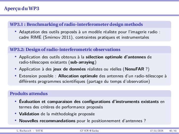
82. Aperçu du WP3 WP3.1 : Benchmarking of radio-interferometer design methods • Adaptation des outils proposés à un modèle réaliste pour l’imagerie radio : cadre RIME (Smirnov 2011), contraintes pratiques et instrumentales WP3.2: Design of radio-interferometric observations • Application des outils obtenus à la sélection optimale d’antennes de radio-télescopes existants (sub-arraying) • Application à des jeux de données réalistes ou réelles (NenuFAR ?) • Extension possible : Allocation optimale des antennes d’un radio-télescope à différents programmes scientifiques (partage du temps d’observation) L. Bacharach – SATIE GT ICR @ Saclay 17/11/2025 40 / 41
83. Aperçu du WP3 WP3.1 : Benchmarking of radio-interferometer design methods • Adaptation des outils proposés à un modèle réaliste pour l’imagerie radio : cadre RIME (Smirnov 2011), contraintes pratiques et instrumentales WP3.2: Design of radio-interferometric observations • Application des outils obtenus à la sélection optimale d’antennes de radio-télescopes existants (sub-arraying) • Application à des jeux de données réalistes ou réelles (NenuFAR ?) • Extension possible : Allocation optimale des antennes d’un radio-télescope à différents programmes scientifiques (partage du temps d’observation) Produits attendus • Évaluation et comparaison des configurations d’instruments existants en termes des critères de performance proposés • Validation de la méthodologie proposée • Nouvelles recommandations pour le positionnement d’antennes ? L. Bacharach – SATIE GT ICR @ Saclay 17/11/2025 40 / 41
84. Thank you for your attention! L. Bacharach – SATIE GT ICR @ Saclay 17/11/2025 41 / 41