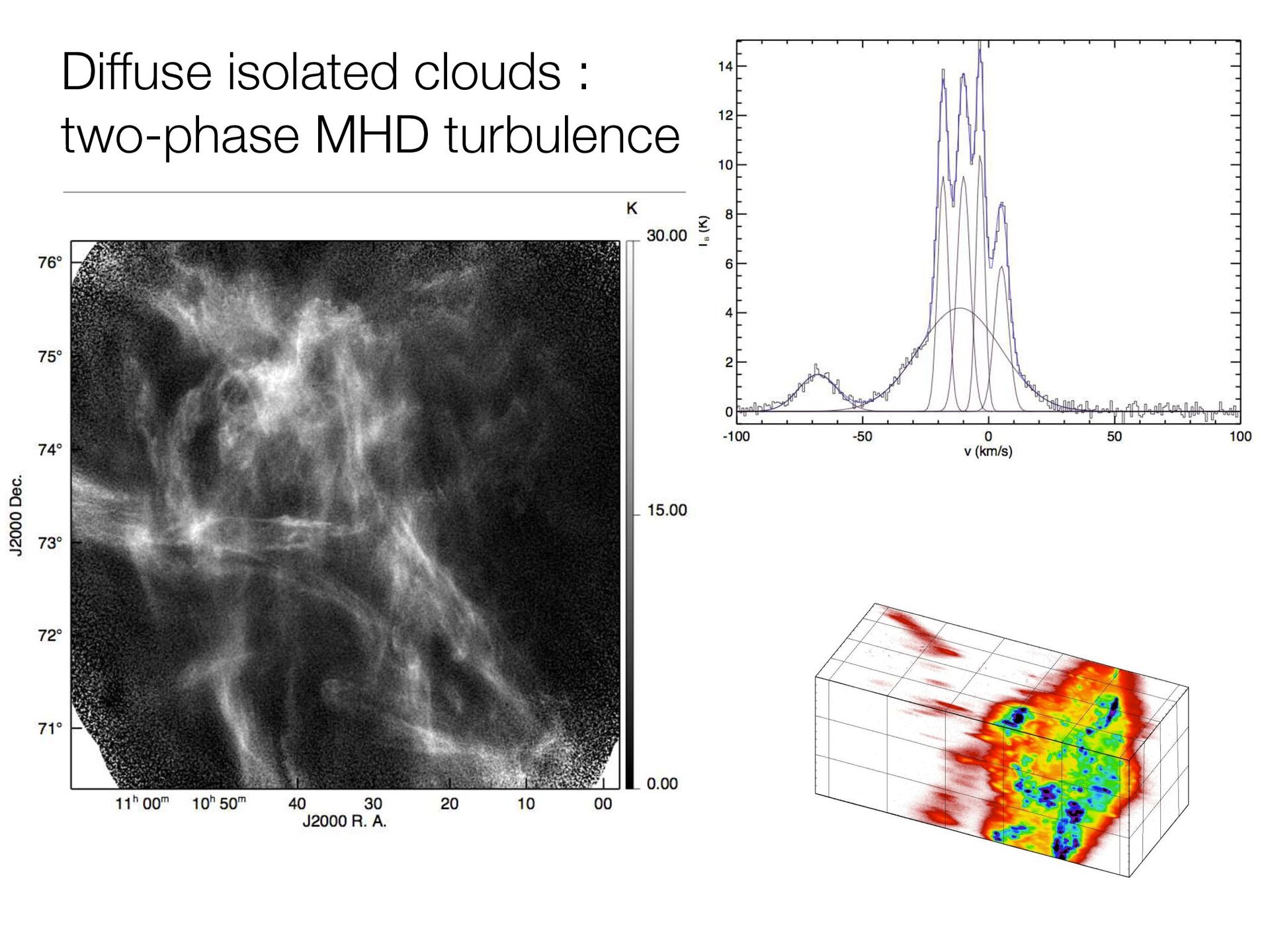
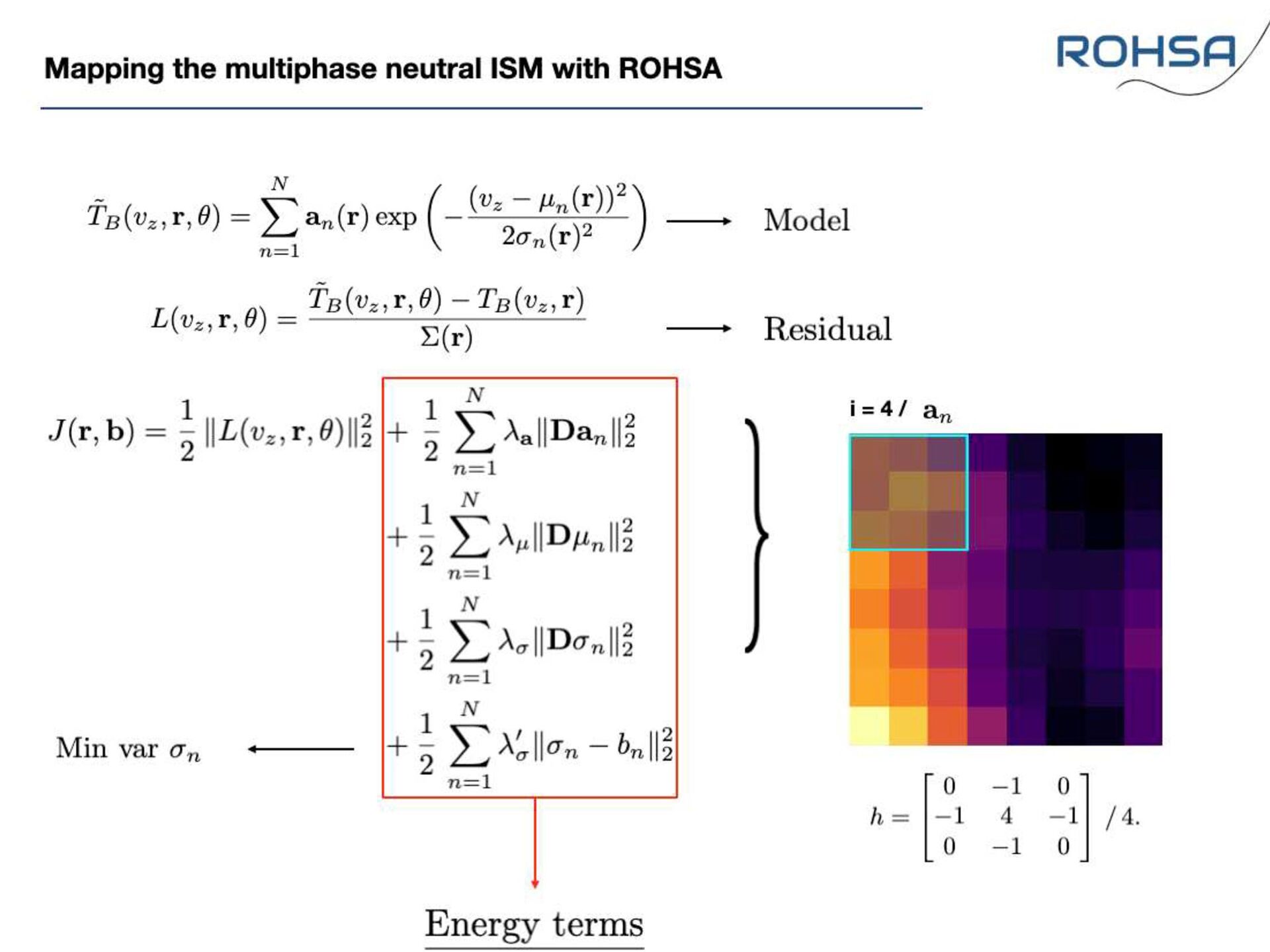
TB[x, y, v] Application on 21 cm observations of the North Ecliptic Pole field ROHSA : decomposition of emission on a Gaussian basis Marchal et al. (2019)
TB[x, y, v] Application on 21 cm observations of the North Ecliptic Pole field ROHSA : decomposition of emission on a Gaussian basis Marchal et al. (2019)
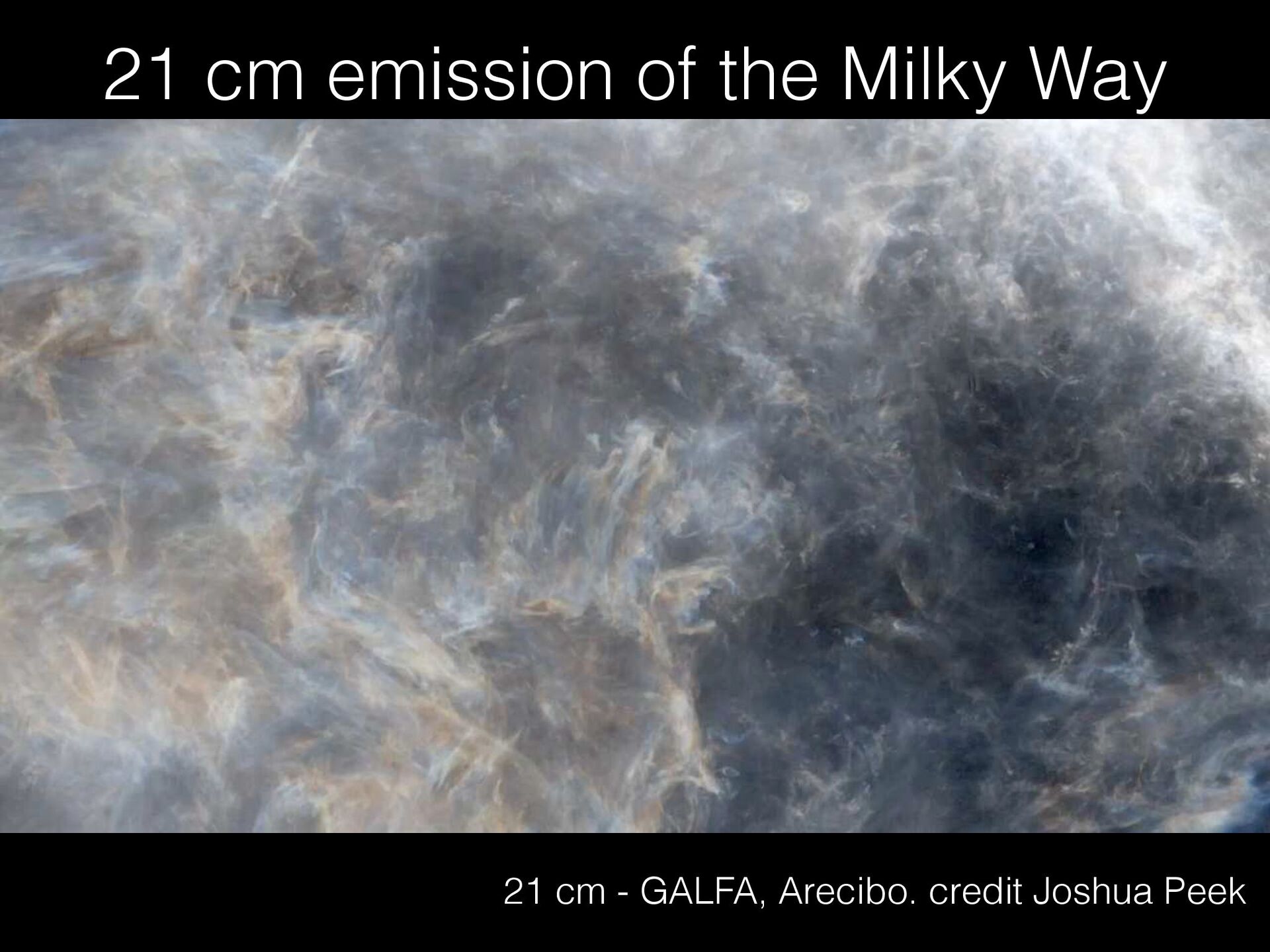
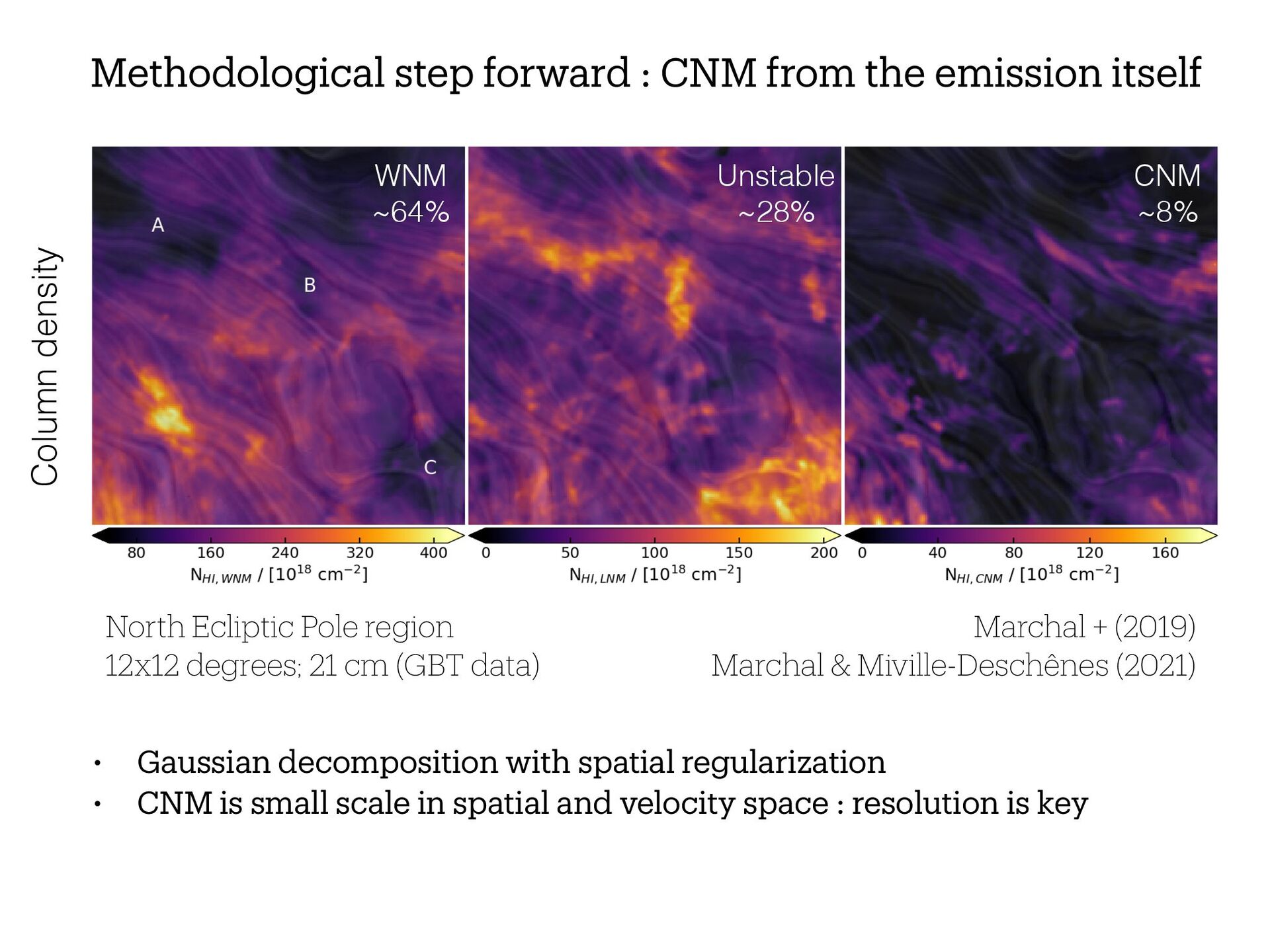
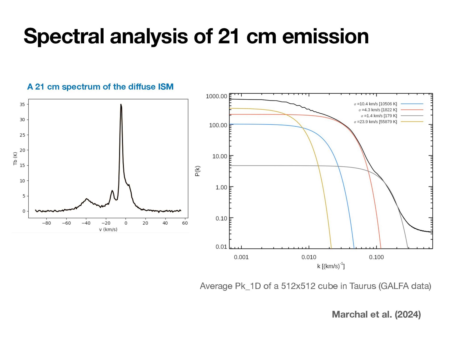
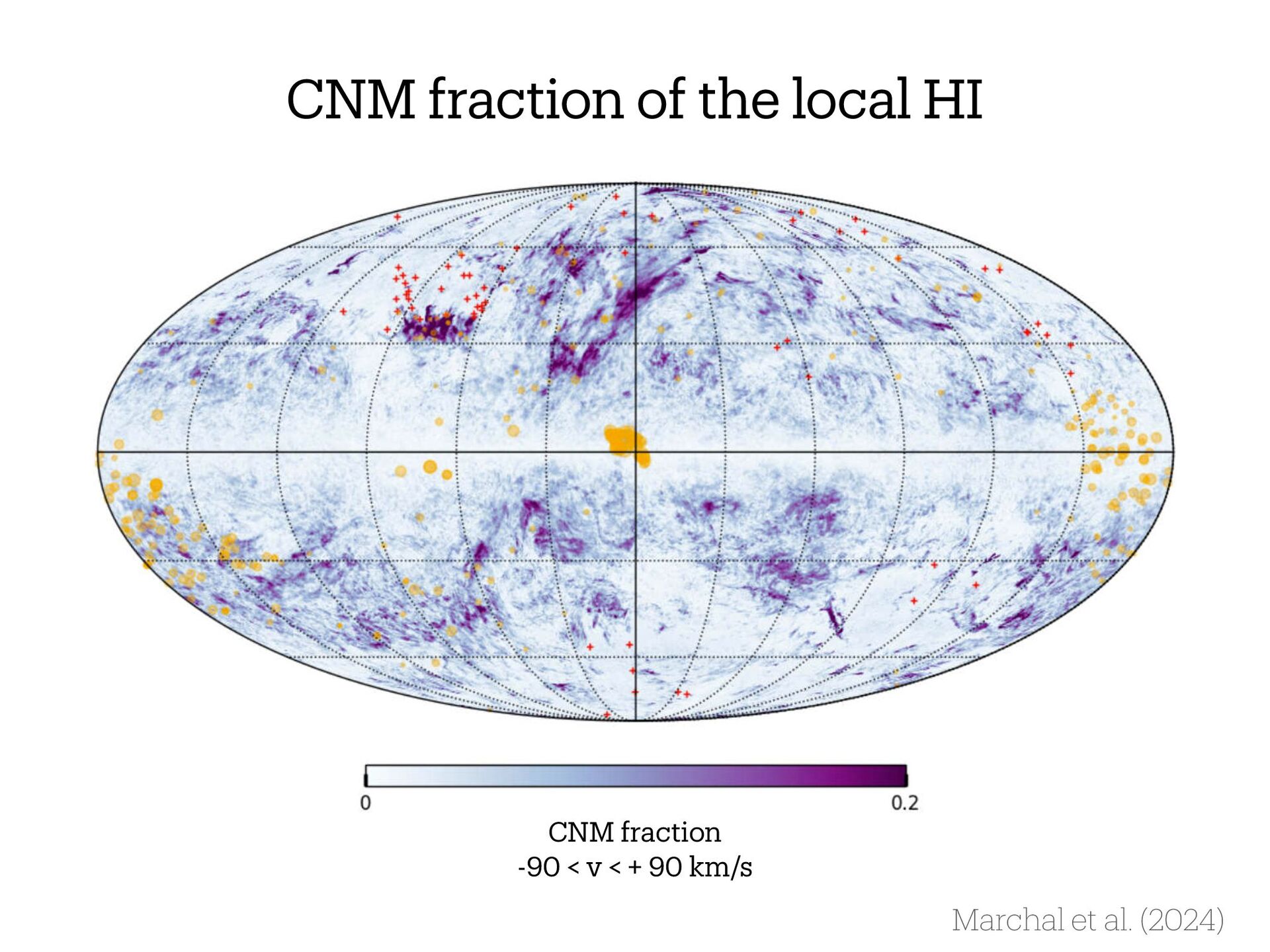
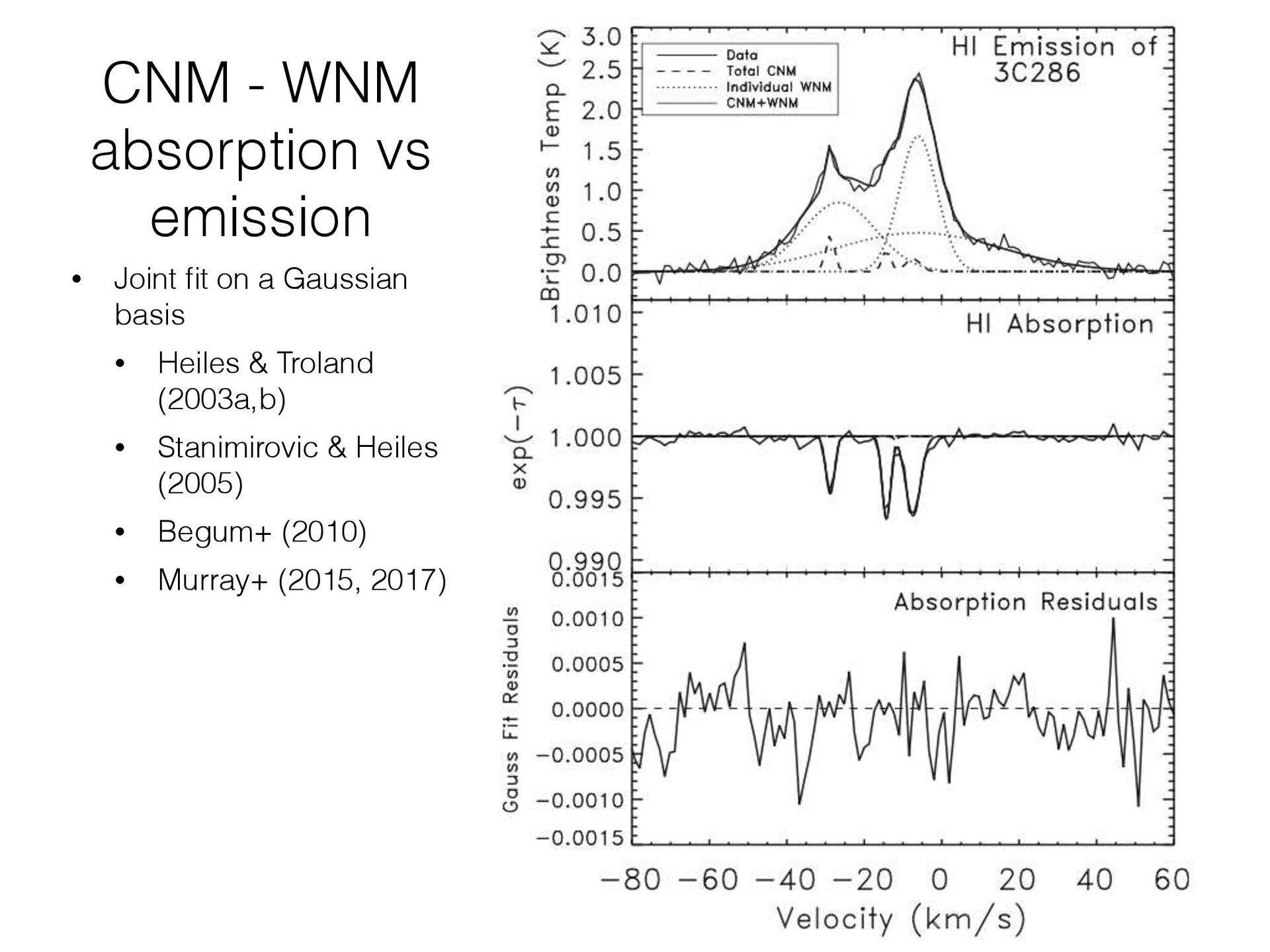
decomposition with spatial regularization • CNM is small scale in spatial and velocity space : resolution is key Marchal + (2019) Marchal & Miville-Deschênes (2021) North Ecliptic Pole region 12x12 degrees; 21 cm (GBT data) Methodological step forward : CNM from the emission itself
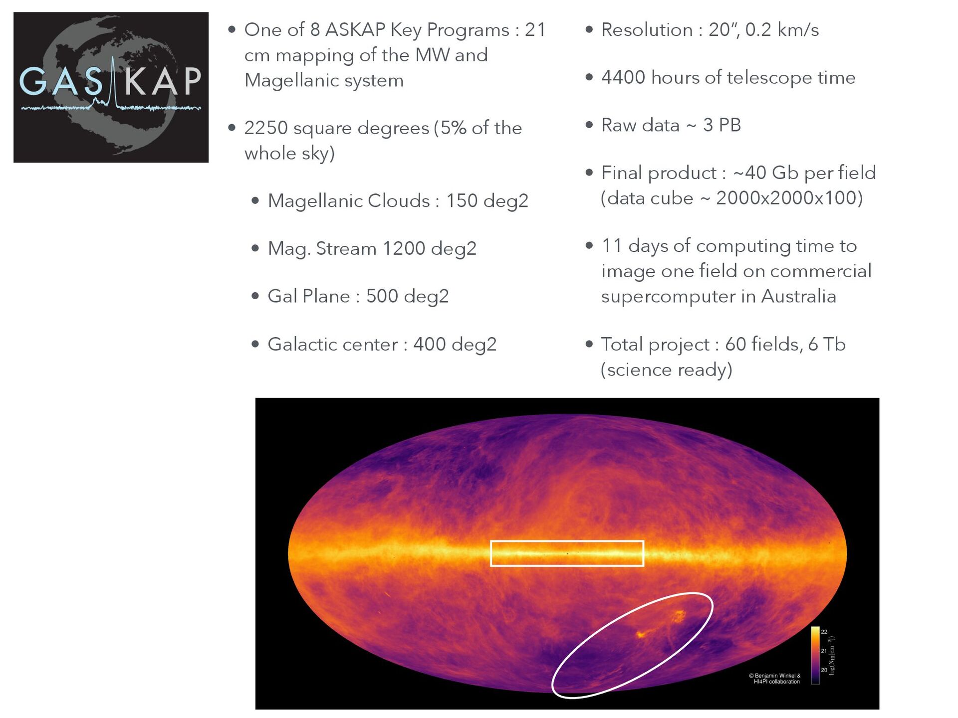
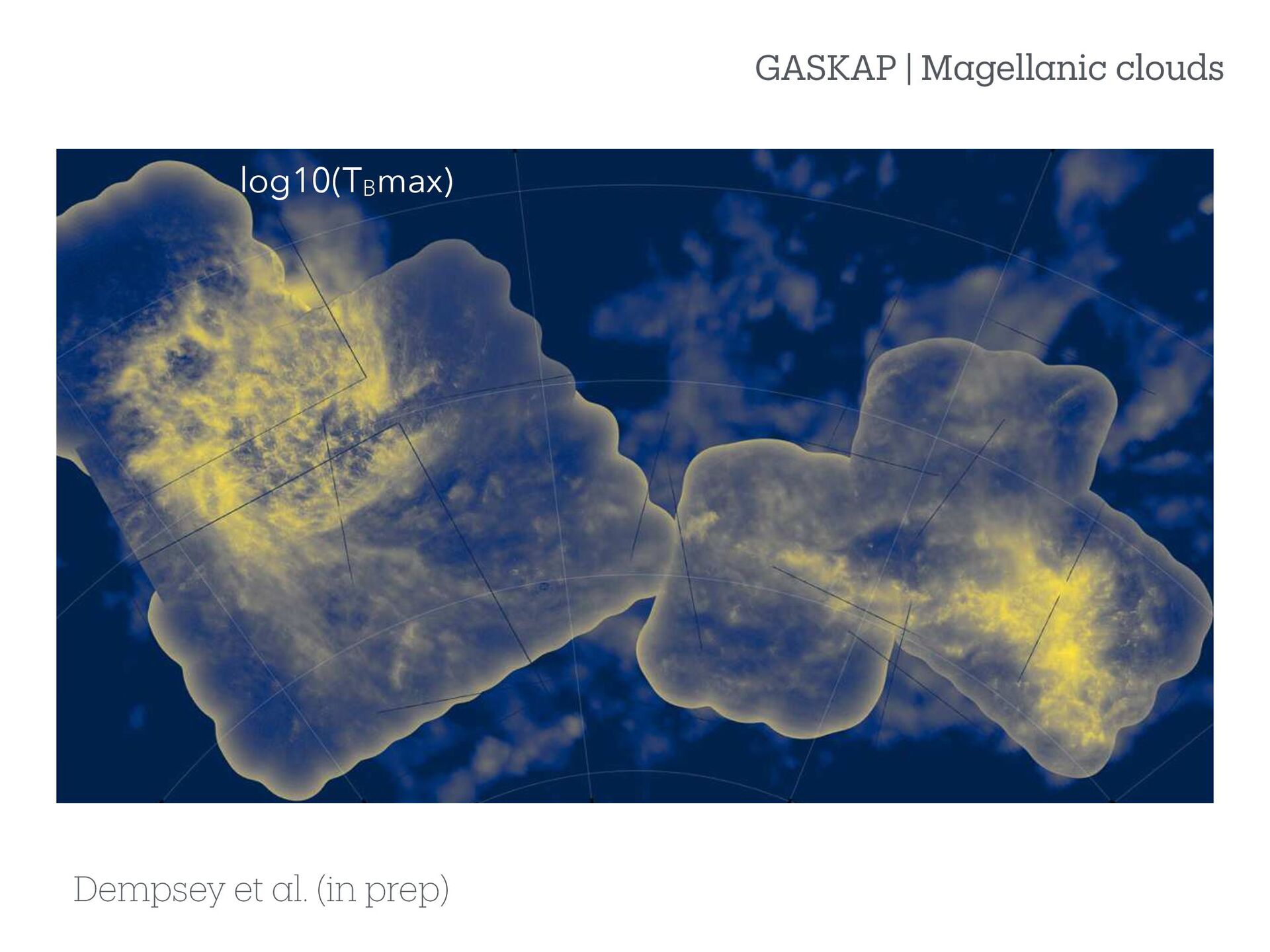
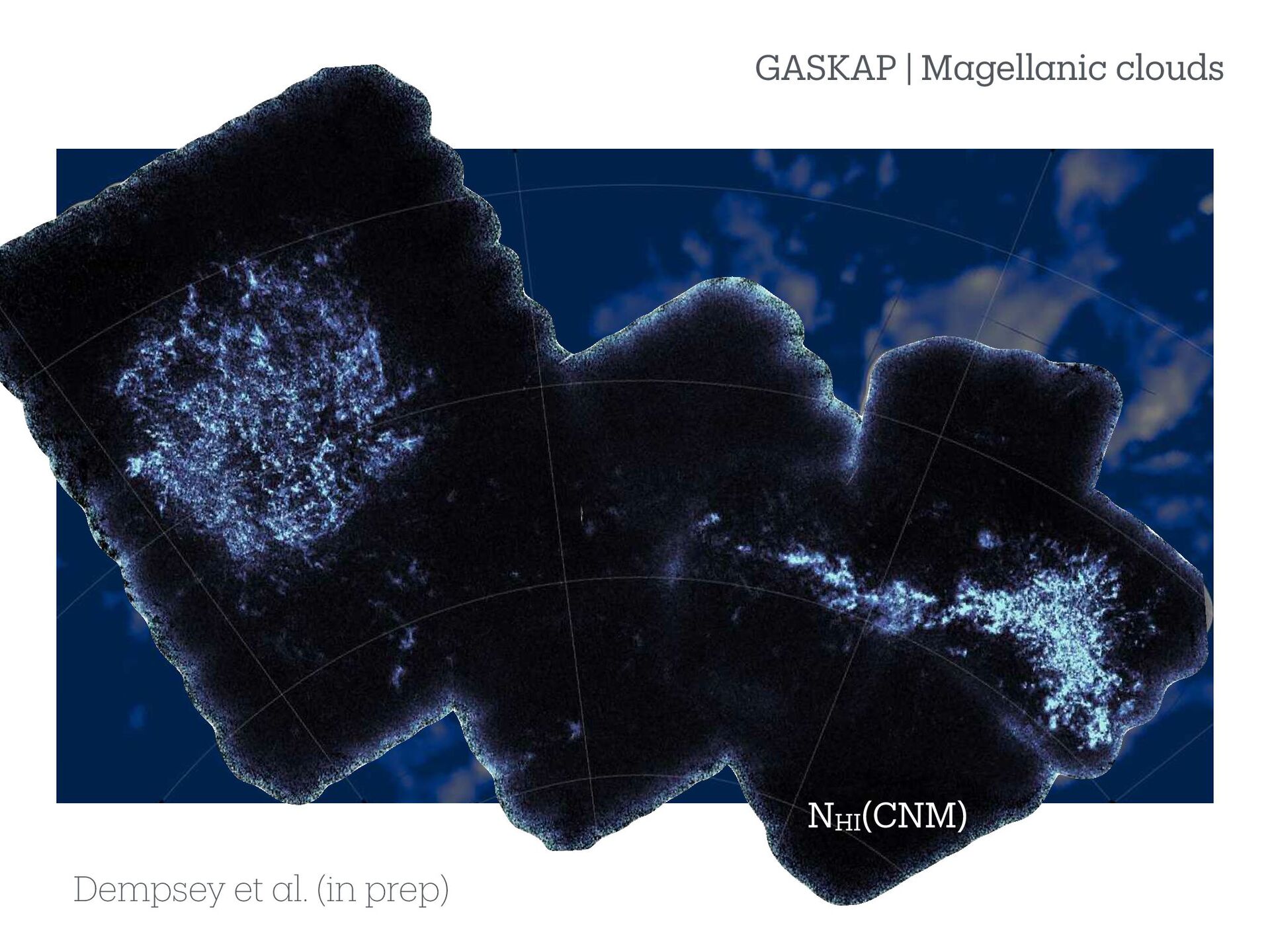
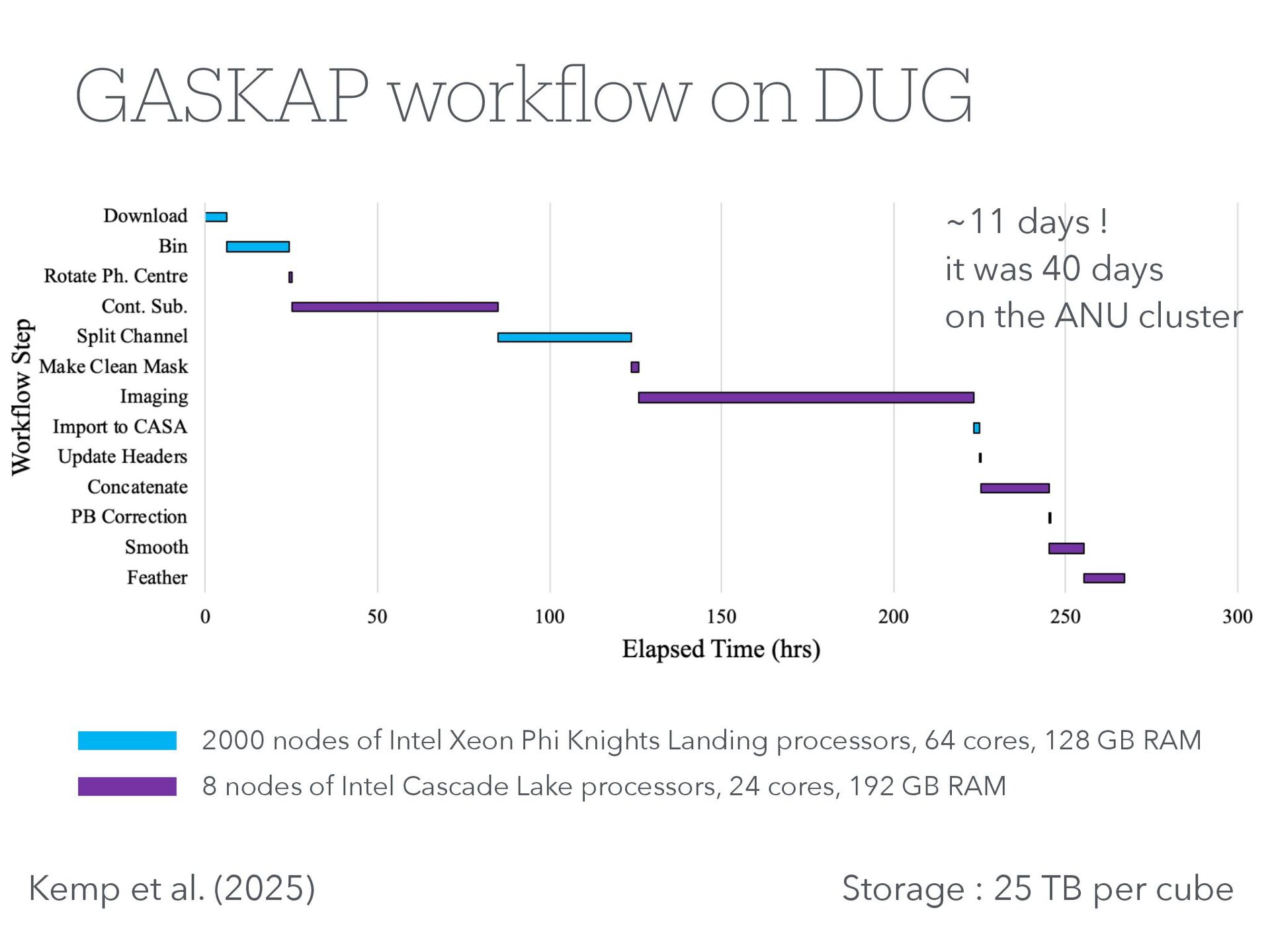
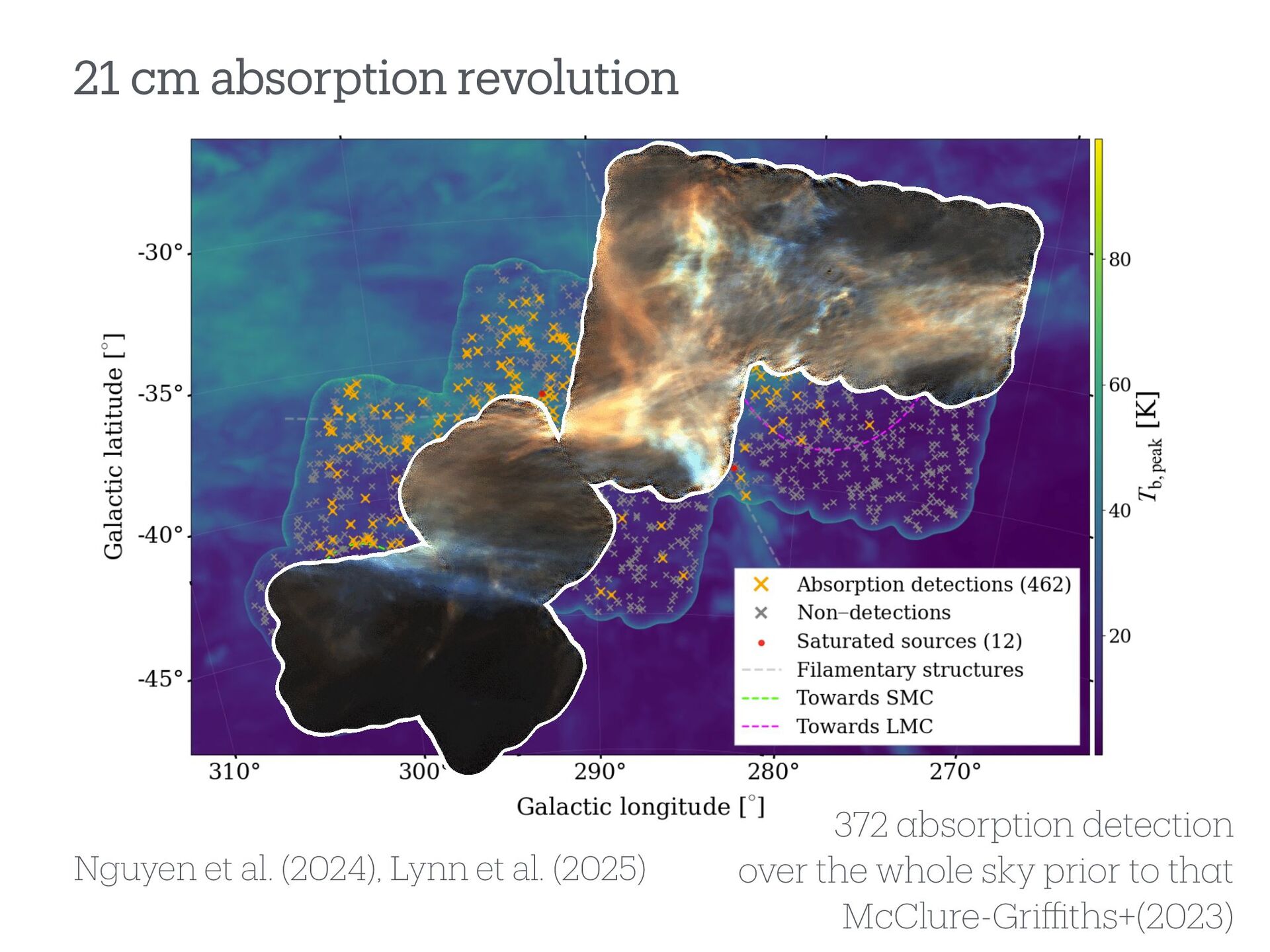
mapping of the MW and Magellanic system ¥ 2250 square degrees (5% of the whole sky) ¥ Magellanic Clouds : 150 deg2 ¥ Mag. Stream 1200 deg2 ¥ Gal Plane : 500 deg2 ¥ Galactic center : 400 deg2 ¥ Resolution : 20Ó, 0.2 km/s ¥ 4400 hours of telescope time ¥ Raw data ~ 3 PB ¥ Final product : ~40 Gb per Þeld (data cube ~ 2000x2000x100) ¥ 11 days of computing time to image one Þeld on commercial supercomputer in Australia ¥ Total project : 60 Þelds, 6 Tb (science ready)
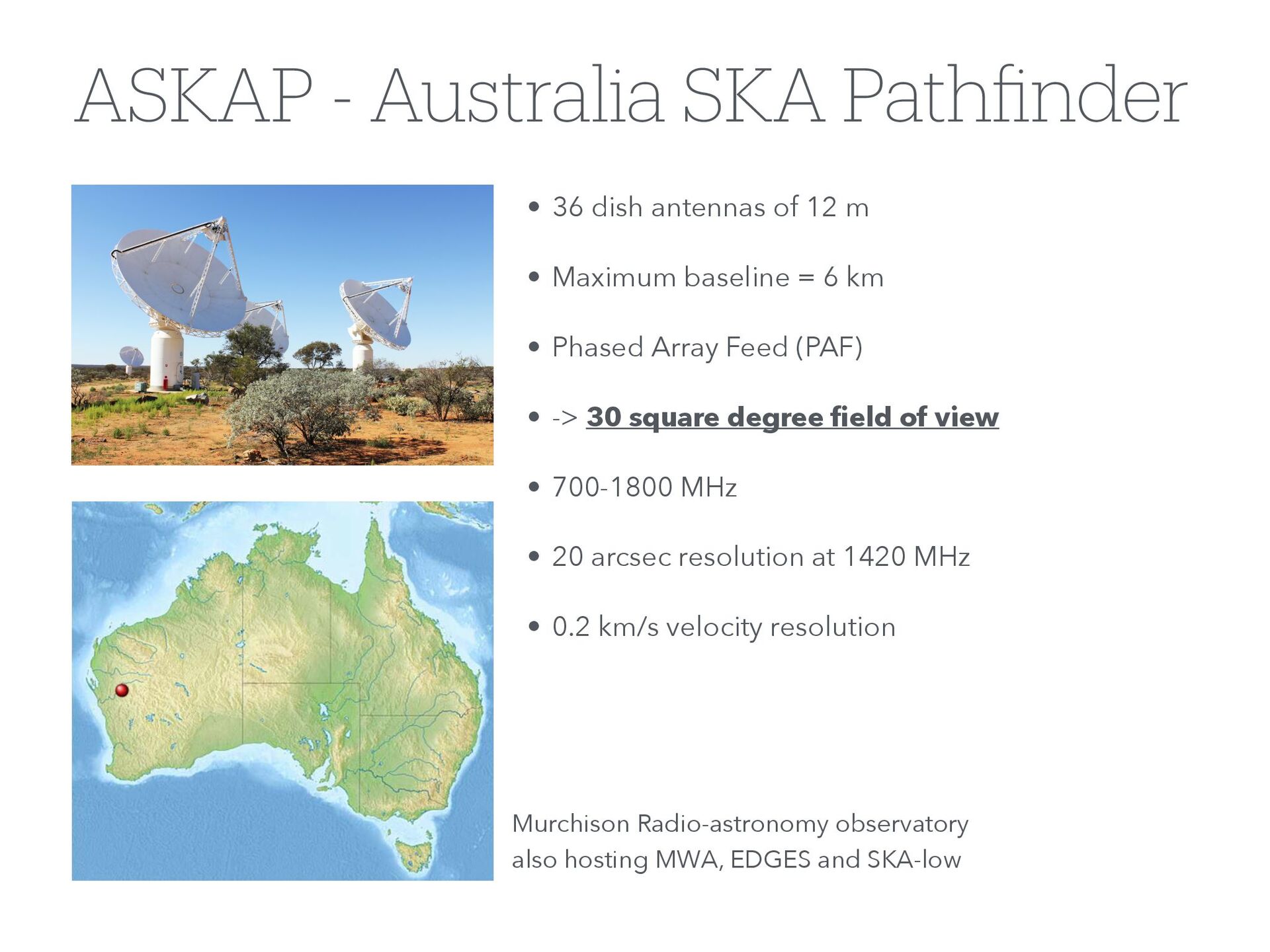
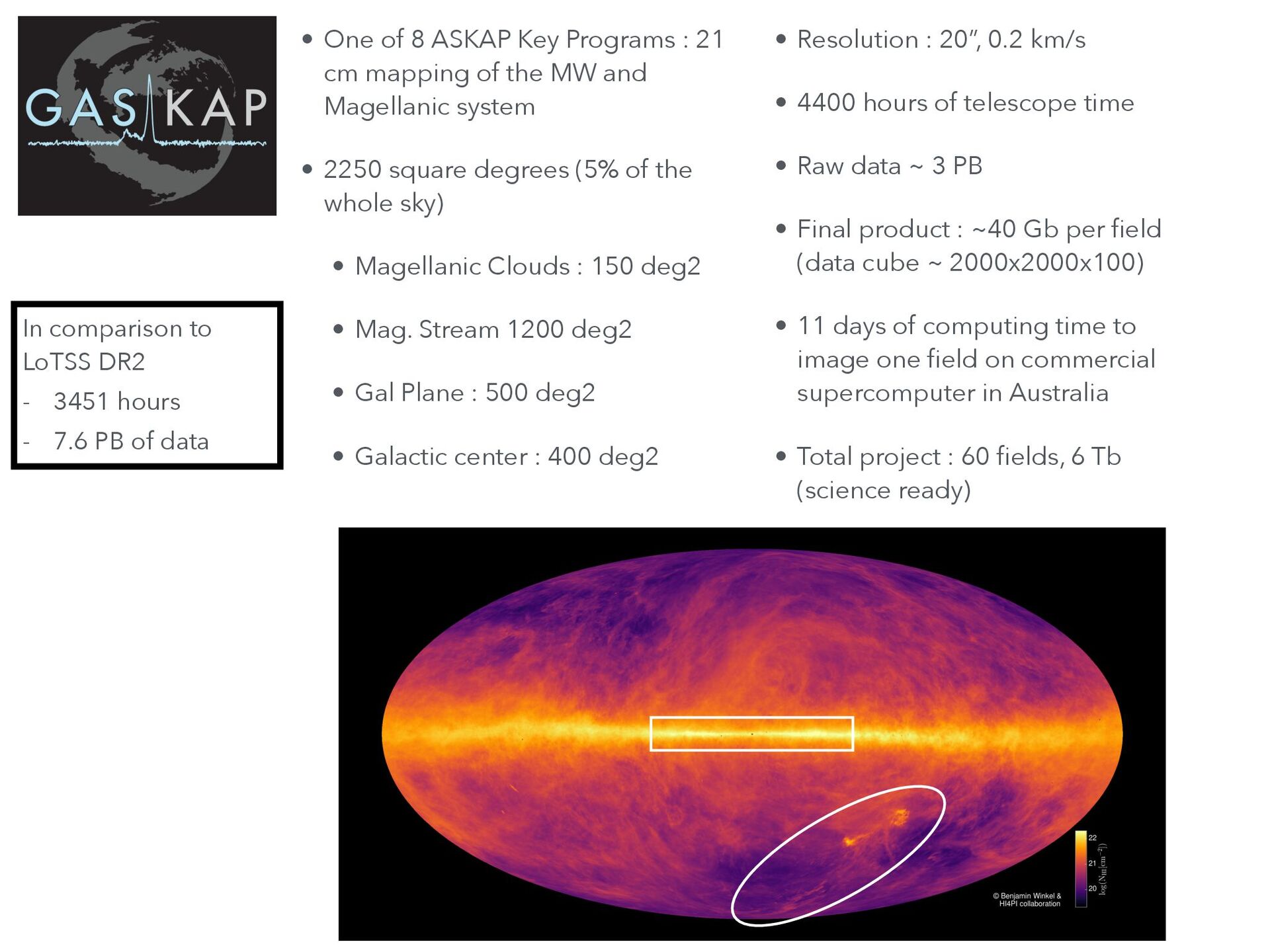
PB of data ¥ One of 8 ASKAP Key Programs : 21 cm mapping of the MW and Magellanic system ¥ 2250 square degrees (5% of the whole sky) ¥ Magellanic Clouds : 150 deg2 ¥ Mag. Stream 1200 deg2 ¥ Gal Plane : 500 deg2 ¥ Galactic center : 400 deg2 ¥ Resolution : 20Ó, 0.2 km/s ¥ 4400 hours of telescope time ¥ Raw data ~ 3 PB ¥ Final product : ~40 Gb per Þeld (data cube ~ 2000x2000x100) ¥ 11 days of computing time to image one Þeld on commercial supercomputer in Australia ¥ Total project : 60 Þelds, 6 Tb (science ready)
PB of data ¥ One of 8 ASKAP Key Programs : 21 cm mapping of the MW and Magellanic system ¥ 2250 square degrees (5% of the whole sky) ¥ Magellanic Clouds : 150 deg2 ¥ Mag. Stream 1200 deg2 ¥ Gal Plane : 500 deg2 ¥ Galactic center : 400 deg2 ¥ Resolution : 20Ó, 0.2 km/s ¥ 4400 hours of telescope time ¥ Raw data ~ 3 PB ¥ Final product : ~40 Gb per Þeld (data cube ~ 2000x2000x100) ¥ 11 days of computing time to image one Þeld on commercial supercomputer in Australia ¥ Total project : 60 Þelds, 6 Tb (science ready)
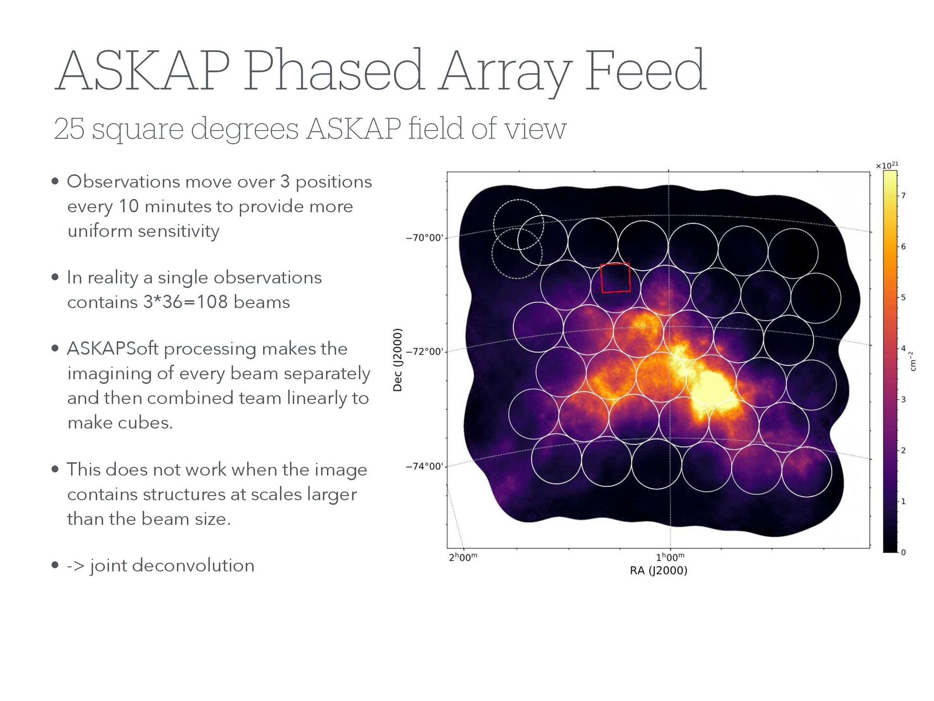
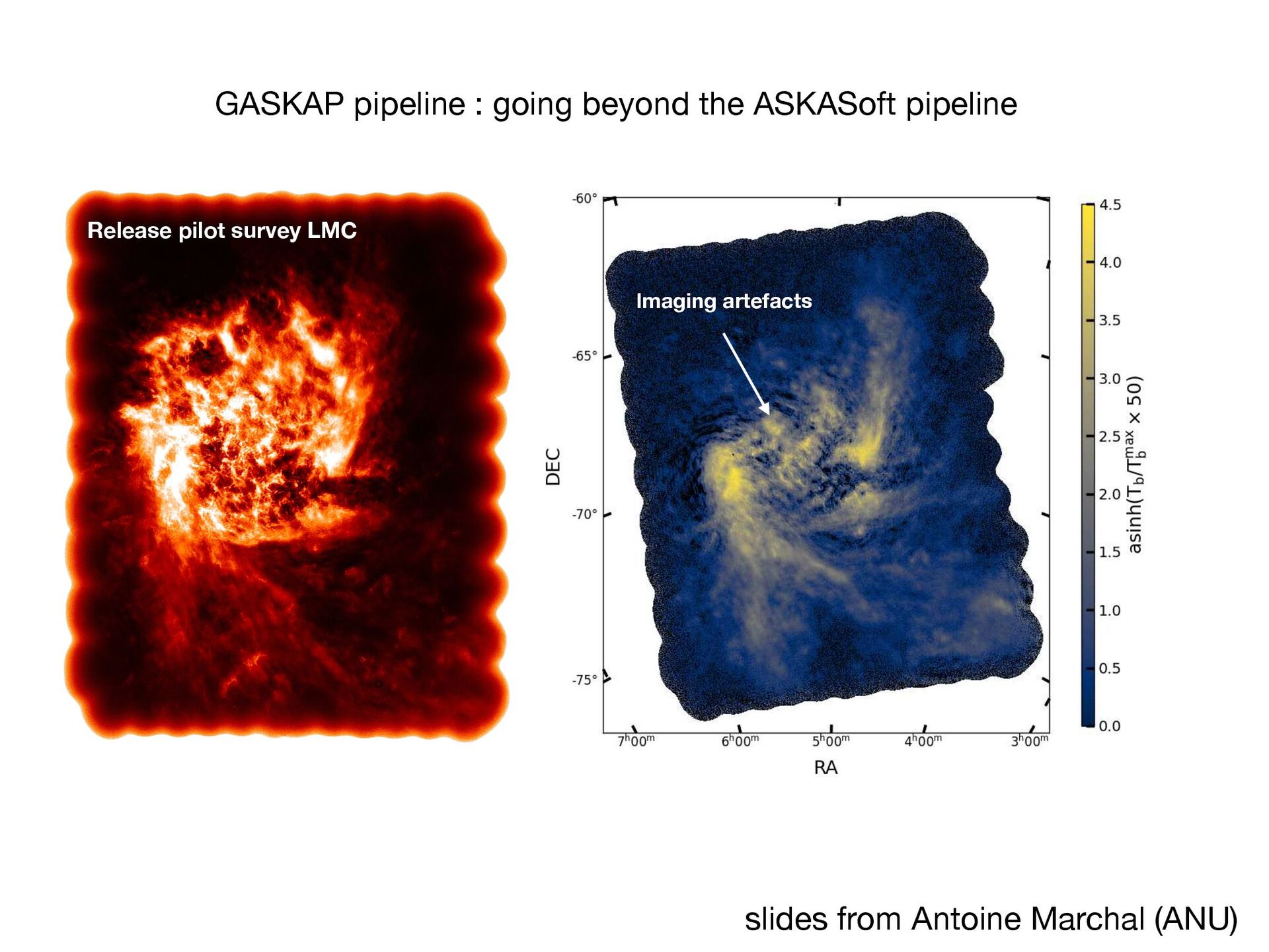
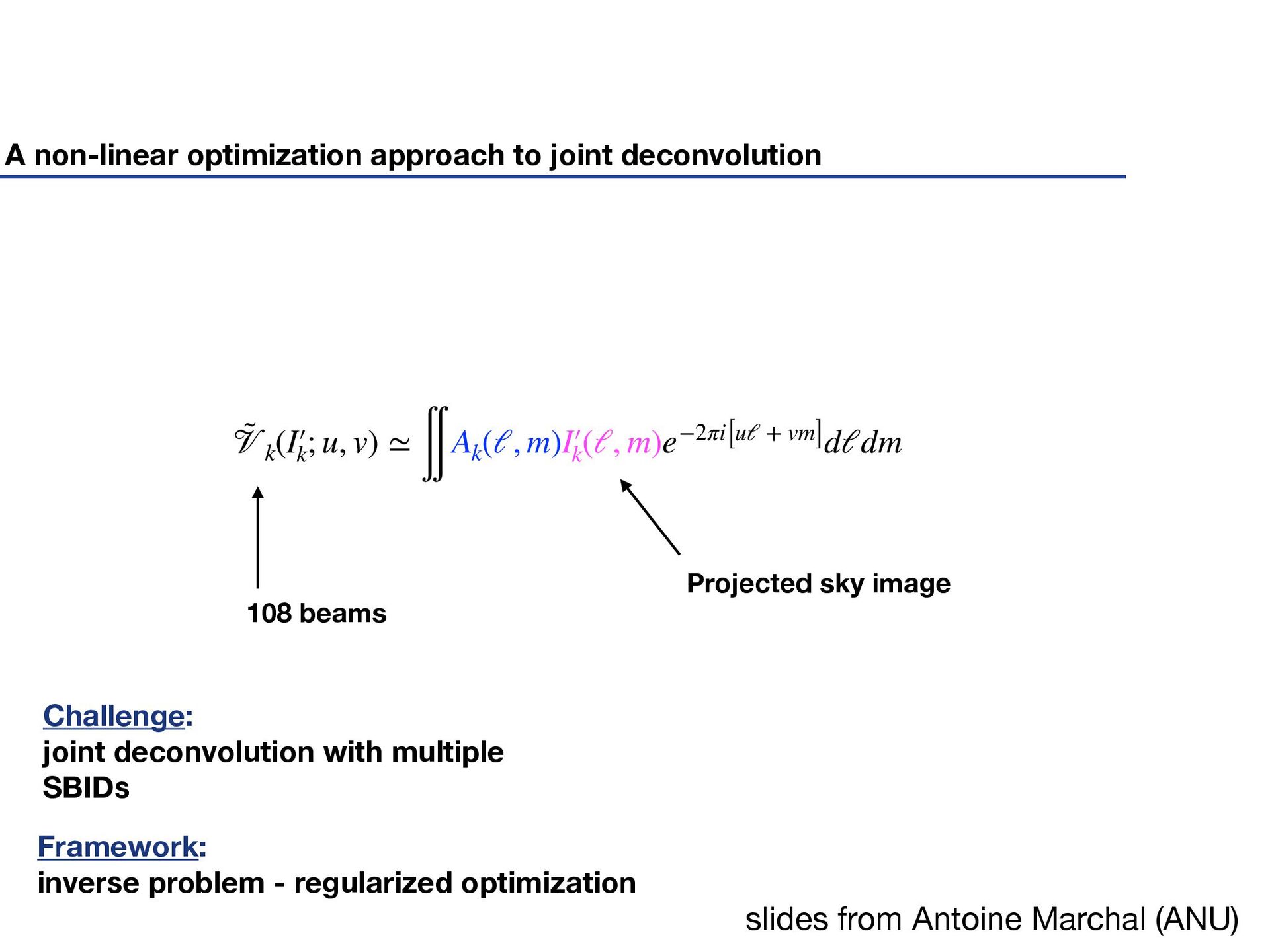
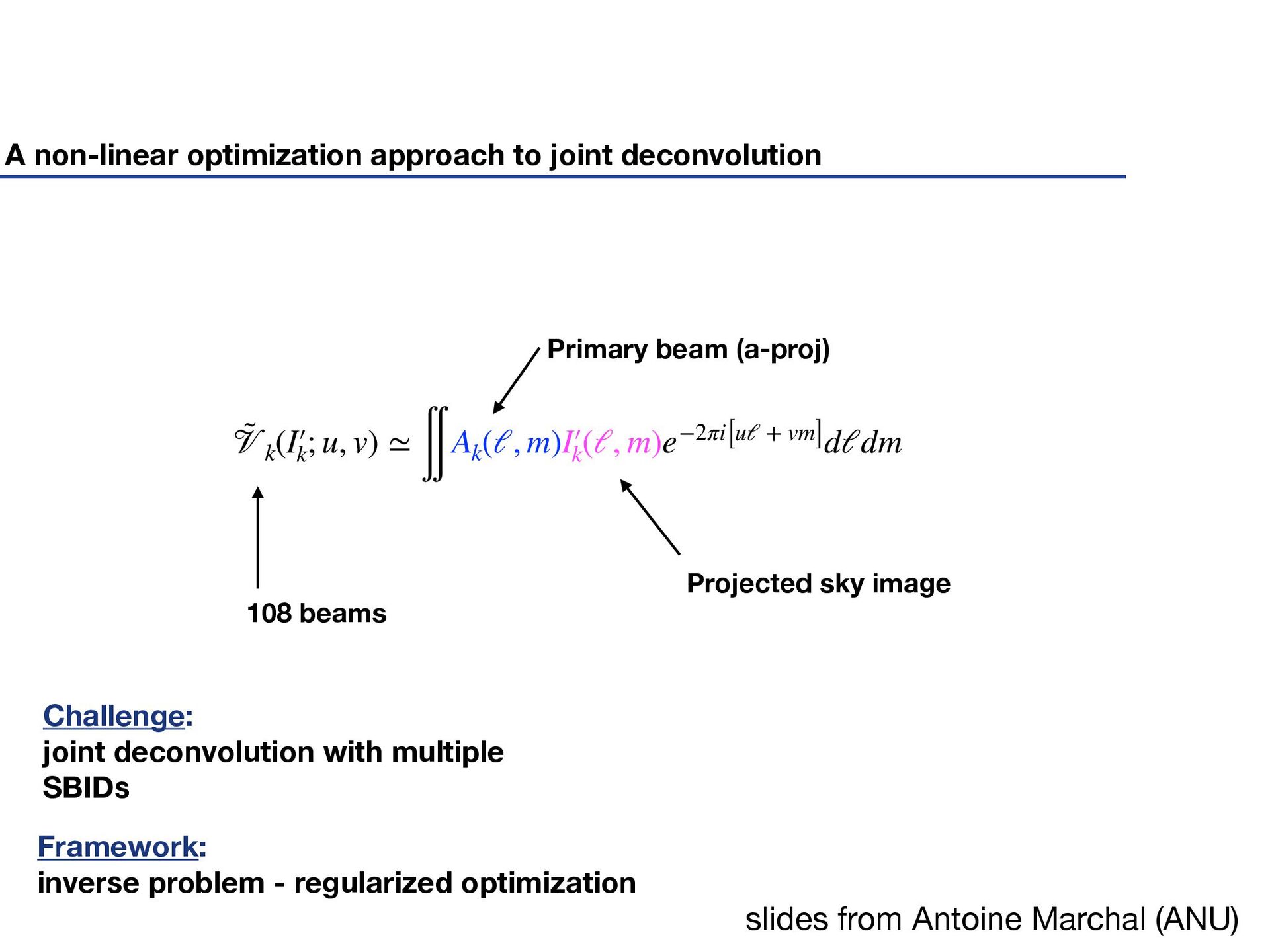
Feed ¥ Observations move over 3 positions every 10 minutes to provide more uniform sensitivity ¥ In reality a single observations contains 3*36=108 beams ¥ ASKAPSoft processing makes the imagining of every beam separately and then combined team linearly to make cubes. ¥ This does not work when the image contains structures at scales larger than the beam size. ¥ -> joint deconvolution
of Intel Xeon Phi Knights Landing processors, 64 cores, 128 GB RAM 8 nodes of Intel Cascade Lake processors, 24 cores, 192 GB RAM ~11 days ! it was 40 days on the ANU cluster Storage : 25 TB per cube
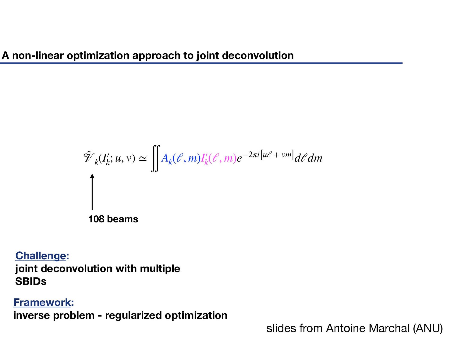
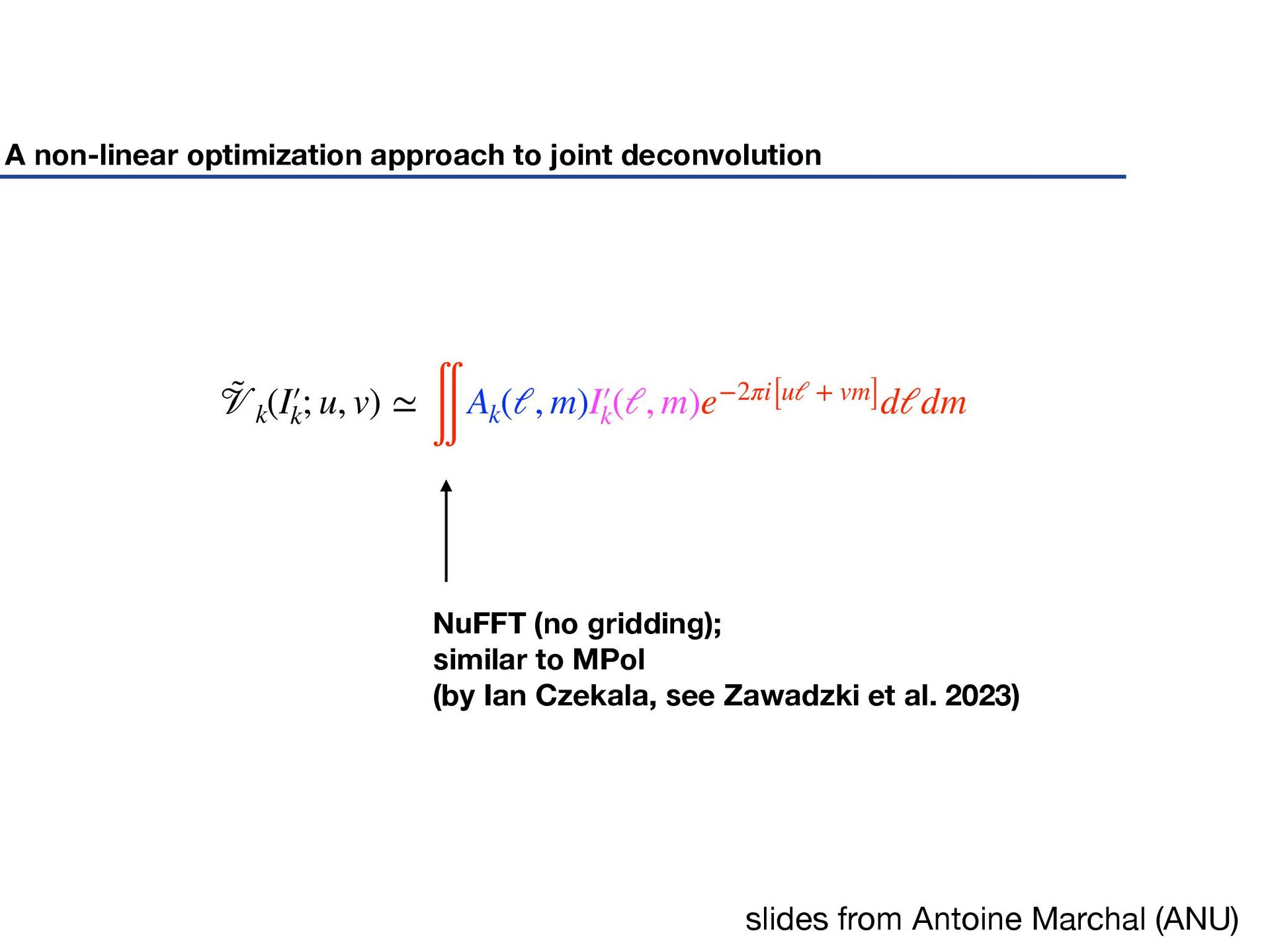
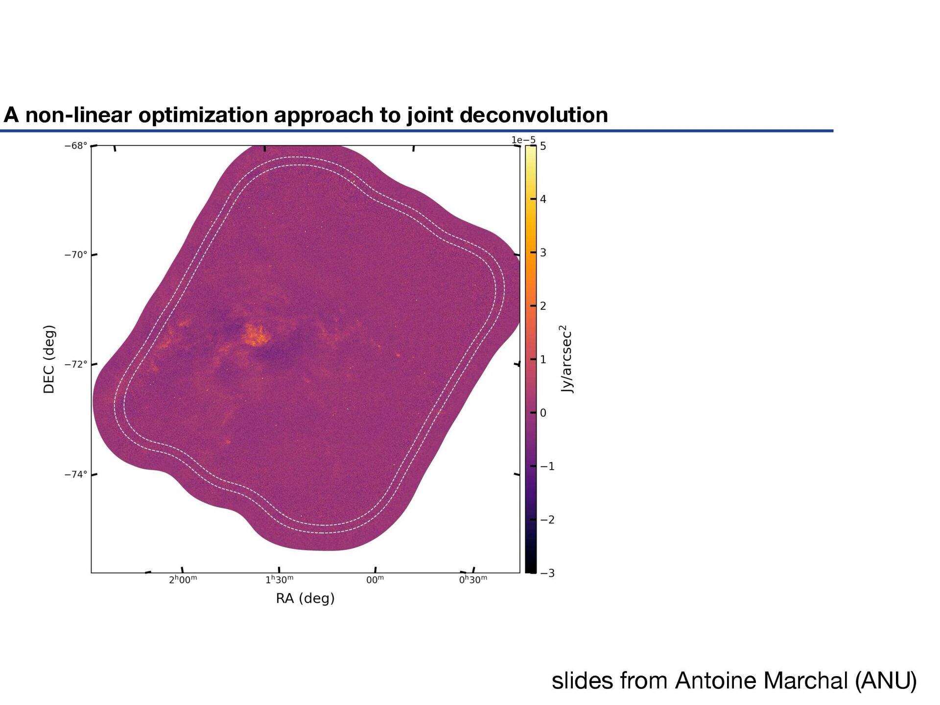
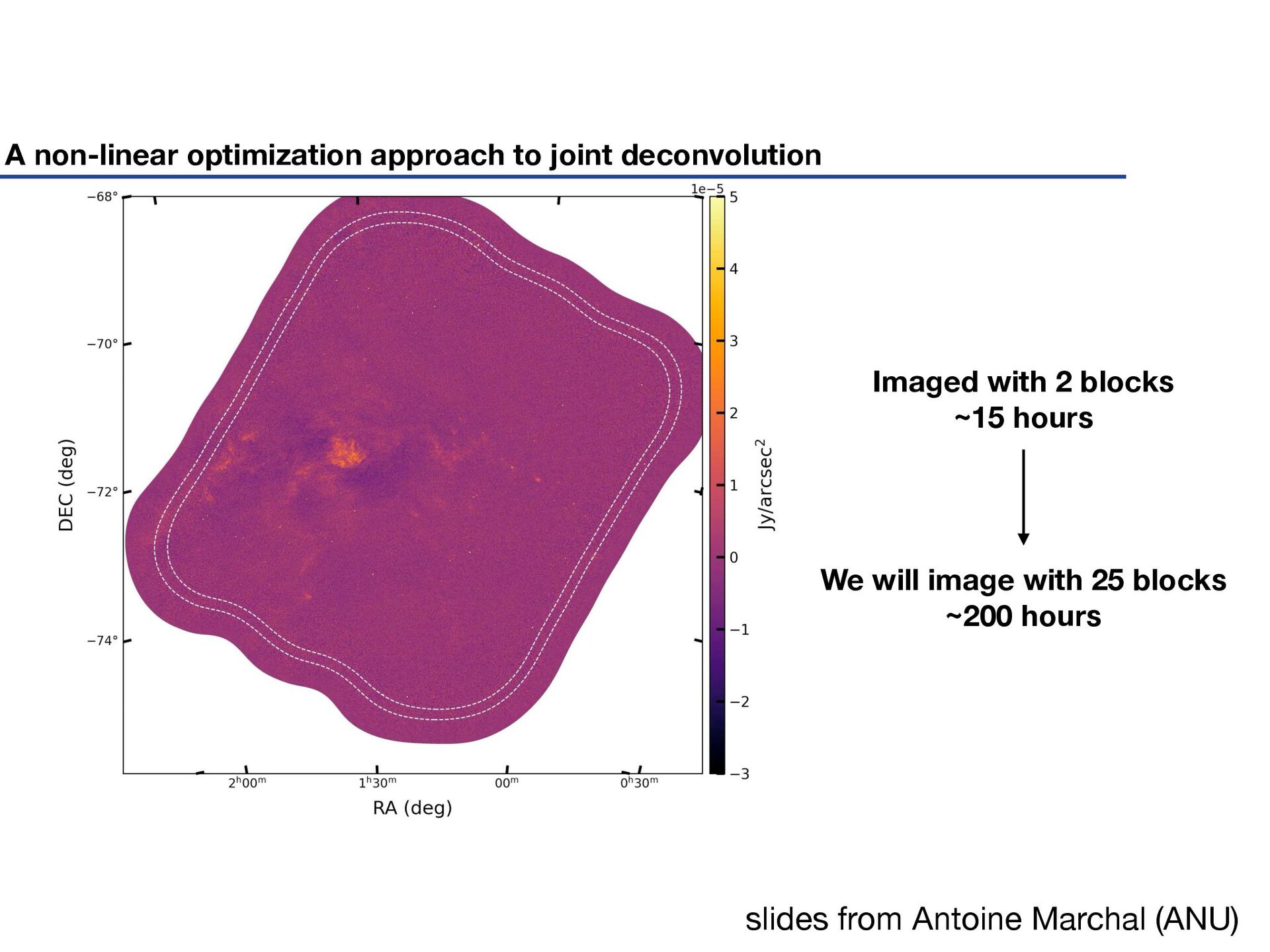
(ℓ, m)I′ k (ℓ, m)e−2πi[uℓ + vm]dℓdm Framework: inverse problem - regularized optimization 108 beams Challenge: joint deconvolution with multiple SBIDs A non-linear optimization approach to joint deconvolution slides from Antoine Marchal (ANU)
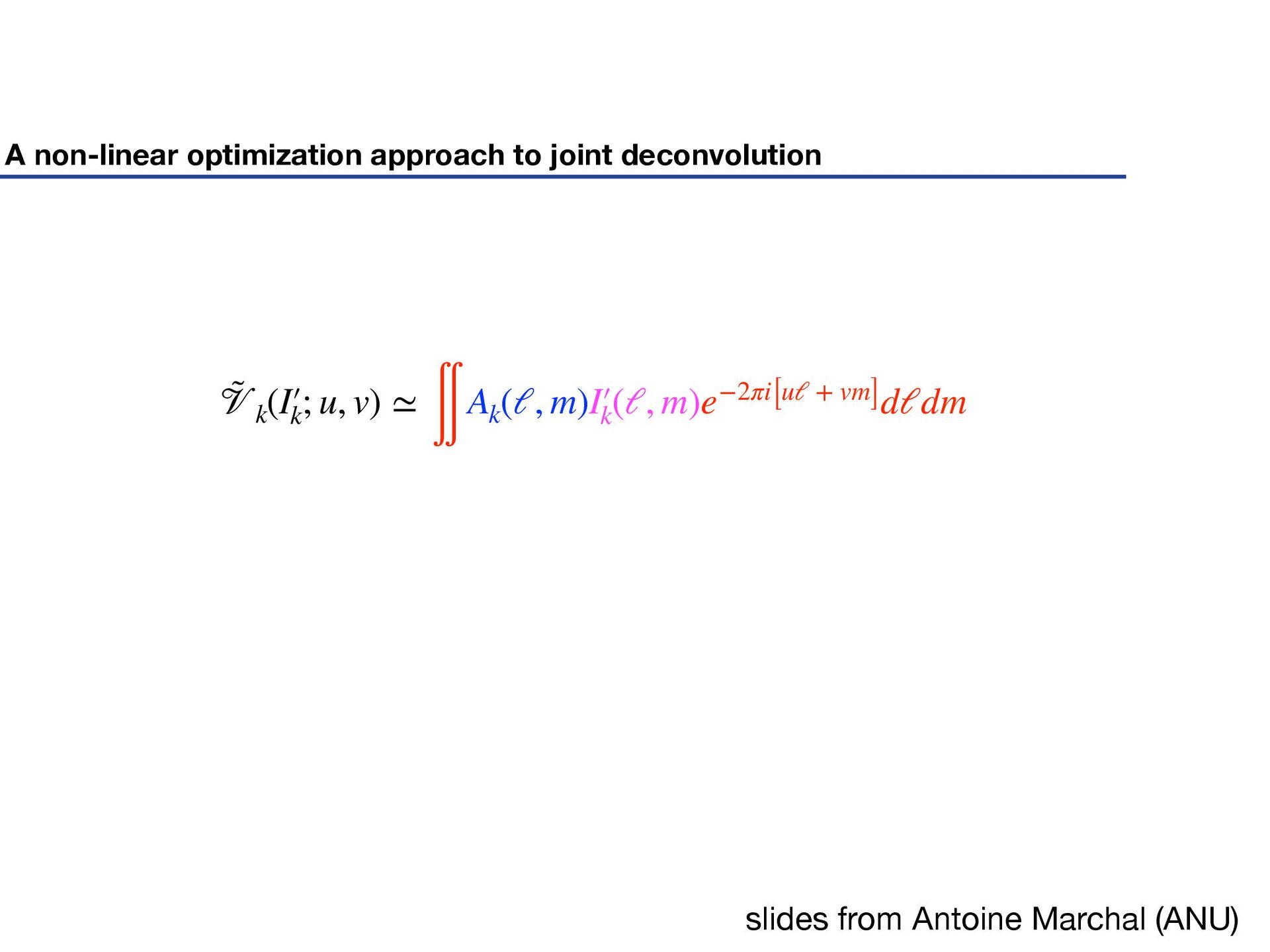
(ℓ, m)I′ k (ℓ, m)e−2πi[uℓ + vm]dℓdm NuFFT (no gridding); similar to MPol (by Ian Czekala, see Zawadzki et al. 2023) A non-linear optimization approach to joint deconvolution slides from Antoine Marchal (ANU)
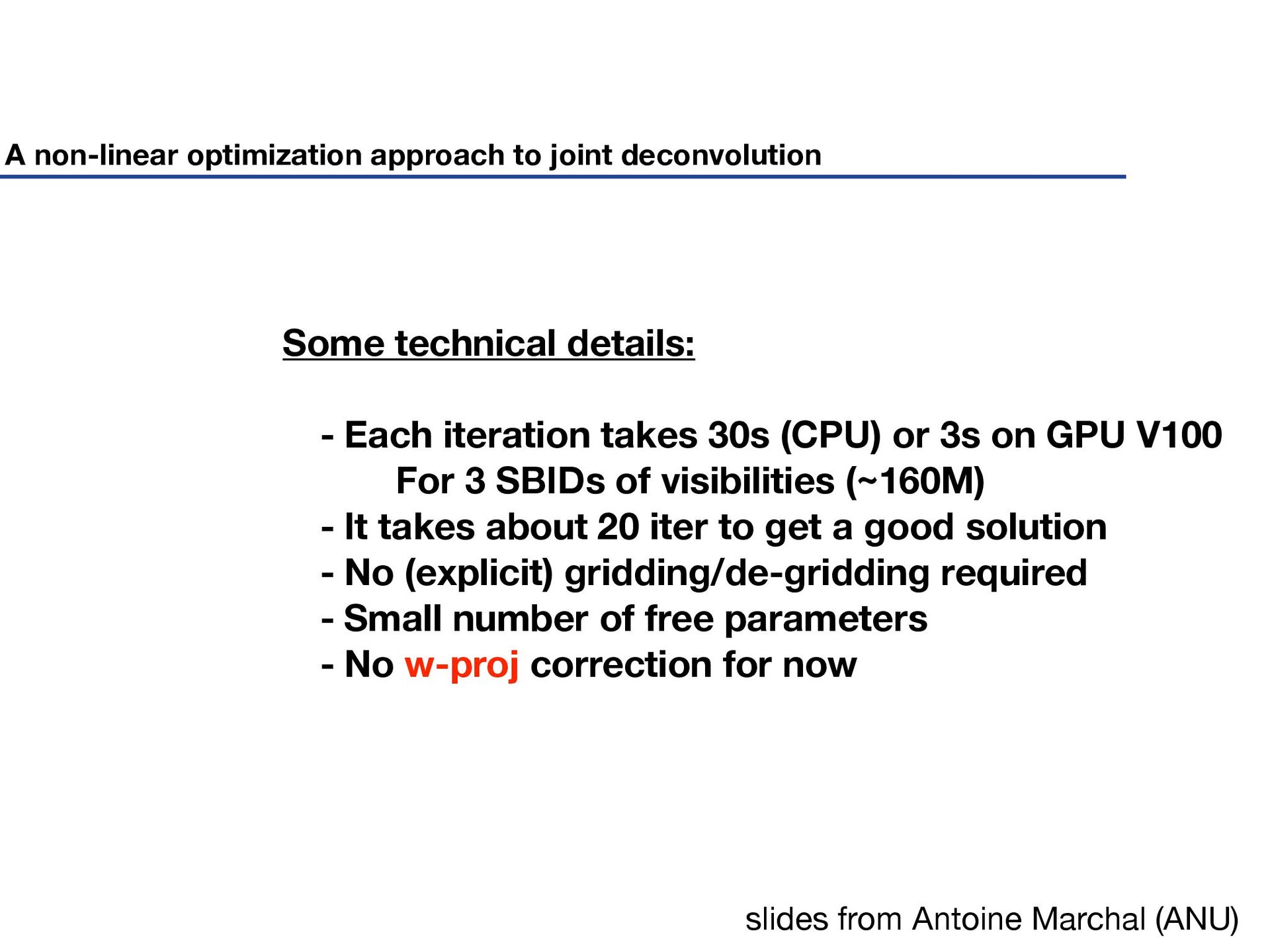
3s on GPU V100 For 3 SBIDs of visibilities (~160M) - It takes about 20 iter to get a good solution - No (explicit) gridding/de-gridding required - Small number of free parameters - No w-proj correction for now A non-linear optimization approach to joint deconvolution slides from Antoine Marchal (ANU)
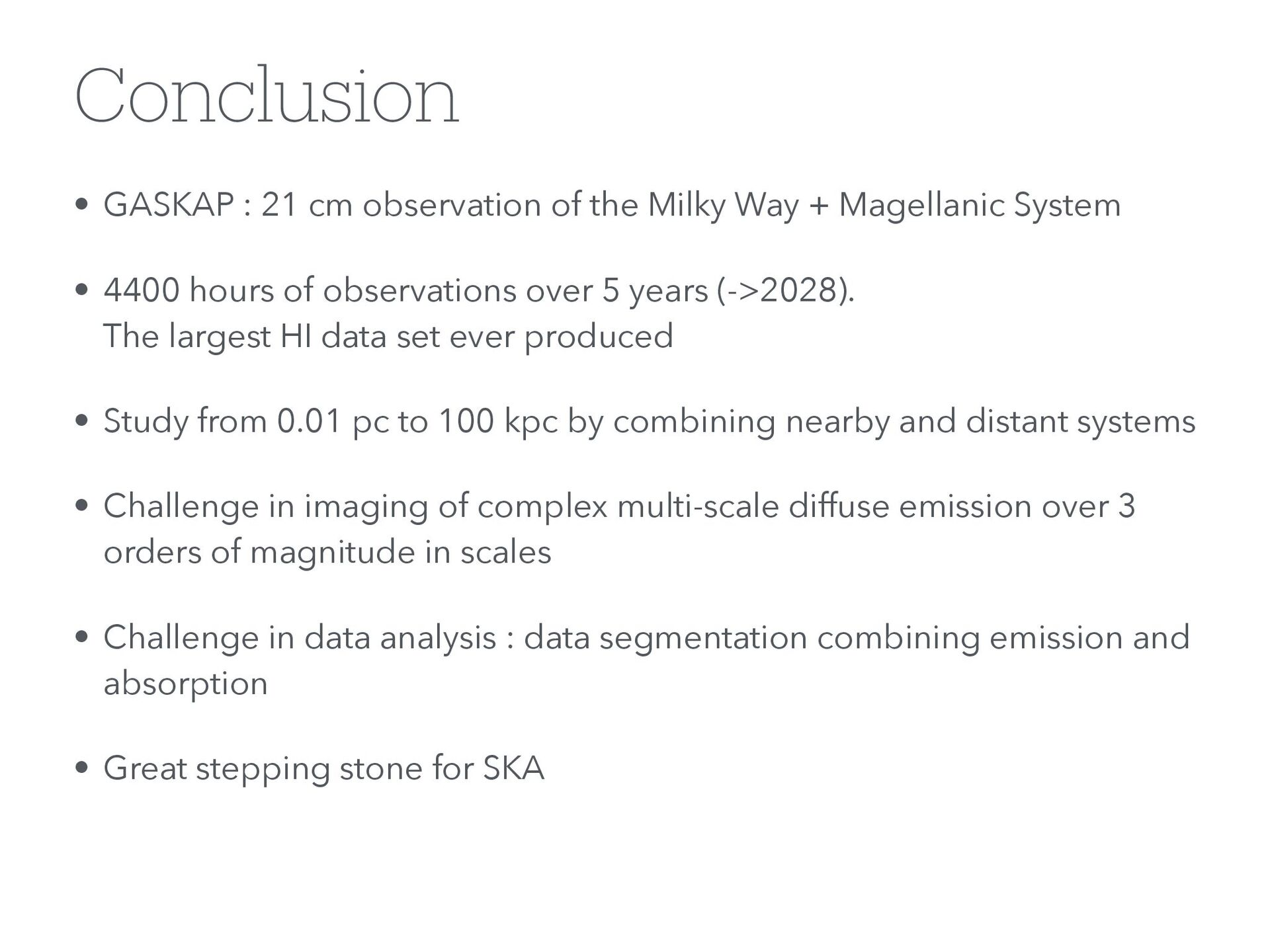
Way + Magellanic System ¥ 4400 hours of observations over 5 years (->2028). The largest HI data set ever produced ¥ Study from 0.01 pc to 100 kpc by combining nearby and distant systems ¥ Challenge in imaging of complex multi-scale diffuse emission over 3 orders of magnitude in scales ¥ Challenge in data analysis : data segmentation combining emission and absorption ¥ Great stepping stone for SKA
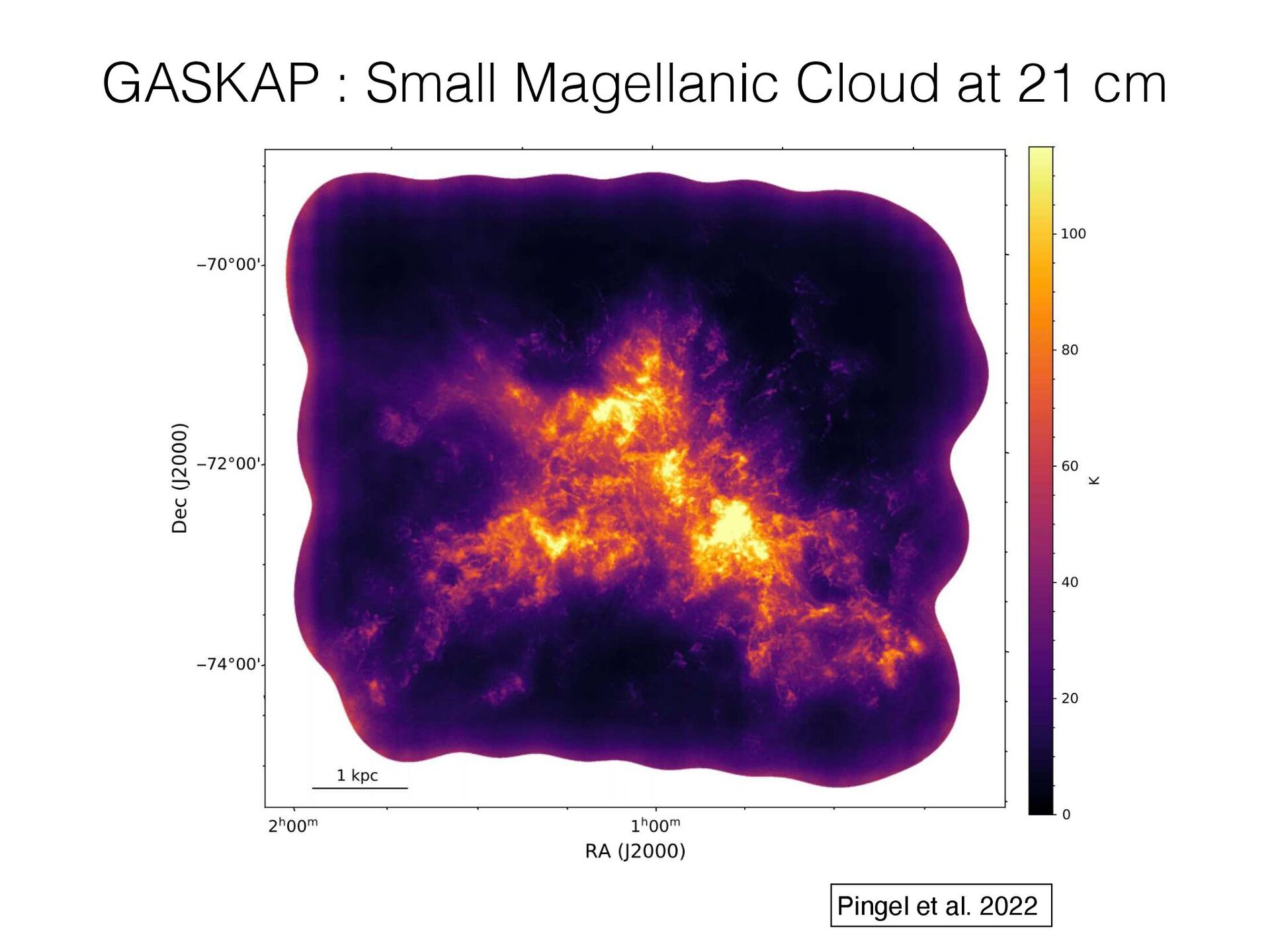
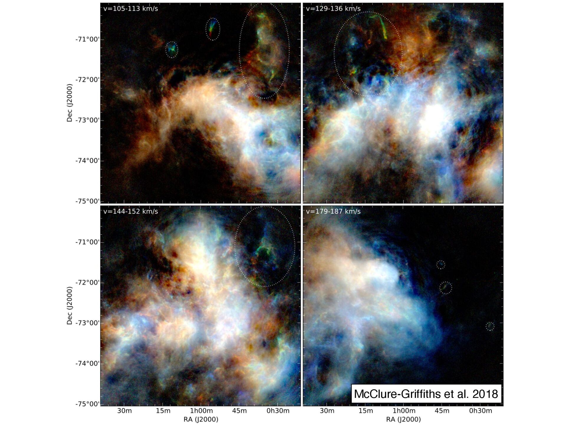
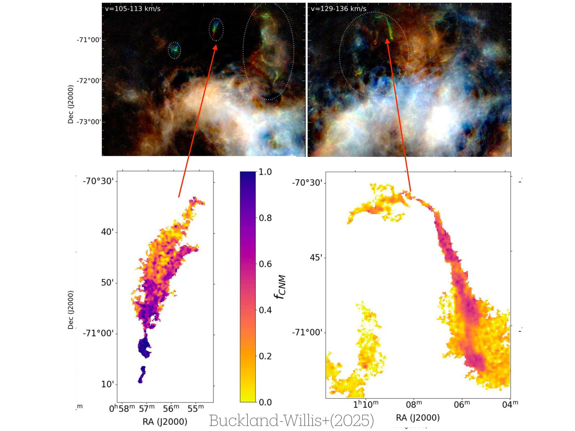
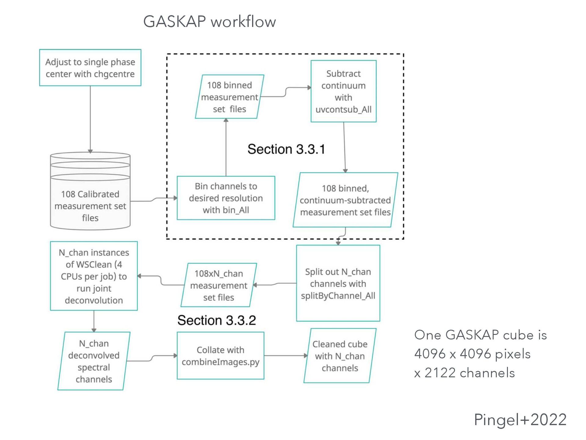
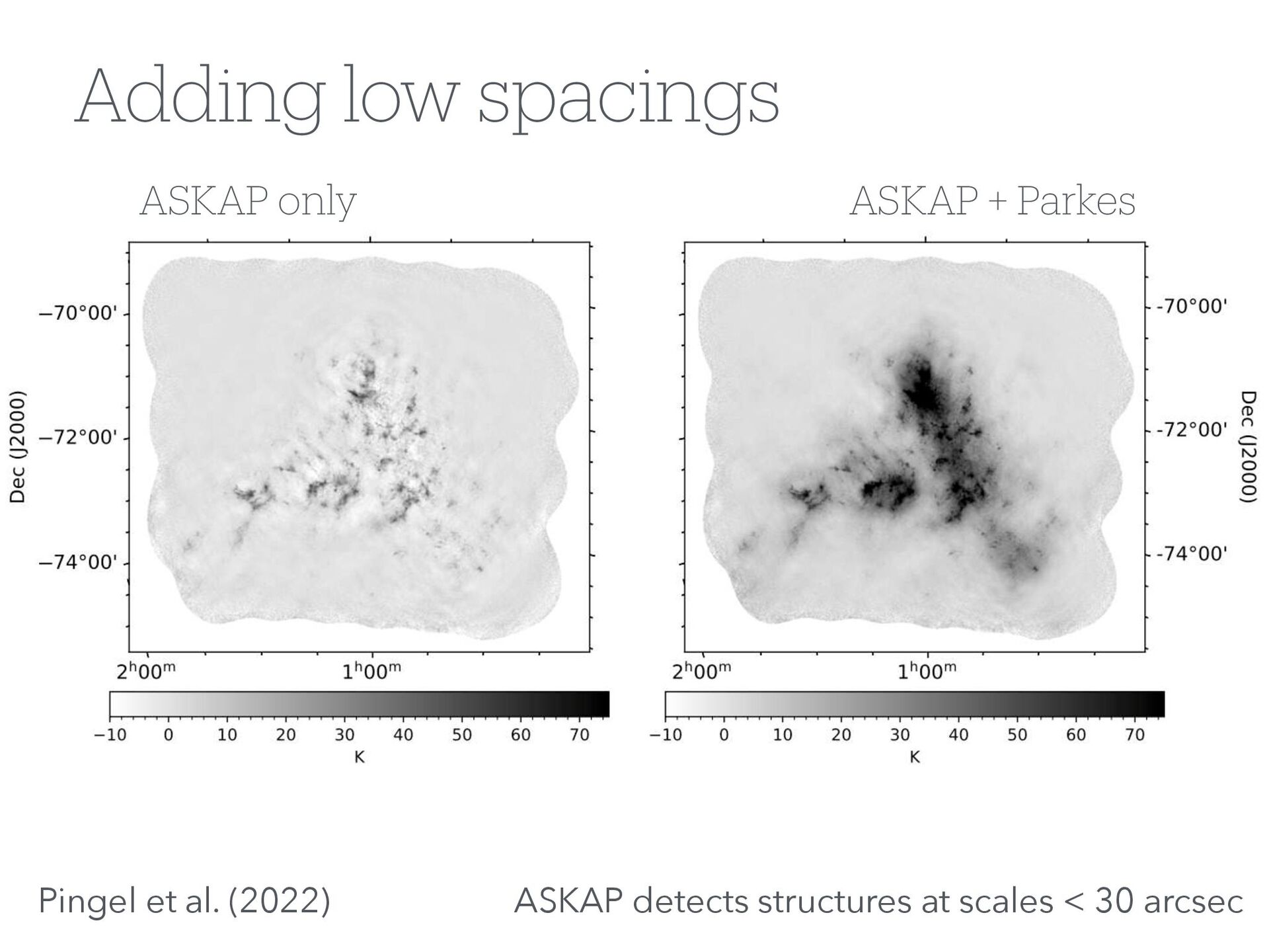
survey data using a commercial supercomputer ¥ Pingel et al. (2022), GASKAP-HI PILOT survey science 1; ASKAP Zoom observations of HI emission in the Smal Magellanic Cloud ¥ Marchal et al. (2019), ROHSA; Regularized Optmiziation for Hyper- Spectral Analysis - Application to phase separation of 21 cm data ¥ McClure-GrifÞths et al. (2019), Cold gas outßows from the Small Magellanic Cloud traced with ASKAP
![TB[v] for 16 adjacent lines of sight Integrated emission of](https://files.speakerdeck.com/presentations/28ffbbb956894778899844de1f20530f/slide_19.jpg)
![TB[v] for 16 adjacent lines of sight Integrated emission of](https://files.speakerdeck.com/presentations/28ffbbb956894778899844de1f20530f/slide_20.jpg)