ThermoGS (ECCV2026)解説 — 4D Gaussian Splatting × Thermodynamics CVと物理の統合モデルとして

第68回 コンピュータビジョン勉強会＠関東(https://kantocv.connpass.com/event/407846/)にて解説補助用に作成しました。
解説スライドはClaudeを使用し作成しました。
解説動画はClaudeにて解説スライドを基に生成しました。
元論文を参照し作成しましたが、誤植等が含まれる可能性があるため、詳細は元論文をご確認ください。
ThermoGS: Decoupling Physical Surface
Attributes for Spatio-Temporal Thermal Field
Emulation via 4D Gaussian Splatting
(https://media.eventhosts.cc/Conferences/ECCV2026/pdfs/3713.pdf)

Transcript

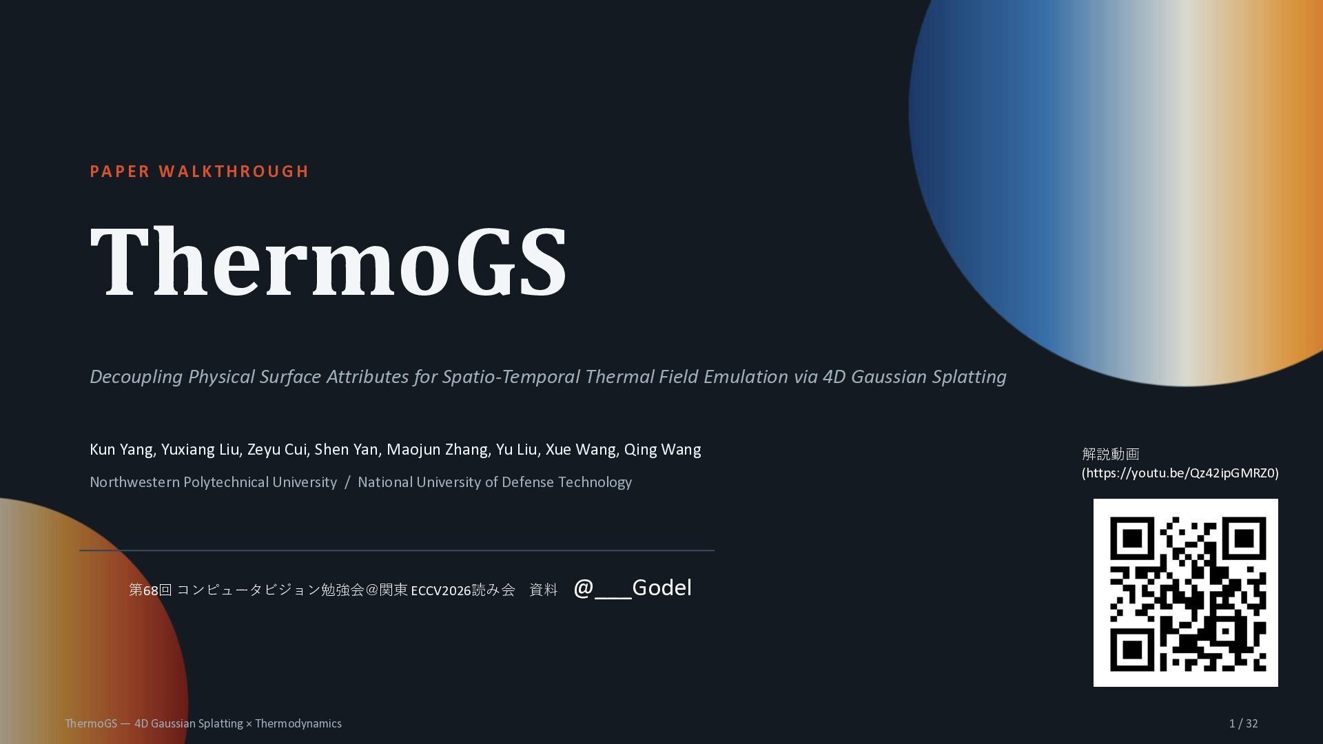
1. PAPER WALKTHROUGH ThermoGS Decoupling Physical Surface Attributes for Spatio-Temporal Thermal Field Emulation via 4D Gaussian Splatting Kun Yang, Yuxiang Liu, Zeyu Cui, Shen Yan, Maojun Zhang, Yu Liu, Xue Wang, Qing Wang Northwestern Polytechnical University / National University of Defense Technology 第68回 コンピュータビジョン勉強会＠関東 ECCV2026読み会 資料 ThermoGS — 4D Gaussian Splatting × Thermodynamics 解説動画 (https://youtu.be/Qz42ipGMRZ0) @___Godel 1 / 32
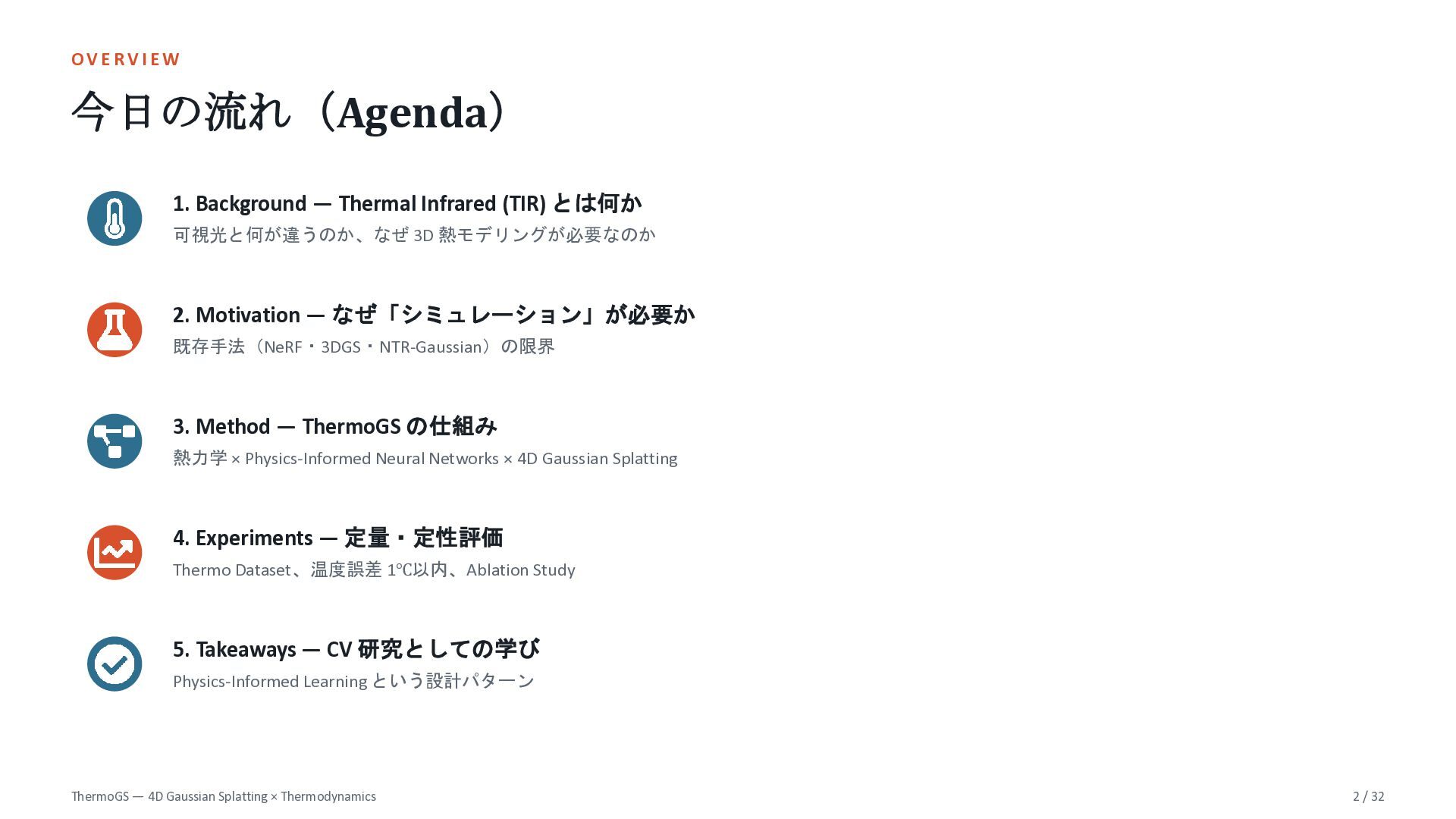
2. OVERVIEW 今日の流れ（Agenda） 1. Background — Thermal Infrared (TIR) とは何か 可視光と何が違うのか、なぜ 3D 熱モデリングが必要なのか 2. Motivation — なぜ「シミュレーション」が必要か 既存手法（NeRF・3DGS・NTR-Gaussian）の限界 3. Method — ThermoGS の仕組み 熱力学 × Physics-Informed Neural Networks × 4D Gaussian Splatting 4. Experiments — 定量・定性評価 Thermo Dataset、温度誤差 1℃以内、Ablation Study 5. Takeaways — CV 研究としての学び Physics-Informed Learning という設計パターン ThermoGS — 4D Gaussian Splatting × Thermodynamics 2 / 32
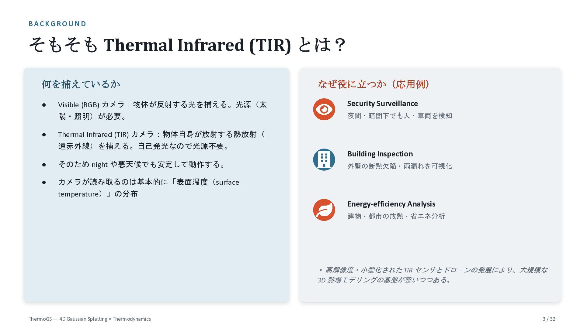
3. BACKGROUND そもそも Thermal Infrared (TIR) とは？ 何を捕えているか • • Visible (RGB) カメラ：物体が反射する光を捕える。光源（太 陽・照明）が必要。 なぜ役に立つか（応用例） Security Surveillance 夜間・暗闇下でも人・車両を検知 Thermal Infrared (TIR) カメラ：物体自身が放射する熱放射（ 遠赤外線）を捕える。自己発光なので光源不要。 Building Inspection • そのため night や悪天候でも安定して動作する。 • カメラが読み取るのは基本的に「表面温度（surface 外壁の断熱欠陥・雨漏れを可視化 temperature）」の分布 Energy-efficiency Analysis 建物・都市の放熱・省エネ分析 ▸ 高解像度・小型化された TIR センサとドローンの発展により、大規模な 3D 熱場モデリングの基盤が整いつつある。 ThermoGS — 4D Gaussian Splatting × Thermodynamics 3 / 32
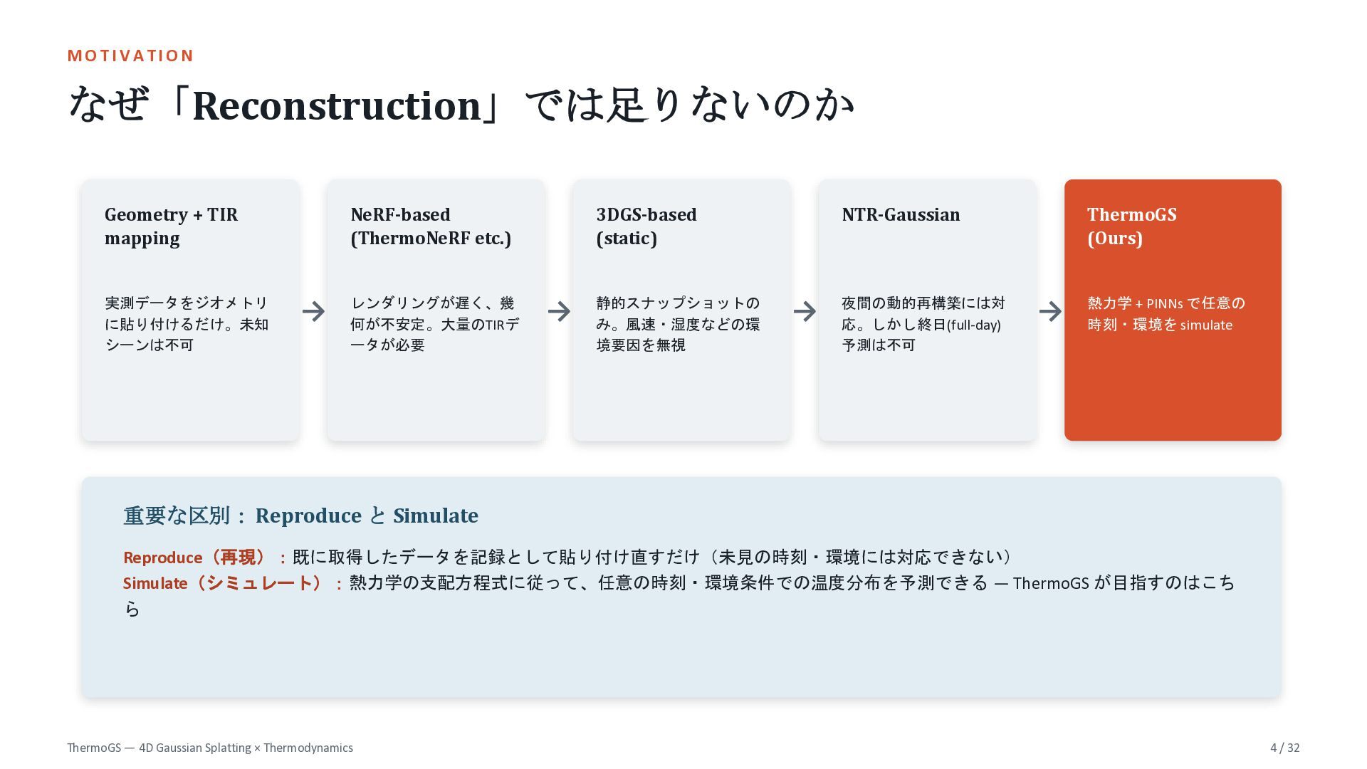
4. MOTIVATION なぜ「Reconstruction」では足りないのか Geometry + TIR mapping 実測データをジオメトリ に貼り付けるだけ。未知 シーンは不可 NeRF-based (ThermoNeRF etc.) → レンダリングが遅く、幾 何が不安定。大量のTIRデ ータが必要 3DGS-based (static) → 静的スナップショットの み。風速・湿度などの環 境要因を無視 NTR-Gaussian → 夜間の動的再構築には対 応。しかし終日(full-day) 予測は不可 ThermoGS (Ours) → 熱力学 + PINNs で任意の 時刻・環境を simulate 重要な区別： Reproduce と Simulate Reproduce（再現）：既に取得したデータを記録として貼り付け直すだけ（未見の時刻・環境には対応できない） Simulate（シミュレート）：熱力学の支配方程式に従って、任意の時刻・環境条件での温度分布を予測できる — ThermoGS が目指すのはこち ら ThermoGS — 4D Gaussian Splatting × Thermodynamics 4 / 32
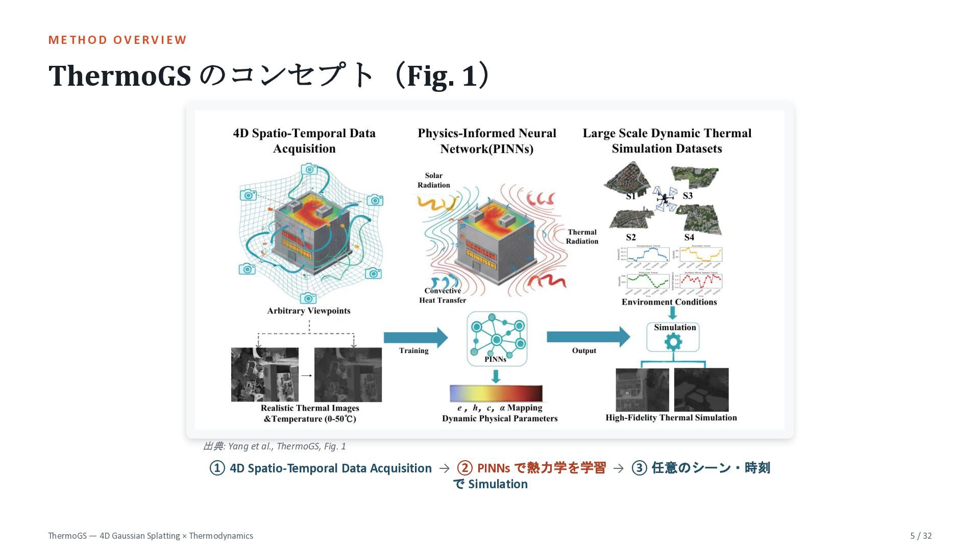
5. METHOD OVERVIEW ThermoGS のコンセプト（Fig. 1） 出典: Yang et al., ThermoGS, Fig. 1 ① 4D Spatio-Temporal Data Acquisition → ② PINNs で熱力学を学習 → ③ 任意のシーン・時刻 で Simulation ThermoGS — 4D Gaussian Splatting × Thermodynamics 5 / 32
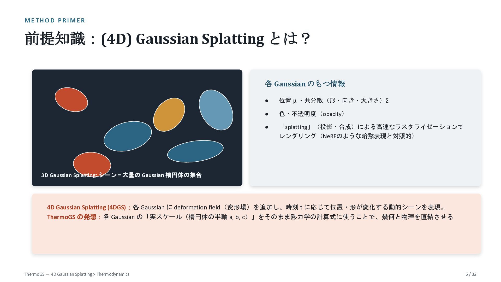
6. METHOD PRIMER 前提知識：(4D) Gaussian Splatting とは？ 各 Gaussian のもつ情報 • 位置 μ ・共分散（形・向き・大きさ）Σ • 色・不透明度（opacity） • 「splatting」（投影・合成）による高速なラスタライゼーションで レンダリング（NeRFのような暗黙表現と対照的） 3D Gaussian Splatting: シーン = 大量の Gaussian 楕円体の集合 4D Gaussian Splatting (4DGS)：各 Gaussian に deformation field（変形場）を追加し、時刻 t に応じて位置・形が変化する動的シーンを表現。 ThermoGS の発想：各 Gaussian の「実スケール（楕円体の半軸 a, b, c）」をそのまま熱力学の計算式に使うことで、幾何と物理を直結させる ThermoGS — 4D Gaussian Splatting × Thermodynamics 6 / 32
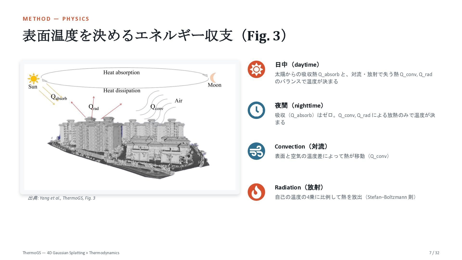
7. METHOD — PHYSICS 表面温度を決めるエネルギー収支（Fig. 3） 日中（daytime） 太陽からの吸収熱 Q_absorb と、対流・放射で失う熱 Q_conv, Q_rad のバランスで温度が決まる 夜間（nighttime） 吸収（Q_absorb）はゼロ。Q_conv, Q_rad による放熱のみで温度が決 まる Convection（対流） 表面と空気の温度差によって熱が移動（Q_conv） Radiation（放射） 出典: Yang et al., ThermoGS, Fig. 3 ThermoGS — 4D Gaussian Splatting × Thermodynamics 自己の温度の4乗に比例して熱を放出（Stefan–Boltzmann 則） 7 / 32
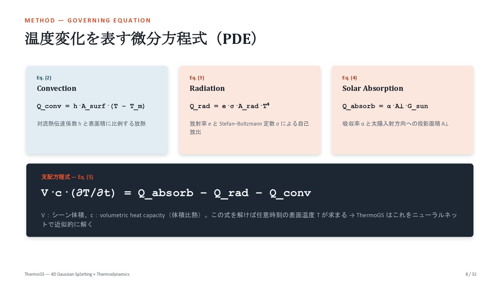
8. METHOD — GOVERNING EQUATION 温度変化を表す微分方程式（PDE） Eq. (2) Eq. (3) Eq. (4) Convection Radiation Solar Absorption Q_conv = h·A_surf·(T − T_m) Q_rad = e·σ·A_rad·T⁴ Q_absorb = α·A⊥·G_sun 対流熱伝達係数 h と表面積に比例する放熱 放射率 e と Stefan–Boltzmann 定数 σ による自己 放出 吸収率 α と太陽入射方向への投影面積 A⊥ 支配方程式 — Eq. (5) V·c·(∂T/∂t) = Q_absorb − Q_rad − Q_conv V：シーン体積、c：volumetric heat capacity（体積比熱）。この式を解けば任意時刻の表面温度 T が求まる → ThermoGS はこれをニューラルネッ トで近似的に解く ThermoGS — 4D Gaussian Splatting × Thermodynamics 8 / 32
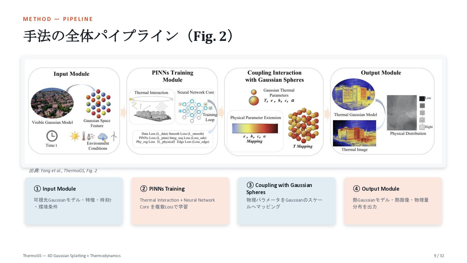
9. METHOD — PIPELINE 手法の全体パイプライン（Fig. 2） 出典: Yang et al., ThermoGS, Fig. 2 ① Input Module ② PINNs Training ③ Coupling with Gaussian Spheres ④ Output Module 可視光Gaussianモデル・特徴・時刻t ・環境条件 Thermal Interaction + Neural Network Core を複数Lossで学習 物理パラメータをGaussianのスケー ルへマッピング 熱Gaussianモデル・熱画像・物理量 分布を出力 ThermoGS — 4D Gaussian Splatting × Thermodynamics 9 / 32
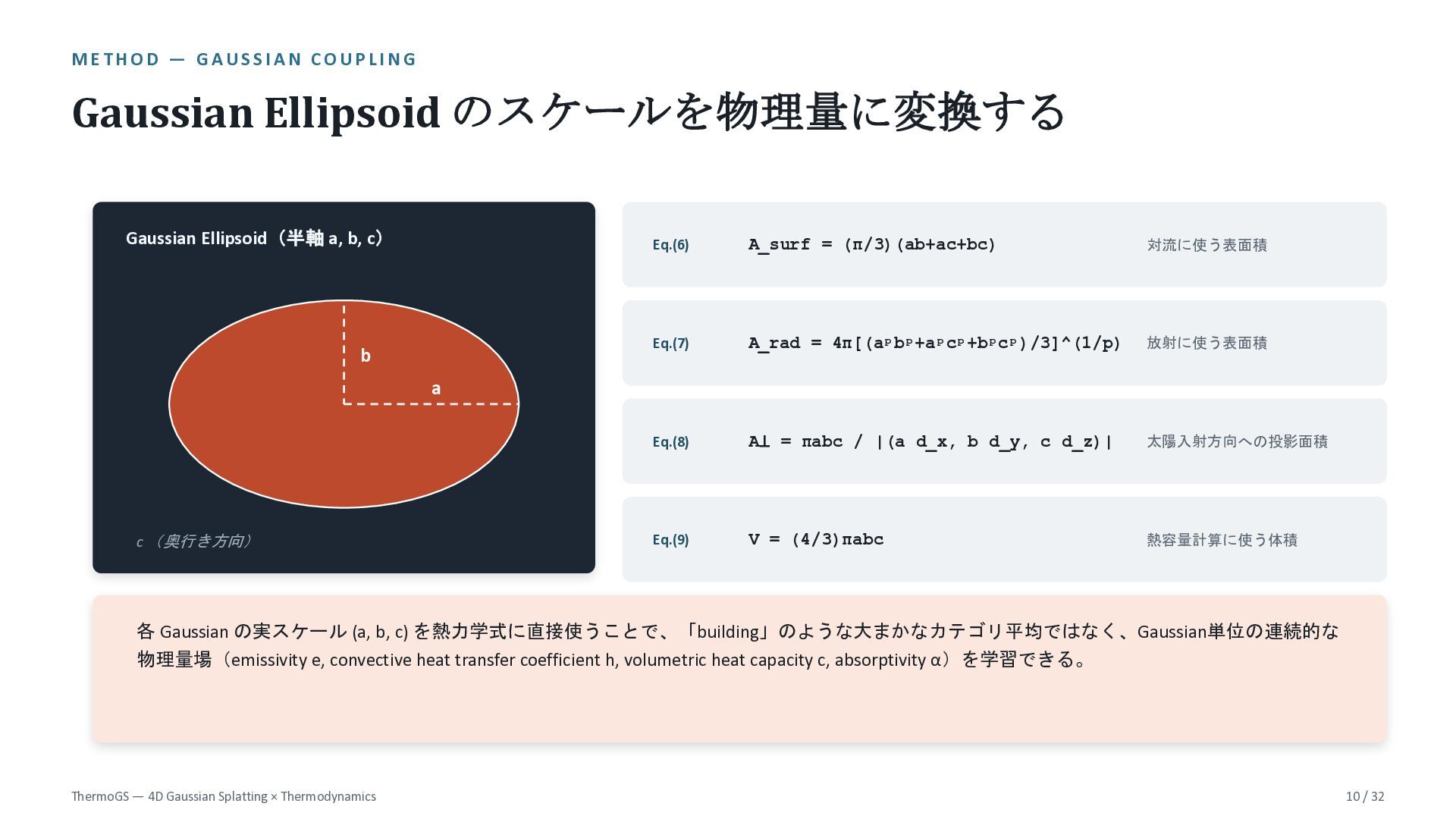
10. METHOD — GAUSSIAN COUPLING Gaussian Ellipsoid のスケールを物理量に変換する Gaussian Ellipsoid（半軸 a, b, c） b Eq.(6) A_surf = (π/3)(ab+ac+bc) 対流に使う表面積 Eq.(7) A_rad = 4π[(aᵖbᵖ+aᵖcᵖ+bᵖcᵖ)/3]^(1/p) 放射に使う表面積 Eq.(8) A⊥ = πabc / |(a d_x, b d_y, c d_z)| 太陽入射方向への投影面積 Eq.(9) V = (4/3)πabc 熱容量計算に使う体積 a c （奥行き方向） 各 Gaussian の実スケール (a, b, c) を熱力学式に直接使うことで、「building」のような大まかなカテゴリ平均ではなく、Gaussian単位の連続的な 物理量場（emissivity e, convective heat transfer coefficient h, volumetric heat capacity c, absorptivity α）を学習できる。 ThermoGS — 4D Gaussian Splatting × Thermodynamics 10 / 32
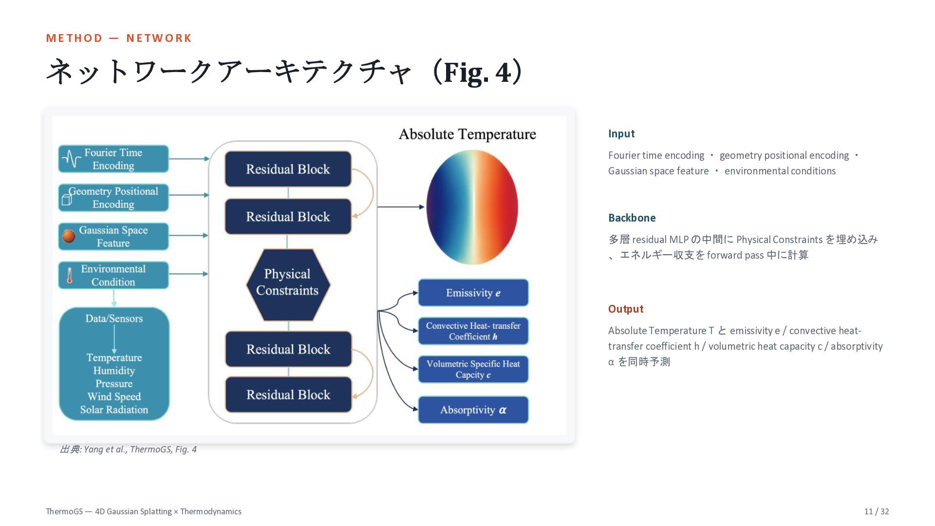
11. METHOD — NETWORK ネットワークアーキテクチャ（Fig. 4） Input Fourier time encoding ・ geometry positional encoding ・ Gaussian space feature ・ environmental conditions Backbone 多層 residual MLP の中間に Physical Constraints を埋め込み 、エネルギー収支を forward pass 中に計算 Output Absolute Temperature T と emissivity e / convective heattransfer coefficient h / volumetric heat capacity c / absorptivity α を同時予測 出典: Yang et al., ThermoGS, Fig. 4 ThermoGS — 4D Gaussian Splatting × Thermodynamics 11 / 32
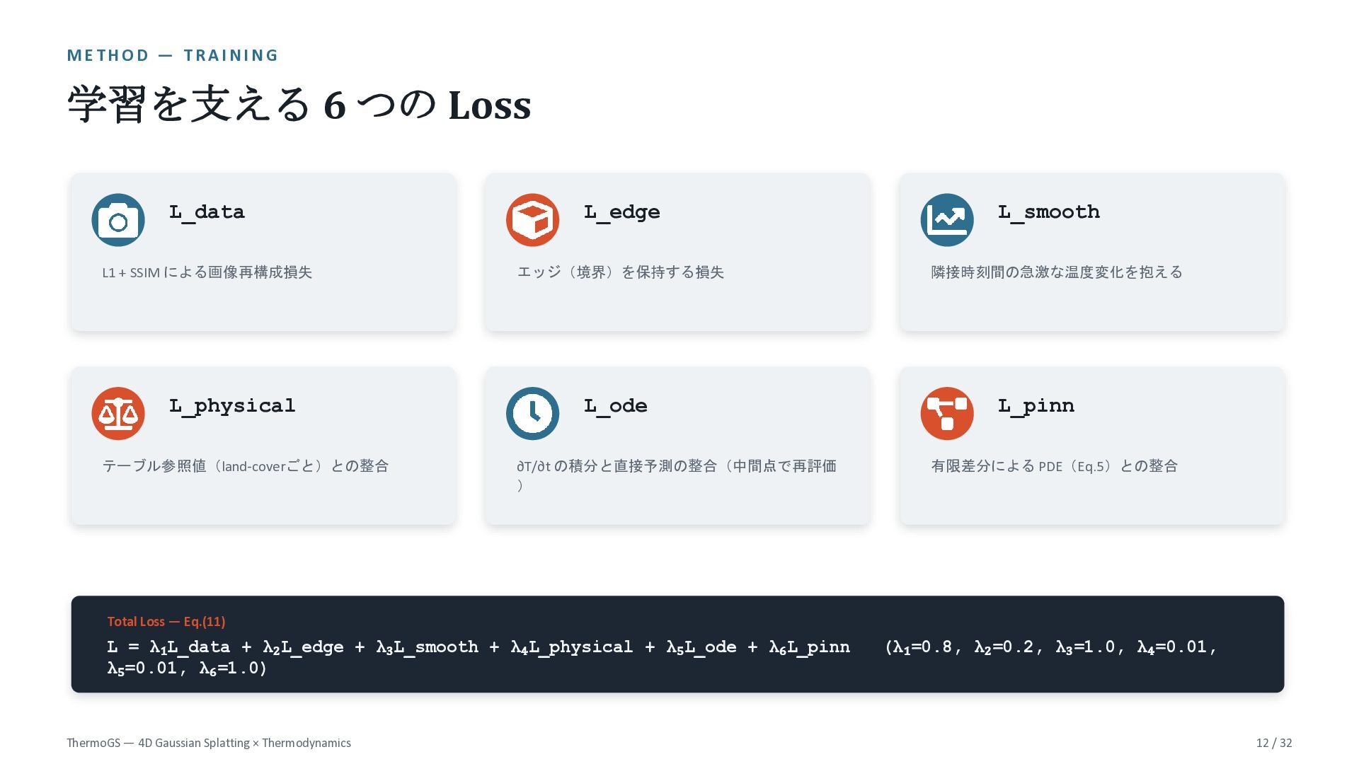
12. METHOD — TRAINING 学習を支える 6 つの Loss L_data L_edge L_smooth L1 + SSIM による画像再構成損失 エッジ（境界）を保持する損失 隣接時刻間の急激な温度変化を抱える L_physical テーブル参照値（land-coverごと）との整合 L_ode ∂T/∂t の積分と直接予測の整合（中間点で再評価 ） L_pinn 有限差分による PDE（Eq.5）との整合 Total Loss — Eq.(11) L = λ₁L_data + λ₂L_edge + λ₃L_smooth + λ₄L_physical + λ₅L_ode + λ₆L_pinn λ₅=0.01, λ₆=1.0) ThermoGS — 4D Gaussian Splatting × Thermodynamics (λ₁=0.8, λ₂=0.2, λ₃=1.0, λ₄=0.01, 12 / 32
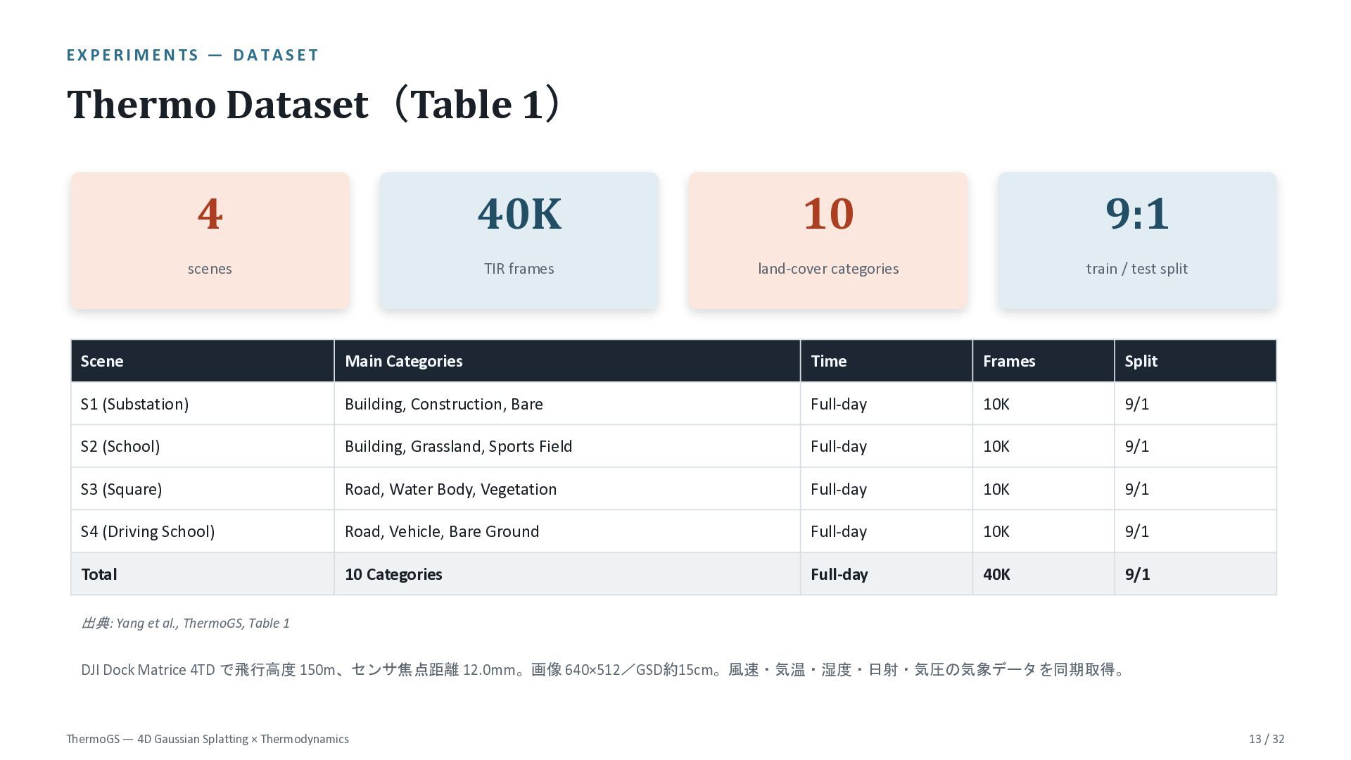
13. EXPERIMENTS — DATASET Thermo Dataset（Table 1） 4 40K 10 9:1 scenes TIR frames land-cover categories train / test split Scene Main Categories Time Frames Split S1 (Substation) Building, Construction, Bare Full-day 10K 9/1 S2 (School) Building, Grassland, Sports Field Full-day 10K 9/1 S3 (Square) Road, Water Body, Vegetation Full-day 10K 9/1 S4 (Driving School) Road, Vehicle, Bare Ground Full-day 10K 9/1 Total 10 Categories Full-day 40K 9/1 出典: Yang et al., ThermoGS, Table 1 DJI Dock Matrice 4TD で飛行高度 150m、センサ焦点距離 12.0mm。画像 640×512／GSD約15cm。風速・気温・湿度・日射・気圧の気象データを同期取得。 ThermoGS — 4D Gaussian Splatting × Thermodynamics 13 / 32
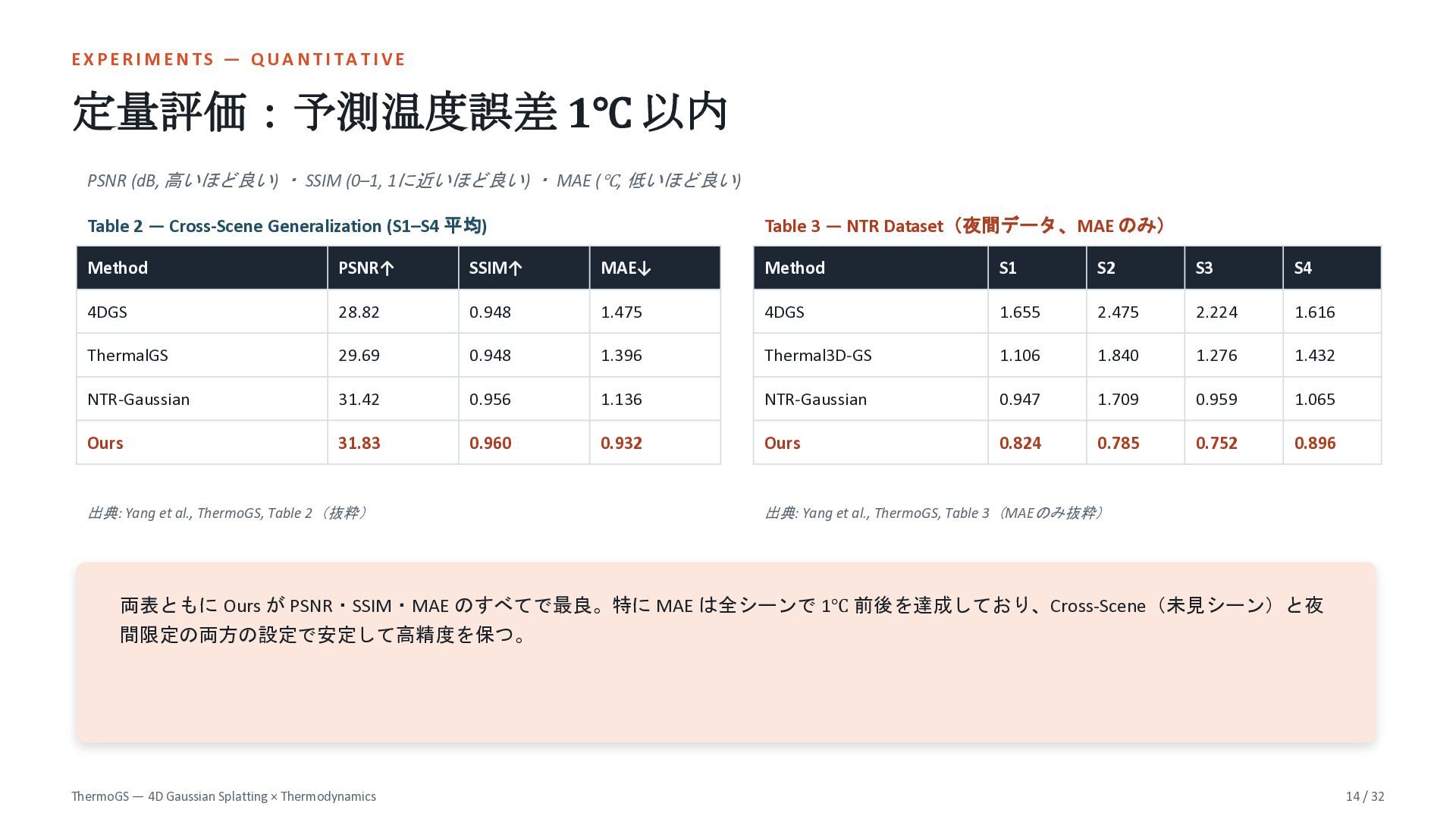
14. EXPERIMENTS — QUANTITATIVE 定量評価：予測温度誤差 1℃ 以内 PSNR (dB, 高いほど良い) ・ SSIM (0–1, 1に近いほど良い) ・ MAE (℃, 低いほど良い) Table 2 — Cross-Scene Generalization (S1–S4 平均) Table 3 — NTR Dataset（夜間データ、MAE のみ） Method PSNR↑ SSIM↑ MAE↓ Method S1 S2 S3 S4 4DGS 28.82 0.948 1.475 4DGS 1.655 2.475 2.224 1.616 ThermalGS 29.69 0.948 1.396 Thermal3D-GS 1.106 1.840 1.276 1.432 NTR-Gaussian 31.42 0.956 1.136 NTR-Gaussian 0.947 1.709 0.959 1.065 Ours 31.83 0.960 0.932 Ours 0.824 0.785 0.752 0.896 出典: Yang et al., ThermoGS, Table 2（抜粋） 出典: Yang et al., ThermoGS, Table 3（MAEのみ抜粋） 両表ともに Ours が PSNR・SSIM・MAE のすべてで最良。特に MAE は全シーンで 1℃ 前後を達成しており、Cross-Scene（未見シーン）と夜 間限定の両方の設定で安定して高精度を保つ。 ThermoGS — 4D Gaussian Splatting × Thermodynamics 14 / 32
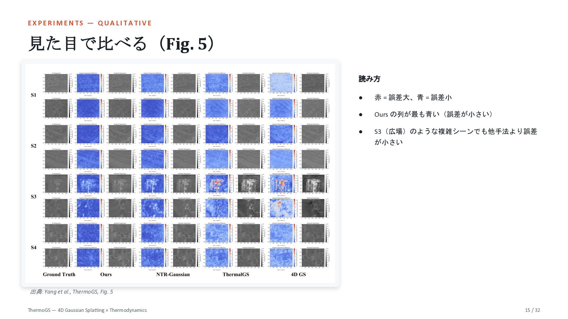
15. EXPERIMENTS — QUALITATIVE 見た目で比べる（Fig. 5） 読み方 • 赤 = 誤差大、青 = 誤差小 • Ours の列が最も青い（誤差が小さい） • S3（広場）のような複雑シーンでも他手法より誤差 が小さい 出典: Yang et al., ThermoGS, Fig. 5 ThermoGS — 4D Gaussian Splatting × Thermodynamics 15 / 32
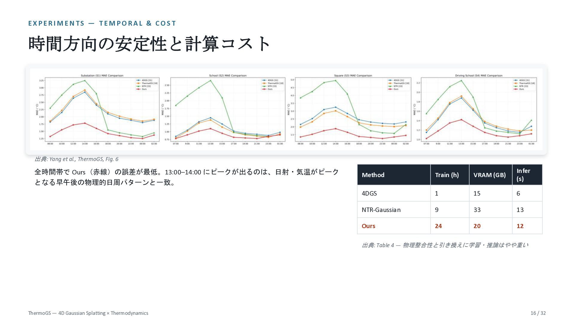
16. EXPERIMENTS — TEMPORAL & COST 時間方向の安定性と計算コスト 出典: Yang et al., ThermoGS, Fig. 6 全時間帯で Ours（赤線）の誤差が最低。13:00–14:00 にピークが出るのは、日射・気温がピーク となる早午後の物理的日周パターンと一致。 Method Train (h) VRAM (GB) Infer (s) 4DGS 1 15 6 NTR-Gaussian 9 33 13 Ours 24 20 12 出典: Table 4 — 物理整合性と引き換えに学習・推論はやや重い ThermoGS — 4D Gaussian Splatting × Thermodynamics 16 / 32
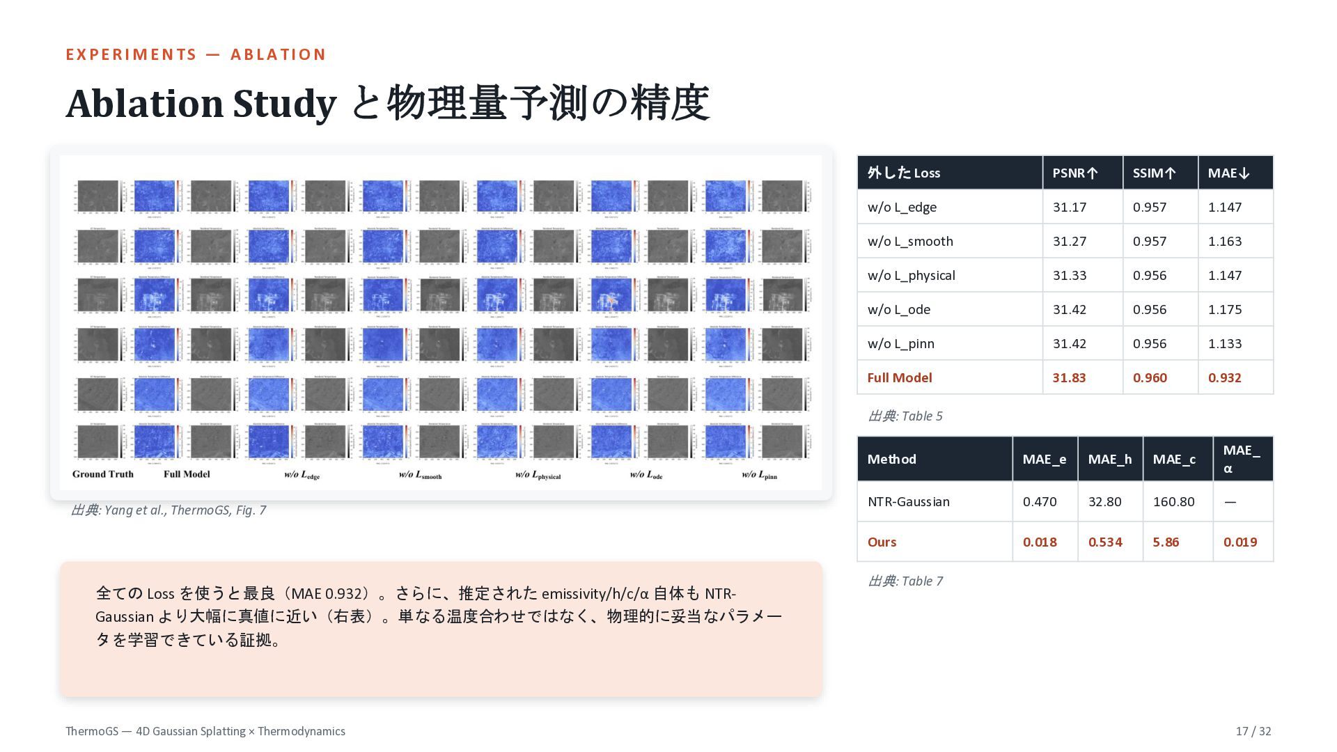
17. EXPERIMENTS — ABLATION Ablation Study と物理量予測の精度 外した Loss PSNR↑ SSIM↑ MAE↓ w/o L_edge 31.17 0.957 1.147 w/o L_smooth 31.27 0.957 1.163 w/o L_physical 31.33 0.956 1.147 w/o L_ode 31.42 0.956 1.175 w/o L_pinn 31.42 0.956 1.133 Full Model 31.83 0.960 0.932 出典: Table 5 出典: Yang et al., ThermoGS, Fig. 7 全ての Loss を使うと最良（MAE 0.932）。さらに、推定された emissivity/h/c/α 自体も NTRGaussian より大幅に真値に近い（右表）。単なる温度合わせではなく、物理的に妥当なパラメー タを学習できている証拠。 ThermoGS — 4D Gaussian Splatting × Thermodynamics Method MAE_e MAE_h MAE_c MAE_ α NTR-Gaussian 0.470 32.80 160.80 — Ours 0.018 0.534 5.86 0.019 出典: Table 7 17 / 32
18. TAKEAWAYS まとめ 4D Gaussian Splatting + 熱力学（Physics-Informed Neural Networks）を統合 「再現（Reproduce）」ではなく「シミュレーション（Simulate）」を実現 放射輝度を直接予測せず、物理量を decouple emissivity ・ convective heat transfer coefficient ・ volumetric heat capacity ・ absorptivity を温度から分離 → 解釈性・汎化性が向上 Gaussian Ellipsoid の実スケールを物理式に統合 カテゴリ平均ではなく、連続的な物理量場（continuous physical manifold）を学習 新データセット Thermo Dataset（4シーン・約40K枚・終日） 対応 GitHub： github.com/NPU-CVPG/ThermoGS（現時点では README のみでデータは未公開） CV 研究への示唆 Physics-Informed Learning は「見た目が近い」だけでなく「物理的に正しい」生成モデルを作る有力な設計パターン ThermoGS — 4D Gaussian Splatting × Thermodynamics 18 / 32
19. THANK YOU Q&A ご清聴ありがとうございました。 Reference Kun Yang, Yuxiang Liu, Zeyu Cui, Shen Yan, Maojun Zhang, Yu Liu, Xue Wang, Qing Wang. “ThermoGS: Decoupling Physical Surface Attributes for Spatio-Temporal Thermal Field Emulation via 4D Gaussian Splatting.” Springer (DOI: 10.1007/978-3-03237429-5_18). Code: github.com/NPU-CVPG/ThermoGS · 本デッキの図・表は全て原論文から引用・作成・本スライド作成にはClaude使用 ThermoGS — 4D Gaussian Splatting × Thermodynamics 19 / 32