Guaranteed, Adaptive, Automatic Algorithms for Univariate Integration: Methods, Costs and Implementations

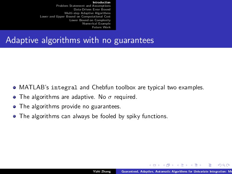
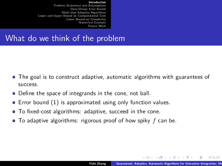
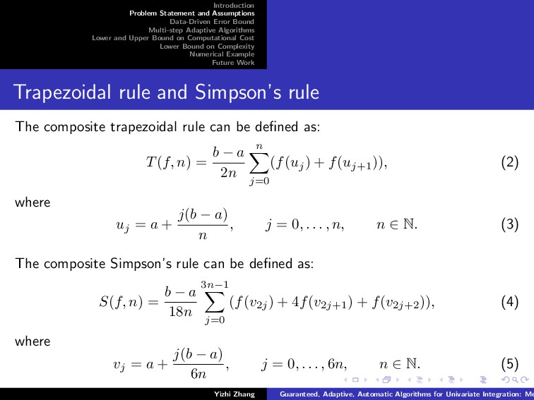
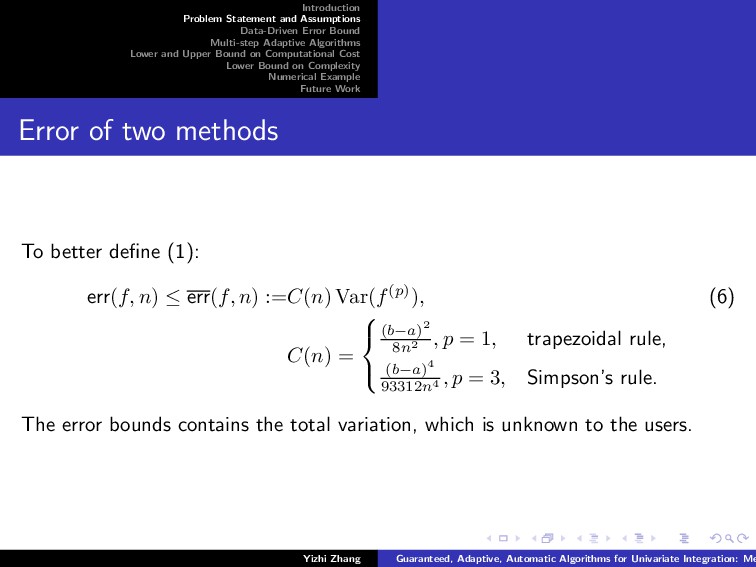
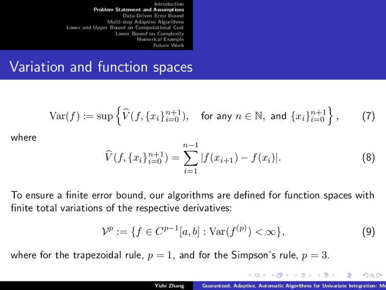
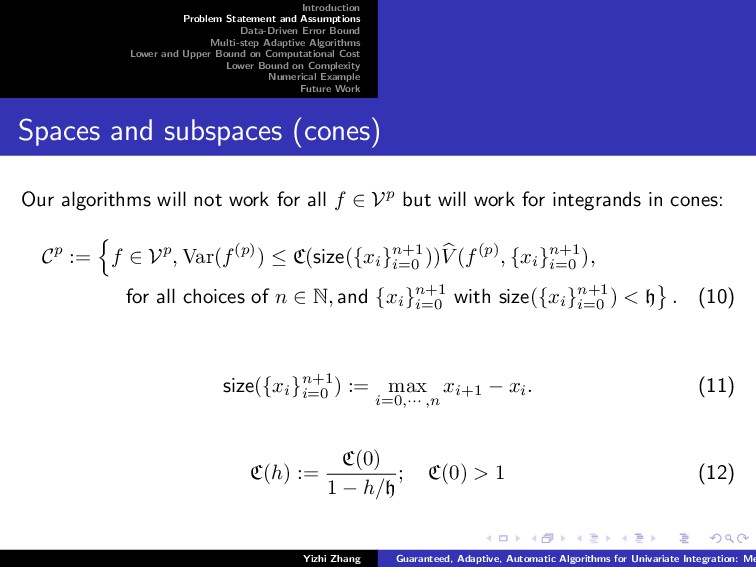
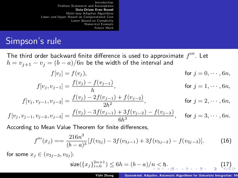
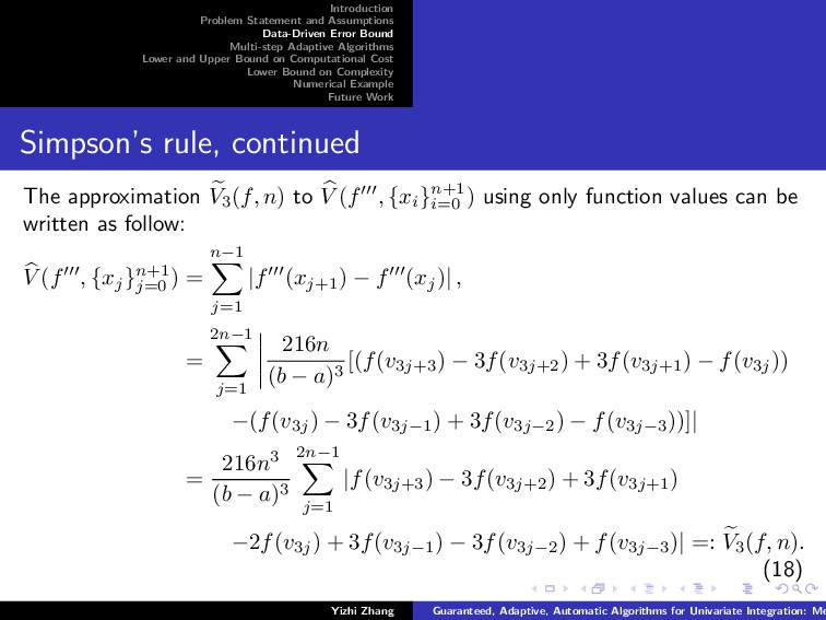
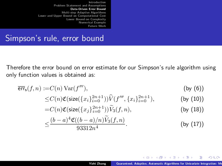
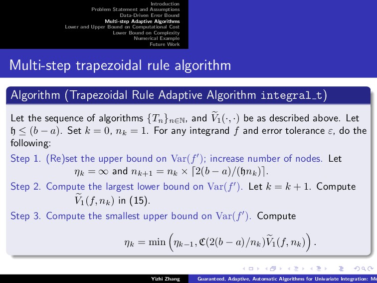
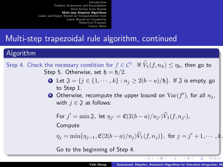
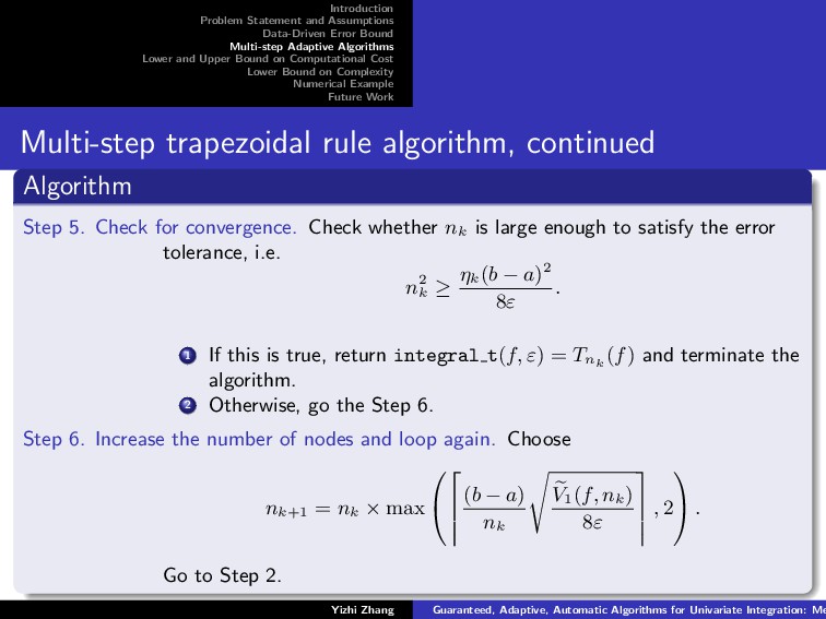
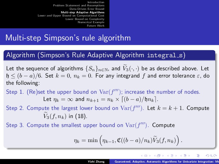
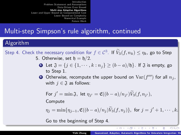
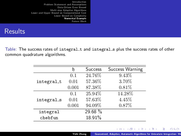
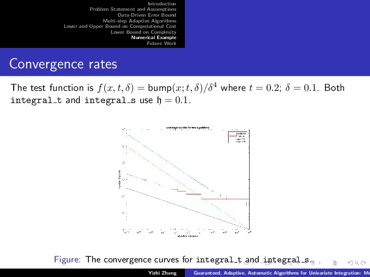
Slides presented Yizhi Zhang's PhD oral defense exam for his work on his PhD thesis. This thesis investigates how to solve univariate integration problems using numerical methods, including the trapezoidal rule and the Simpson's rule. Most existing guaranteed algorithms are not adaptive and require too much a priori information. Most existing adaptive algorithms do not have valid justification for their results. The goal is to create adaptive algorithms utilizing the two above-mentioned methods with guarantees. The classes of integrands studied in this thesis are cones. The algorithms are analytically proved to be a success if the integrand lies in the cone. The algorithms are adaptive and automatically adjust the computational costs based on the integrand values. The lower and upper bounds on the computational costs for both algorithms are derived. The lower bounds on the complexity of the problems are derived as well. By comparing the upper bounds on the computational cost and the lower bounds on the complexity, our algorithms are shown to be asymptotically optimal. Numerical experiments are implemented.

Transcript

1. Introduction Problem Statement and Assumptions Data-Driven Error Bound Multi-step Adaptive Algorithms Lower and Upper Bound on Computational Cost Lower Bound on Complexity Numerical Example Future Work Guaranteed, Adaptive, Automatic Algorithms for Univariate Integration: Methods, Cost and Implementation Yizhi Zhang Department of Applied Mathematics, Illinois Institute of Technology October 29, 2018 Yizhi Zhang Guaranteed, Adaptive, Automatic Algorithms for Univariate Integration: Me
2. Introduction Problem Statement and Assumptions Data-Driven Error Bound Multi-step Adaptive Algorithms Lower and Upper Bound on Computational Cost Lower Bound on Complexity Numerical Example Future Work Contents Introduction . . . . . . . Yizhi Zhang Guaranteed, Adaptive, Automatic Algorithms for Univariate Integration: Me
3. Introduction Problem Statement and Assumptions Data-Driven Error Bound Multi-step Adaptive Algorithms Lower and Upper Bound on Computational Cost Lower Bound on Complexity Numerical Example Future Work Motivation b a f(x)dx Simple functions such as b a x2dx = x3/3|b a . Use pen and paper. Functions with no analytical solutions such as the standard normal p.d.f b a e−x2/2/ √ 2πdx. Use numerical methods. Yizhi Zhang Guaranteed, Adaptive, Automatic Algorithms for Univariate Integration: Me
4. Introduction Problem Statement and Assumptions Data-Driven Error Bound Multi-step Adaptive Algorithms Lower and Upper Bound on Computational Cost Lower Bound on Complexity Numerical Example Future Work Fixed-cost algorithms The traditional trapezoidal rule and Simpson’s rule are typical two examples. err(f, n) ≤ err(f, n) :=C(n) Var(f(p)), (1) The algorithms provide guarantees when Var(f(p)) < σ. The algorithms are automatic. Cost n = C−1(ε/σ). The algorithms are not adaptive. The upper bound on variation, σ is not dependent on the integrand. A constant c · f may not work. Yizhi Zhang Guaranteed, Adaptive, Automatic Algorithms for Univariate Integration: Me
5. Introduction Problem Statement and Assumptions Data-Driven Error Bound Multi-step Adaptive Algorithms Lower and Upper Bound on Computational Cost Lower Bound on Complexity Numerical Example Future Work Adaptive algorithms with no guarantees MATLAB’s integral and Chebfun toolbox are typical two examples. The algorithms are adaptive. No σ required. The algorithms provide no guarantees. The algorithms can always be fooled by spiky functions. Yizhi Zhang Guaranteed, Adaptive, Automatic Algorithms for Univariate Integration: Me
6. Introduction Problem Statement and Assumptions Data-Driven Error Bound Multi-step Adaptive Algorithms Lower and Upper Bound on Computational Cost Lower Bound on Complexity Numerical Example Future Work What do we think of the problem The goal is to construct adaptive, automatic algorithms with guarantees of success. Define the space of integrands in the cone, not ball. Error bound (1) is approximated using only function values. To fixed-cost algorithms: adaptive, succeed in the cone. To adaptive algorithms: rigorous proof of how spiky f can be. Yizhi Zhang Guaranteed, Adaptive, Automatic Algorithms for Univariate Integration: Me
7. Introduction Problem Statement and Assumptions Data-Driven Error Bound Multi-step Adaptive Algorithms Lower and Upper Bound on Computational Cost Lower Bound on Complexity Numerical Example Future Work Contents Introduction Problem Statement Data-Driven Error Bounds Multi-step Adaptive Algorithms Lower and Upper Bound on Computational Cost Lower Bound on Complexity Numerical Example Future Work Yizhi Zhang Guaranteed, Adaptive, Automatic Algorithms for Univariate Integration: Me
8. Introduction Problem Statement and Assumptions Data-Driven Error Bound Multi-step Adaptive Algorithms Lower and Upper Bound on Computational Cost Lower Bound on Complexity Numerical Example Future Work work flow Yizhi Zhang Guaranteed, Adaptive, Automatic Algorithms for Univariate Integration: Me
9. Introduction Problem Statement and Assumptions Data-Driven Error Bound Multi-step Adaptive Algorithms Lower and Upper Bound on Computational Cost Lower Bound on Complexity Numerical Example Future Work Trapezoidal rule and Simpson’s rule The composite trapezoidal rule can be defined as: T(f, n) = b − a 2n n j=0 (f(uj ) + f(uj+1 )), (2) where uj = a + j(b − a) n , j = 0, . . . , n, n ∈ N. (3) The composite Simpson’s rule can be defined as: S(f, n) = b − a 18n 3n−1 j=0 (f(v2j ) + 4f(v2j+1 ) + f(v2j+2 )), (4) where vj = a + j(b − a) 6n , j = 0, . . . , 6n, n ∈ N. (5) Yizhi Zhang Guaranteed, Adaptive, Automatic Algorithms for Univariate Integration: Me
10. Introduction Problem Statement and Assumptions Data-Driven Error Bound Multi-step Adaptive Algorithms Lower and Upper Bound on Computational Cost Lower Bound on Complexity Numerical Example Future Work Error of two methods To better define (1): err(f, n) ≤ err(f, n) :=C(n) Var(f(p)), (6) C(n) =    (b−a)2 8n2 , p = 1, trapezoidal rule, (b−a)4 93312n4 , p = 3, Simpson’s rule. The error bounds contains the total variation, which is unknown to the users. Yizhi Zhang Guaranteed, Adaptive, Automatic Algorithms for Univariate Integration: Me
11. Introduction Problem Statement and Assumptions Data-Driven Error Bound Multi-step Adaptive Algorithms Lower and Upper Bound on Computational Cost Lower Bound on Complexity Numerical Example Future Work Variation and function spaces Var(f) := sup V (f, {xi }n+1 i=0 ), for any n ∈ N, and {xi }n+1 i=0 , (7) where V (f, {xi }n+1 i=0 ) = n−1 i=1 |f(xi+1 ) − f(xi )|. (8) To ensure a finite error bound, our algorithms are defined for function spaces with finite total variations of the respective derivatives: Vp := {f ∈ Cp−1[a, b] : Var(f(p)) < ∞}, (9) where for the trapezoidal rule, p = 1, and for the Simpson’s rule, p = 3. Yizhi Zhang Guaranteed, Adaptive, Automatic Algorithms for Univariate Integration: Me
12. Introduction Problem Statement and Assumptions Data-Driven Error Bound Multi-step Adaptive Algorithms Lower and Upper Bound on Computational Cost Lower Bound on Complexity Numerical Example Future Work Spaces and subspaces (cones) Our algorithms will not work for all f ∈ Vp but will work for integrands in cones: Cp := f ∈ Vp, Var(f(p)) ≤ C(size({xi }n+1 i=0 ))V (f(p), {xi }n+1 i=0 ), for all choices of n ∈ N, and {xi }n+1 i=0 with size({xi }n+1 i=0 ) < h . (10) size({xi }n+1 i=0 ) := max i=0,··· ,n xi+1 − xi . (11) C(h) := C(0) 1 − h/h ; C(0) > 1 (12) Yizhi Zhang Guaranteed, Adaptive, Automatic Algorithms for Univariate Integration: Me
13. Introduction Problem Statement and Assumptions Data-Driven Error Bound Multi-step Adaptive Algorithms Lower and Upper Bound on Computational Cost Lower Bound on Complexity Numerical Example Future Work How to find error bounds The definition of the cone suggests a way of bounding Var(f(p)) in terms of V (f(p), {xi }n+1 i=0 ). Our algorithms are based on function values and V (f(p), {xi }n+1 i=0 ) is defined in terms of derivative values. Find a way to express derivative values in terms of function values. Yizhi Zhang Guaranteed, Adaptive, Automatic Algorithms for Univariate Integration: Me
14. Introduction Problem Statement and Assumptions Data-Driven Error Bound Multi-step Adaptive Algorithms Lower and Upper Bound on Computational Cost Lower Bound on Complexity Numerical Example Future Work Trapezoidal rule The backward finite difference is used to approximate f . Let the width of the interval h = uj+1 − uj = (b − a)/n and f[uj ] = f(uj ), for j = 0, · · · , n, f[uj , uj−1 ] = f(uj ) − f(uj−1 ) h , for j = 1, · · · , n. According to Mean Value Theorem for finite differences, f (xj ) = f(uj ) − f(uj−1 ) h = n b − a [f(uj ) − f(uj−1 )], (13) for some xj ∈ (uj−1 , uj ). size({xj }n+1 j=0 ) ≤ 2h = 2(b − a)/n < h. (14) Yizhi Zhang Guaranteed, Adaptive, Automatic Algorithms for Univariate Integration: Me
15. Introduction Problem Statement and Assumptions Data-Driven Error Bound Multi-step Adaptive Algorithms Lower and Upper Bound on Computational Cost Lower Bound on Complexity Numerical Example Future Work Trapezoidal rule, continued The approximation V1 (f, n) to V (f , {xj }n+1 i=0 ) using only function values is defined as: V (f , {xj }n+1 j=0 ) = n−1 j=1 |f (xj+1 ) − f (xj )| , = n−1 j=1 n b − a [f(uj+1 ) − f(uj ) − f(uj ) + f(uj−1 )] = n b − a n−1 j=1 |f(uj+1 ) − 2f(uj ) + f(uj−1 )| =: V1 (f, n). (15) Yizhi Zhang Guaranteed, Adaptive, Automatic Algorithms for Univariate Integration: Me
16. Introduction Problem Statement and Assumptions Data-Driven Error Bound Multi-step Adaptive Algorithms Lower and Upper Bound on Computational Cost Lower Bound on Complexity Numerical Example Future Work Trapezoidal rule, error bound errt(f, n) :=C(n) Var(f ), (by (6)) ≤C(n)C(size({xi }n+1 i=0 ))V (f , {xi }n+1 i=0 ), (by (10)) =C(n)C(size({xj }n+1 i=0 ))V1 (f, n), (by (15)) ≤ (b − a)2C(2(b − a)/n)V1 (f, n) 8n2 . (by (14)) Yizhi Zhang Guaranteed, Adaptive, Automatic Algorithms for Univariate Integration: Me
17. Introduction Problem Statement and Assumptions Data-Driven Error Bound Multi-step Adaptive Algorithms Lower and Upper Bound on Computational Cost Lower Bound on Complexity Numerical Example Future Work Simpson’s rule The third order backward finite difference is used to approximate f . Let h = vj+1 − vj = (b − a)/6n be the width of the interval and f[vj ] = f(vj ), for j = 0, · · · , 6n, f[vj , vj−1 ] = f(vj ) − f(vj−1 ) h , for j = 1, · · · , 6n, f[vj , vj−1 , vj−2 ] = f(vj ) − 2f(vj−1 ) + f(vj−2 ) 2h2 , for j = 2, · · · , 6n, f[vj , vj−1 , vj−2 , vj−3 ] = f(vj ) − 3f(vj−1 ) + 3f(vj−2 ) − f(vj−3 ) 6h3 , for j = 3, · · · , 6n. According to Mean Value Theorem for finite differences, f (xj ) == 216n3 (b − a)3 [f(v3j ) − 3f(v3j−1 ) + 3f(v3j−2 ) − f(v3j−3 )]. (16) for some xj ∈ (v3j−3 , v3j ). size({xj }2n+1 i=0 ) ≤ 6h = (b − a)/n < h. (17) Yizhi Zhang Guaranteed, Adaptive, Automatic Algorithms for Univariate Integration: Me
18. Introduction Problem Statement and Assumptions Data-Driven Error Bound Multi-step Adaptive Algorithms Lower and Upper Bound on Computational Cost Lower Bound on Complexity Numerical Example Future Work Simpson’s rule, continued The approximation V3 (f, n) to V (f , {xi }n+1 i=0 ) using only function values can be written as follow: V (f , {xj }n+1 j=0 ) = n−1 j=1 |f (xj+1 ) − f (xj )| , = 2n−1 j=1 216n (b − a)3 [(f(v3j+3 ) − 3f(v3j+2 ) + 3f(v3j+1 ) − f(v3j )) −(f(v3j ) − 3f(v3j−1 ) + 3f(v3j−2 ) − f(v3j−3 ))]| = 216n3 (b − a)3 2n−1 j=1 |f(v3j+3 ) − 3f(v3j+2 ) + 3f(v3j+1 ) −2f(v3j ) + 3f(v3j−1 ) − 3f(v3j−2 ) + f(v3j−3 )| =: V3 (f, n). (18) Yizhi Zhang Guaranteed, Adaptive, Automatic Algorithms for Univariate Integration: Me
19. Introduction Problem Statement and Assumptions Data-Driven Error Bound Multi-step Adaptive Algorithms Lower and Upper Bound on Computational Cost Lower Bound on Complexity Numerical Example Future Work Simpson’s rule, error bound Therefore the error bound on error estimate for our Simpson’s rule algorithm using only function values is obtained as: errs(f, n) :=C(n) Var(f ), (by (6)) ≤C(n)C(size({xi }2n+1 i=0 ))V (f , {xi }2n+1 i=0 ), (by (10)) =C(n)C(size({xj }2n+1 i=0 ))V3 (f, n), (by (18)) ≤ (b − a)4C((b − a)/n)V3 (f, n) 93312n4 . (by (17)) Yizhi Zhang Guaranteed, Adaptive, Automatic Algorithms for Univariate Integration: Me
20. Introduction Problem Statement and Assumptions Data-Driven Error Bound Multi-step Adaptive Algorithms Lower and Upper Bound on Computational Cost Lower Bound on Complexity Numerical Example Future Work Multi-step trapezoidal rule algorithm Algorithm (Trapezoidal Rule Adaptive Algorithm integral t) Let the sequence of algorithms {Tn }n∈N , and V1 (·, ·) be as described above. Let h ≤ (b − a). Set k = 0, nk = 1. For any integrand f and error tolerance ε, do the following: Step 1. (Re)set the upper bound on Var(f ); increase number of nodes. Let ηk = ∞ and nk+1 = nk × 2(b − a)/(hnk ) . Step 2. Compute the largest lower bound on Var(f ). Let k = k + 1. Compute V1 (f, nk ) in (15). Step 3. Compute the smallest upper bound on Var(f ). Compute ηk = min ηk−1 , C(2(b − a)/nk )V1 (f, nk ) . Yizhi Zhang Guaranteed, Adaptive, Automatic Algorithms for Univariate Integration: Me
21. Introduction Problem Statement and Assumptions Data-Driven Error Bound Multi-step Adaptive Algorithms Lower and Upper Bound on Computational Cost Lower Bound on Complexity Numerical Example Future Work Multi-step trapezoidal rule algorithm, continued Algorithm Step 4. Check the necessary condition for f ∈ C1. If V1 (f, nk ) ≤ ηk , then go to Step 5. Otherwise, set h = h/2. 1 Let J = {j ∈ {1, · · · , k} : nj ≥ 2(b − a)/h}. If J is empty, go to Step 1. 2 Otherwise, recompute the upper bound on Var(f ), for all nj , with j ∈ J as follows: For j = min J, let ηj = C(2(b − a)/nj )V1 (f, nj ), Compute ηj = min{ηj−1 , C(2(b − a)/nj )V1 (f, nj )}, for j = j + 1, · · · , k. Go to the beginning of Step 4. Yizhi Zhang Guaranteed, Adaptive, Automatic Algorithms for Univariate Integration: Me
22. Introduction Problem Statement and Assumptions Data-Driven Error Bound Multi-step Adaptive Algorithms Lower and Upper Bound on Computational Cost Lower Bound on Complexity Numerical Example Future Work Multi-step trapezoidal rule algorithm, continued Algorithm Step 5. Check for convergence. Check whether nk is large enough to satisfy the error tolerance, i.e. n2 k ≥ ηk (b − a)2 8ε . 1 If this is true, return integral t(f, ε) = Tnk (f) and terminate the algorithm. 2 Otherwise, go the Step 6. Step 6. Increase the number of nodes and loop again. Choose nk+1 = nk × max       (b − a) nk V1 (f, nk ) 8ε     , 2   . Go to Step 2. Yizhi Zhang Guaranteed, Adaptive, Automatic Algorithms for Univariate Integration: Me
23. Introduction Problem Statement and Assumptions Data-Driven Error Bound Multi-step Adaptive Algorithms Lower and Upper Bound on Computational Cost Lower Bound on Complexity Numerical Example Future Work Multi-step Simpson’s rule algorithm Algorithm (Simpson’s Rule Adaptive Algorithm integral s) Let the sequence of algorithms {Sn }n∈N , and V3 (·, ·) be as described above. Let h ≤ (b − a)/6. Set k = 0, nk = 0. For any integrand f and error tolerance ε, do the following: Step 1. (Re)set the upper bound on Var(f ); increase the number of nodes. Let ηk = ∞ and nk+1 = nk × (b − a)/hnk . Step 2. Compute the largest lower bound on Var(f ). Let k = k + 1. Compute V3 (f, nk ) in (18). Step 3. Compute the smallest upper bound on Var(f ). Compute ηk = min ηk−1 , C((b − a)/nk )V3 (f, nk ) . Yizhi Zhang Guaranteed, Adaptive, Automatic Algorithms for Univariate Integration: Me
24. Introduction Problem Statement and Assumptions Data-Driven Error Bound Multi-step Adaptive Algorithms Lower and Upper Bound on Computational Cost Lower Bound on Complexity Numerical Example Future Work Multi-step Simpson’s rule algorithm, continued Algorithm Step 4. Check the necessary condition for f ∈ C3. If V3 (f, nk ) ≤ ηk , go to Step 5. Otherwise, set h = h/2. 1 Let J = {j ∈ {1, · · · , k : nj } ≥ (b − a)/h}. If J is empty, go to Step 1. 2 Otherwise, recompute the upper bound on Var(f ) for all nj , with j ∈ J as follows: For j = min J, let ηj = C((b − a)/nj )V3 (f, nj ), Compute ηj = min{ηj−1 , C((b − a)/nj )V3 (f, nj )}, for j = j + 1, · · · , k. Go to the beginning of Step 4. Yizhi Zhang Guaranteed, Adaptive, Automatic Algorithms for Univariate Integration: Me
25. Introduction Problem Statement and Assumptions Data-Driven Error Bound Multi-step Adaptive Algorithms Lower and Upper Bound on Computational Cost Lower Bound on Complexity Numerical Example Future Work Multi-step Simpson’s rule algorithm, continued Algorithm Step 5. Check for convergence. Check whether nk is large enough to satisfy the error tolerance, i.e. n4 k ≥ ηk (b − a)4 93312ε . 1 If true, return integral s(f, ε) = Snk (f) and terminate the algorithm. 2 Otherwise, go the Step 6. Step 6. Increase the number of nodes and loop again. Choose nk+1 = nk × max       (b − a) nk V3 (f, nk ) 93312ε 1/4    , 2   . Go to Step 2. Yizhi Zhang Guaranteed, Adaptive, Automatic Algorithms for Univariate Integration: Me
26. Introduction Problem Statement and Assumptions Data-Driven Error Bound Multi-step Adaptive Algorithms Lower and Upper Bound on Computational Cost Lower Bound on Complexity Numerical Example Future Work Computational cost of the trapezoidal rule Theorem Let N(f, ε) denote the final number nk in Step 5 when integral t terminates. Then this number is bounded below and above in terms of the true, yet unknown, Var(f ). max 2(b − a) h , 2(b − a) Var(f ) 8ε ≤ N(f, ε) ≤ 2 min n ∈ N : n ≥ 2(b − a) h , ζ(n) Var(f ) ≤ ε ≤ 2 min 0<α≤1 max 2(b − a) αh , (b − a) C(αh) Var(f ) 8ε , (19) where ζ(n) = (b − a)2C(2(b − a)/n)/(8εn2). The number of function values, namely, the computational cost required by the algorithm, is N(f, ε) + 1. Yizhi Zhang Guaranteed, Adaptive, Automatic Algorithms for Univariate Integration: Me
27. Introduction Problem Statement and Assumptions Data-Driven Error Bound Multi-step Adaptive Algorithms Lower and Upper Bound on Computational Cost Lower Bound on Complexity Numerical Example Future Work Computational cost of the Simpson’s rule Theorem Let N(f, ε) denote the final number of nk in Step 5 when integral s terminates. Then this number is bounded below and above in terms of the true, yet unknown, Var(f ). max (b − a) h , (b − a) Var(f ) 93312ε 1/4 ≤ N(f, ε) ≤ 2 min n ∈ N : n ≥ (b − a) h , ζ(n) Var(f ) ≤ ε ≤ 2 min 0<α≤1 max (b − a) αh , (b − a) C(αh) Var(f ) 93312ε 1/4 , (20) where ζ(n) = (b − a)4C((b − a)/n)/(93312n4). The number of function values, namely the computational cost, required by the algorithm is 6N(f, ε) + 1. Yizhi Zhang Guaranteed, Adaptive, Automatic Algorithms for Univariate Integration: Me
28. Introduction Problem Statement and Assumptions Data-Driven Error Bound Multi-step Adaptive Algorithms Lower and Upper Bound on Computational Cost Lower Bound on Complexity Numerical Example Future Work Computational cost of the Simpson’s rule, continued Proof. No matter what inputs f and ε are provided, N(f, ε) ≥ n1 = (b − a)/h . Then the number of intervals increases until err(f, n) ≤ ε. From the error bound defined in (6), C(N(f, ε)) Var(f ) ≤ ε. Thus N(f, ε) ≥ (b − a) Var(f ) 93312ε 1/4 . This implies the lower bound on N(f, ε). Yizhi Zhang Guaranteed, Adaptive, Automatic Algorithms for Univariate Integration: Me
29. Introduction Problem Statement and Assumptions Data-Driven Error Bound Multi-step Adaptive Algorithms Lower and Upper Bound on Computational Cost Lower Bound on Complexity Numerical Example Future Work Computational cost of the Simpson’s rule, continued Proof. Let K be the value of k for which integral s terminates. Since n1 satisfies the upper bound, one may assume that K ≥ 2. Let m be the multiplication integer found in Step 6. Note that ζ((m − 1)nK−1 ) Var(f ) > ε. For m = 2, this is true because ζ(nK−1 ) Var(f ) ≥ ζ(nK−1 )V3 (f, nK−1 ) > ε. For m > 2 it is true because of the definition of m. Since ζ is a decreasing function, it follows that (m − 1)nK−1 < n∗ := min n ∈ N : n ≥ 2(b − a) n , ζ(n) Var(f ) ≤ ε . Therefore nK = m∗nK−1 < m∗ n∗ m−1 = m m−1 n∗ ≤ 2n∗. Yizhi Zhang Guaranteed, Adaptive, Automatic Algorithms for Univariate Integration: Me
30. Introduction Problem Statement and Assumptions Data-Driven Error Bound Multi-step Adaptive Algorithms Lower and Upper Bound on Computational Cost Lower Bound on Complexity Numerical Example Future Work Computational cost of the Simpson’s rule, continued Proof. For fixed α ∈ (0, 1], we only need to consider that case where n∗ > 2(b − a)/(αh) . This implies that n∗ > 2(b − a)/(αh) ≥ 2(b − a)/(αh) thus αh ≥ 2(b − a)/(n∗). Also by the definition of n∗, ζ, and C is non-decreasing: ζ(n∗) Var(f ) > ε, ⇒ 1 < ζ(n∗) Var(f ) ε 1/4 , ⇒ n∗ < n∗ ζ(n∗) Var(f ) ε 1/4 , = n∗ (b − a)4C(2(b − a)/(n∗)) Var(f ) 93312(n∗)4ε 1/4 , ≤ (b − a) C(αh) Var(f ) 93312ε 1/4 . Yizhi Zhang Guaranteed, Adaptive, Automatic Algorithms for Univariate Integration: Me
31. Introduction Problem Statement and Assumptions Data-Driven Error Bound Multi-step Adaptive Algorithms Lower and Upper Bound on Computational Cost Lower Bound on Complexity Numerical Example Future Work Lower bound on complexity for the Simpson’s rule Use bump(x; t, h) :=                                  (x − t)3/6, t ≤ x < t + δ, [−3(x − t)3 + 12δ(x − t)2 −12δ2(x − t) + 4δ3]/6, t + δ ≤ x < t + 2δ, [3(x − t)3 − 24δ(x − t)2 +60δ2(x − t) − 44δ3]/6, t + 2δ ≤ x < t + 3δ, (t + 4δ − x)3/6, t + 3δ ≤ x < t + 4δ, 0, otherwise, (21) Yizhi Zhang Guaranteed, Adaptive, Automatic Algorithms for Univariate Integration: Me
32. Introduction Problem Statement and Assumptions Data-Driven Error Bound Multi-step Adaptive Algorithms Lower and Upper Bound on Computational Cost Lower Bound on Complexity Numerical Example Future Work to build the fooling function twobp(x; t, δ, ±) := bump(x; a, h) ± 15[C(δ) − 1] 16 bump(x; t, δ) Although twobp (x; t, δ, ±) may have a bump with arbitrarily small width 4δ, the height is small enough for twobp (x; t, δ, ±) to lie in the cone. Yizhi Zhang Guaranteed, Adaptive, Automatic Algorithms for Univariate Integration: Me
33. Introduction Problem Statement and Assumptions Data-Driven Error Bound Multi-step Adaptive Algorithms Lower and Upper Bound on Computational Cost Lower Bound on Complexity Numerical Example Future Work Lower bound on complexity for the trapezoidal rule Figure: A fooling function that can fool the Simpson’s rule algorithms, where a = 0, b = 1, t = 0.5, δ = 0.05 and h = 0.1. Yizhi Zhang Guaranteed, Adaptive, Automatic Algorithms for Univariate Integration: Me
34. Introduction Problem Statement and Assumptions Data-Driven Error Bound Multi-step Adaptive Algorithms Lower and Upper Bound on Computational Cost Lower Bound on Complexity Numerical Example Future Work Lower bound on the complexity for the Simpson’s rule Theorem Let int be any (possibly adaptive) algorithm that succeeds for all integrands in C3, and only uses integrand values. For any error tolerance ε > 0 and any arbitrary value of Var(f ), there will be some f ∈ C3 for which int must use at least − 5 4 + b − a − 5h 8 [C(0) − 1] Var(f ) ε 1/4 (22) function values. As Var(f )/ε → ∞ the asymptotic rate of increase is the same as the computational cost of integral s. Thus integral s has optimal order for integration of functions in C3. Yizhi Zhang Guaranteed, Adaptive, Automatic Algorithms for Univariate Integration: Me
35. Introduction Problem Statement and Assumptions Data-Driven Error Bound Multi-step Adaptive Algorithms Lower and Upper Bound on Computational Cost Lower Bound on Complexity Numerical Example Future Work Lower bound on the complexity for the Simpson’s rule, continued Proof. For any positive α, suppose that int(·, ε) evaluates integrand αbump (·; t, δ) at n nodes before returning to an answer. Let {xj }m j=1 ) be the m < n ordered nodes used by int(·, ε) that fall in the interval (x0 , xm+1 ) where x0 := a + 3h, xm+1 := b − δ and δ := (b − a − 5h)/(4n + 5). There must exits at least one of these xj with i = 0, · · · , m for which xj+1 − xj 4 ≥ xm+1 − x0 4(m + 1) ≥ xm+1 − x0 4(n + 1) = b − a − 5h − δ 4n + 4 = δ. Yizhi Zhang Guaranteed, Adaptive, Automatic Algorithms for Univariate Integration: Me
36. Introduction Problem Statement and Assumptions Data-Driven Error Bound Multi-step Adaptive Algorithms Lower and Upper Bound on Computational Cost Lower Bound on Complexity Numerical Example Future Work Lower bound on the complexity for the Simpson’s rule, continued Proof. Choose one such xj and call it t. The choice of t and δ ensures that int(·, ε) cannot distinguish between αbump(·; t, δ) and αtwobp(·; t, δ, ±). Thus int(αtwobp(·; t, δ, ±), ε) = int(αbump(·; t, δ), ε) Moreover, αbump(·; t, δ) and αtwobp(·; t, δ, ±) are all in the cone C3. This means that int(·, ε) is successful for all of the functions. Yizhi Zhang Guaranteed, Adaptive, Automatic Algorithms for Univariate Integration: Me
37. Introduction Problem Statement and Assumptions Data-Driven Error Bound Multi-step Adaptive Algorithms Lower and Upper Bound on Computational Cost Lower Bound on Complexity Numerical Example Future Work Lower bound on the complexity for the Simpson’s rule, continued Proof. ε ≥ 1 2 [ b a αtwobp(x; t, δ, −)dx − int(αtwobp(·; t, δ, −), ε) + b a αtwobp(x; t, δ, +)dx − int(αtwobp(·; t, δ, +), ε) ] ≥ 1 2 b a αtwobp(x; t, δ, +)dx − b a αtwobp(x; t, δ, −)dx = b a αbump(x; t, δ)dx = 15α[C(δ) − 1]δ4 16 = [C(δ) − 1]δ4 Var(αbump (·; a, h)) 16 Yizhi Zhang Guaranteed, Adaptive, Automatic Algorithms for Univariate Integration: Me
38. Introduction Problem Statement and Assumptions Data-Driven Error Bound Multi-step Adaptive Algorithms Lower and Upper Bound on Computational Cost Lower Bound on Complexity Numerical Example Future Work Lower bound on the complexity for the Simpson’s rule, continued Proof. Substituting δ in terms of n: 4n + 5 = b − a − 5h δ ≥ (b − a − 5h) [C(δ) − 1] Var(αbump (·; a, h))) 16ε 1/4 , ≥ − 5 4 + b − a − 5h 8 [C(0) − 1] Var(αbump (·; a, h)) ε 1/4 . Since α is an arbitrary positive number, the value of Var(αbump (·; a, h)) is arbitrary. Finally, integral s is optimal. Yizhi Zhang Guaranteed, Adaptive, Automatic Algorithms for Univariate Integration: Me
39. Introduction Problem Statement and Assumptions Data-Driven Error Bound Multi-step Adaptive Algorithms Lower and Upper Bound on Computational Cost Lower Bound on Complexity Numerical Example Future Work Numerical Example The bump function bump(x; t, δ) defined in (21) is used as our test function to check the performance of our algorithms. Consider the family of bump test functions on interval (0, 1) defined by f(x, t, δ) = bump(x; t, δ)/δ4 (24) with t ∼ U[0, 1 − 4δ], log10 (δ) ∼ U[−4, −1]. The integration 1 0 f(x, t, δ)dx = 1. Yizhi Zhang Guaranteed, Adaptive, Automatic Algorithms for Univariate Integration: Me
40. Introduction Problem Statement and Assumptions Data-Driven Error Bound Multi-step Adaptive Algorithms Lower and Upper Bound on Computational Cost Lower Bound on Complexity Numerical Example Future Work Experiment Setup As an experiment, we chose 10000 random test functions and applied integral t and integral s with an error tolerance of ε = 10−8. The initial values of h are set as 0.1, 0.01, and 0.001. The algorithm is considered successful for a particular f if the exact and approximate integrals have a difference no greater than ε. Our algorithms give warnings when the integrand is not in the original cone. Some commonly available numerical algorithms in MATLAB are integral and the Chebfun toolbox. We applied these two routines to the random family of test functions as well. Their success and failure rates are also recorded in Table 1. They do not give warnings of possible failure. Yizhi Zhang Guaranteed, Adaptive, Automatic Algorithms for Univariate Integration: Me
41. Introduction Problem Statement and Assumptions Data-Driven Error Bound Multi-step Adaptive Algorithms Lower and Upper Bound on Computational Cost Lower Bound on Complexity Numerical Example Future Work Results Table: The success rates of integral t and integral s plus the success rates of other common quadrature algorithms. h Success Success Warning 0.1 24.76% 9.43% integral t 0.01 57.36% 3.70% 0.001 87.38% 0.81% 0.1 25.94% 14.28% integral s 0.01 57.63% 4.45% 0.001 94.09% 0.87% integral 29.68 % chebfun 18.91% Yizhi Zhang Guaranteed, Adaptive, Automatic Algorithms for Univariate Integration: Me
42. Introduction Problem Statement and Assumptions Data-Driven Error Bound Multi-step Adaptive Algorithms Lower and Upper Bound on Computational Cost Lower Bound on Complexity Numerical Example Future Work Convergence rates The test function is f(x, t, δ) = bump(x; t, δ)/δ4 where t = 0.2; δ = 0.1. Both integral t and integral s use h = 0.1. Figure: The convergence curves for integral t and integral s. Yizhi Zhang Guaranteed, Adaptive, Automatic Algorithms for Univariate Integration: Me
43. Introduction Problem Statement and Assumptions Data-Driven Error Bound Multi-step Adaptive Algorithms Lower and Upper Bound on Computational Cost Lower Bound on Complexity Numerical Example Future Work Future Work Guaranteed automatic algorithms with higher order convergence rate. Locally adaptive algorithms. Relative Error. Yizhi Zhang Guaranteed, Adaptive, Automatic Algorithms for Univariate Integration: Me
44. Introduction Problem Statement and Assumptions Data-Driven Error Bound Multi-step Adaptive Algorithms Lower and Upper Bound on Computational Cost Lower Bound on Complexity Numerical Example Future Work Thank you! Yizhi Zhang Guaranteed, Adaptive, Automatic Algorithms for Univariate Integration: Me
45. Introduction Problem Statement and Assumptions Data-Driven Error Bound Multi-step Adaptive Algorithms Lower and Upper Bound on Computational Cost Lower Bound on Complexity Numerical Example Future Work how to find the inflation number We hope the number of points for the next loop to be large enough such that n4 k+1 ≥ (b − a)4 Var(f ) 93312ε . Underestimate Var(f ) with V1 (f, nk ). Yizhi Zhang Guaranteed, Adaptive, Automatic Algorithms for Univariate Integration: Me
46. Introduction Problem Statement and Assumptions Data-Driven Error Bound Multi-step Adaptive Algorithms Lower and Upper Bound on Computational Cost Lower Bound on Complexity Numerical Example Future Work how to find the quarter length The average width of intervals is (xm+1 − x0 )/(m + 1) and xm+1 − x0 = b − a − 5h − δ. Choose one interval such that width less bigger than 4δ . We can choose interval wider than average and 4δ narrower than average: xj+1 − xj 4 ≥ xm+1 − x0 4(m + 1) ≥ xm+1 − x0 4(n + 1) = b − a − 5h − δ 4n + 4 = δ, ⇒ δ = b − a − 5h 4n + 5 Yizhi Zhang Guaranteed, Adaptive, Automatic Algorithms for Univariate Integration: Me
47. Introduction Problem Statement and Assumptions Data-Driven Error Bound Multi-step Adaptive Algorithms Lower and Upper Bound on Computational Cost Lower Bound on Complexity Numerical Example Future Work Computational cost of the trapezoidal rule Theorem Let N(f, ε) denote the final number nk in Step 5 when integral t terminates. Then this number is bounded below and above in terms of the true, yet unknown, Var(f ). max 2(b − a) h , 2(b − a) Var(f ) 8ε ≤ N(f, ε) ≤ 2 min n ∈ N : n ≥ 2(b − a) h , ζ(n) Var(f ) ≤ ε ≤ 2 min 0<α≤1 max 2(b − a) αh , (b − a) C(αh) Var(f ) 8ε , (25) where ζ(n) = (b − a)2C(2(b − a)/n)/(8εn2). The number of function values, namely, the computational cost required by the algorithm, is N(f, ε) + 1. Yizhi Zhang Guaranteed, Adaptive, Automatic Algorithms for Univariate Integration: Me
48. Introduction Problem Statement and Assumptions Data-Driven Error Bound Multi-step Adaptive Algorithms Lower and Upper Bound on Computational Cost Lower Bound on Complexity Numerical Example Future Work Computational cost of the trapezoidal rule, continued Proof. No matter what inputs f and ε are provided, N(f, ε) ≥ n1 = 2(b − a)/h . Then the number of intervals increases until err(f, n) ≤ ε. From the error bound defined in (6), C(N(f, ε)) Var(f ) ≤ ε. Thus N(f, ε) ≥ 2(b − a) Var(f )/(8ε) . This implies the lower bound on N(f, ε). Yizhi Zhang Guaranteed, Adaptive, Automatic Algorithms for Univariate Integration: Me
49. Introduction Problem Statement and Assumptions Data-Driven Error Bound Multi-step Adaptive Algorithms Lower and Upper Bound on Computational Cost Lower Bound on Complexity Numerical Example Future Work Computational cost of the trapezoidal rule, continued Proof. Let K be the value of k for which integral t terminates. Since n1 = 2(b − a)/h satisfies the upper bound, one may assume that K ≥ 2. Let m be the multiplication integer found in Step 6. Note that ζ((m − 1)nK−1 ) Var(f ) > ε. For m = 2, this is true because ζ(nK−1 ) Var(f ) ≥ ζ(nK−1 )V1 (f, nK−1 ) > ε. For m > 2 it is true because of the definition of m. Since ζ is a decreasing function, it follows that (m − 1)nK−1 < n∗ := min n ∈ N : n ≥ 2(b − a) n , ζ(n) Var(f ) ≤ ε . Therefore nL = mnL−1 < m n∗ m−1 = m m−1 n∗ ≤ 2n∗. Yizhi Zhang Guaranteed, Adaptive, Automatic Algorithms for Univariate Integration: Me
50. Introduction Problem Statement and Assumptions Data-Driven Error Bound Multi-step Adaptive Algorithms Lower and Upper Bound on Computational Cost Lower Bound on Complexity Numerical Example Future Work Computational cost of the trapezoidal rule, continued Proof. For fixed α ∈ (0, 1], we only need to consider that case where n∗ > 2(b − a)/(αh) . This implies that n∗ > 2(b − a)/(αh) ≥ 2(b − a)/(αh) thus αh ≥ 2(b − a)/n∗. Also by the definition of n∗, ζ, and C is non-decreasing: ζ(n∗) Var(f ) > ε, ⇒ 1 < ζ(n∗) Var(f ) ε 1/2 , ⇒ n∗ < n∗ ζ(n∗ − 1) Var(f ) ε 1/2 , = n∗ (b − a)2C(2(b − a)/n∗) Var(f ) 8(n∗)2ε 1/2 , ≤ (b − a) C(αh) Var(f ) 8ε . Yizhi Zhang Guaranteed, Adaptive, Automatic Algorithms for Univariate Integration: Me