Upgrade to Pro — share decks privately, control downloads, hide ads and more …

PROCESS CONTROL FEED BACK CONTROLLERS

PROCESS CONTROL FEED BACK CONTROLLERS

PROCESS CONTROL FEED BACK CONTROLLERS

AFRAZ AWAN

May 27, 2014
Tweet

More Decks by AFRAZ AWAN

Other Decks in Education

Transcript

  1. 186 In Chap. 8, the block diagram representation of a

    simple control system (Fig. 8–2) was developed. This chapter will focus attention on the controller and final control ele- ment and will discuss the dynamic characteristics of some of these components that are in common use. As shown in Fig. 8–2, the input signal to the controller is the error, and the output signal of the controller is fed to the final control element. In many process control systems, this output signal is an air pressure, and the final control element is a pneumatic valve that opens and closes as the air pressure on the diaphragm changes. For the mathematical analysis of control systems, it is sufficient to regard the controller as a simple computer. For example, a proportional controller may be thought of as a device that receives the error signal and puts out a signal proportional to it. Simi- larly, the final control element may be regarded as a device that produces corrective action on the process. The corrective action is regarded as mathematically related to the output signal from the controller. However, it is desirable to have some appreciation of the actual physical mechanisms used to accomplish this. For this reason, we begin this chapter with a physical description of a pneumatic control valve and a simplified description of a proportional controller. Up to about 1960, most controllers were pneumatic. Although pneumatic control- lers are still in use and function quite well in many installations, the controllers being installed today are electronic or computer-based instruments. For this reason, the propor- tional controller to be discussed in this chapter will be electronic or computer-based. The transfer functions that are presented in this chapter apply to either type of controller, and CONTROLLERS AND FINAL CONTROL ELEMENTS CHAPTER 9
  2. CHAPTER 9 CONTROLLERS AND FINAL CONTROL ELEMENTS 187 the discussion

    is in no way restrictive. Other pneumatic devices, such as control valves, are found throughout chemical processing plants and are a very important part of chemi- cal process control systems. After the introductory discussion, transfer functions will be presented for simpli- fied or idealized versions of the control valve and the conventional controllers. These transfer functions, for practical purposes, will adequately represent the dynamic behav- ior of control valves and controllers. Hence, they will be used in subsequent chapters for mathematical analysis and design of control systems. 9.1 MECHANISMS Control Valve The control valve shown in Fig. 9–1 contains a pneumatic device (valve motor) that moves the valve stem as the pressure on a spring-loaded diaphragm changes. The stem positions a plug in the orifice of the valve body. In the air-to-close valve, as the air pressure increases, the plug moves downward and restricts the flow of fluid through the valve. In the air-to-open valve, the valve opens and allows greater flow as the valve-top air pressure increases. The choice between air-to-open and air-to-close is usually made based on safety considerations. If the instrument air pressure fails, we would like the valve to fail in a safe position for the process. For example, if the control valve were on the cooling water inlet to a cooling jacket for an exothermic chemical reactor, we would want the valve to fail open so that we do not lose cooling water flow to the reactor. In such a situation, we would choose an air-to-close valve. Valve motors are often constructed so that the valve stem position is proportional to the valve-top pressure. Most commercial valves move from fully open to fully closed as the valve-top pressure changes from 3 to 15 psig. In general, the flow rate of fluid through the valve depends upon the upstream and downstream fluid pressures and the size of the opening through the valve. The plug and seat (or orifice) can be shaped so that various relationships between stem position and size of opening (hence, flow rate) are obtained. In our example, we assume for simplic- ity that at steady state the flow (for fixed upstream and downstream fluid pressures) is Air Motor p Valve Stem Air-to-close Plug Air Motor p Valve Stem Air-to-open (b) (a) Plug FIGURE 9–1 Pneumatic control valves. (a) Air to close; (b) air to open.
  3. 188 PART 3 LINEAR CLOSED-LOOP SYSTEMS proportional to the valve-top

    pneumatic pressure. A valve having this relation is called a linear valve. A more complete discussion of control valves is presented in Chap. 19. Controller The control hardware required to control the temperature of a stream leaving a heat exchanger is shown in Fig. 9–2 . This hardware consists of the following components listed here along with their respective conversions: Transducer (temperature-to-current) Computer/ Controller (current-to-current) Converter (current-to-pressure) Control valve (pressure-to-flow rate) Figure 9–2 shows that a thermocouple is used to measure the temperature; the signal from the thermocouple is sent to a transducer, which produces a current output in the range of 4 to 20 mA, which is a linear function of the input. The output of the transducer enters the controller where it is compared to the set point to produce an error signal. The computer/controller converts the error to an output signal in the range of 4 to 20 mA in accordance with the computer control algorithm. The only control algorithm we have considered so far has been proportional. Later in this chapter other control algorithms will be described. The output of the computer/controller enters the converter, which produces an output in the range of 3 to 15 psig, as a linear function of the input. Finally, the air pressure output of the converter is sent to the top of the control valve, which adjusts the flow of steam to the heat exchanger. We assume that the valve is linear and FIGURE 9–2 Schematic diagram of control system. Transducer 4–20 mA 4–20 mA Set point temp. 3–15 psig Computer / Controller 120 V 120 V 120 V Gain Set point Valve Hot process stream Heat exchanger Cold process stream Temperature measuring unit (thermocouple) 20 psig air Converter
  4. CHAPTER 9 CONTROLLERS AND FINAL CONTROL ELEMENTS 189 is the

    air-to-open type. The external power (120 V) needed for each component is also shown in Fig. 9–2 . Electricity is needed for the transducer, computer/controller, and converter. A source of 20 psig air is also needed for the converter. To see how the components interact with one another, consider the process to be operating at steady state with the outlet temperature equal to the set point. If the tem- perature of the cold process stream decreases, the following events occur: After some delay the thermocouple detects a decrease in the outlet temperature and produces a proportional change in the signal to the controller. As soon as the controller detects the drop in temperature, relative to the set point, the controller output increases according to proportional action. The increase in signal to the converter causes the output pressure from the converter to increase and to open the valve wider to admit a greater flow of the hot process stream. The increased flow of hot stream will eventually increase the output temperature and move it toward the set point. From this qualitative description, we see that the flow of signals from one component to the next is such that the outlet tem- perature of the heat exchanger should return toward the set point. An equivalent P&ID (piping and instrumentation diagram) for this control system is shown in Fig. 9–3 (for other P&ID symbols, see App. 9A). In a well-tuned control system, the response of the TE TRC I P Cold process stream Hot process stream Air-to-open control valve Temperature element Temperature recording controller Heat exchanger Temperature transmitter Current-to-pressure converter TT FIGURE 9–3 Piping and instrumentation diagram for control system of Fig. 9–2.
  5. 190 PART 3 LINEAR CLOSED-LOOP SYSTEMS temperature will oscillate around

    the set point before coming to steady state. We will give considerable attention to the transient response of a control system in the remain- der of this book. Further discussion will also be given on control valves in Chap. 19. For convenience in describing various control laws (or algorithms) in the next part of this chapter, the transducer, controller, and converter will be lumped into one block, as shown in Fig. 9–4 . This concludes our brief introduction to valves and controllers. We now present transfer functions for such devices. These transfer functions, especially for controllers, are based on ideal devices that can be only approximated in practice. The degree of approximation is sufficiently good to warrant use of these transfer functions to describe the dynamic behavior of controller mechanisms for ordinary design purposes. FIGURE 9–4 Equivalent block for transducer, controller, and converter. Transducer Measured variable x x Controller (a) ''Controller'' (b) Converter mA mA psig p p 9.2 IDEAL TRANSFER FUNCTIONS Control Valve A pneumatic valve always has some dynamic lag, which means that the stem position does not respond instantaneously to a change in the applied pressure from the control- ler. From experiments conducted on pneumatic valves, it has been found that the rela- tionship between flow and valve-top pressure for a linear valve can often be represented by a first-order transfer function; thus Control valve first-order transfer function Q s ( ( ) ( ) P s K s v v ϭ ϩ t 1 (9.1) where K v is the steady-state gain, i.e., the constant of proportionality between the steady- state flow rate and the valve-top pressure, and t v is the time constant of the valve. In many practical systems, the time constant of the valve is very small when compared with the time constants of other components of the control system, and the transfer function of the valve can be approximated by a constant. Control valve fast dynamics transfer functi ( ) o on Q s P s Kv ( ) ( ) ϭ (9.2)
  6. CHAPTER 9 CONTROLLERS AND FINAL CONTROL ELEMENTS 191 Under these

    conditions, the valve is said to contribute negligible dynamic lag. To justify the approximation of a fast valve by a transfer function, which is sim- ply K v , consider a first-order valve and a first-order process connected in series, as shown in Fig. 9–5 . FIGURE 9–5 Block diagram for first-order valve and a first-order process. Kv Kp P Y Value Process v s+1 P s+1 According to the discussion of Chap. 6, if we assume no interaction (which is generally valid for this case), the relationship between the air pressure to the valve and the output from the process (perhaps a reactor temperature) is Y s P s K K s s v P v P ( ) ( ) ( )( ) ϭ ϩ ϩ t t 1 1 For a unit-step change in the valve-top pressure P, Y s K K s s v P v P ϭ ϩ ϩ 1 1 1 t t ( )( ) the inverse of which is Y t K K e e v P v P v P P t v v t P ( )     ϭ Ϫ Ϫ Ϫ Ϫ Ϫ 1 1 1 t t t t t t t t / /          If t v V t P , this equation is approximately Y t K K e v P t P ( ) ( ) ϭ Ϫ Ϫ 1 /t The last expression is the unit-step response of the transfer function Y s P s K K s v P P ( ) ( ) ϭ ϩ t 1 so that the combination of process and valve is essentially first-order. This clearly dem- onstrates that when the time constant of the valve is much smaller than that of the pro- cess, the valve transfer function can be taken as K v . A typical pneumatic valve has a time constant of the order of 1 s. Many indus- trial processes behave as first-order systems or as a series of first-order systems having time constants that may range from a minute to an hour. For these systems we have shown that the lag of the valve is negligible, and we will make frequent use of this approximation.
  7. 192 PART 3 LINEAR CLOSED-LOOP SYSTEMS Controllers In this section,

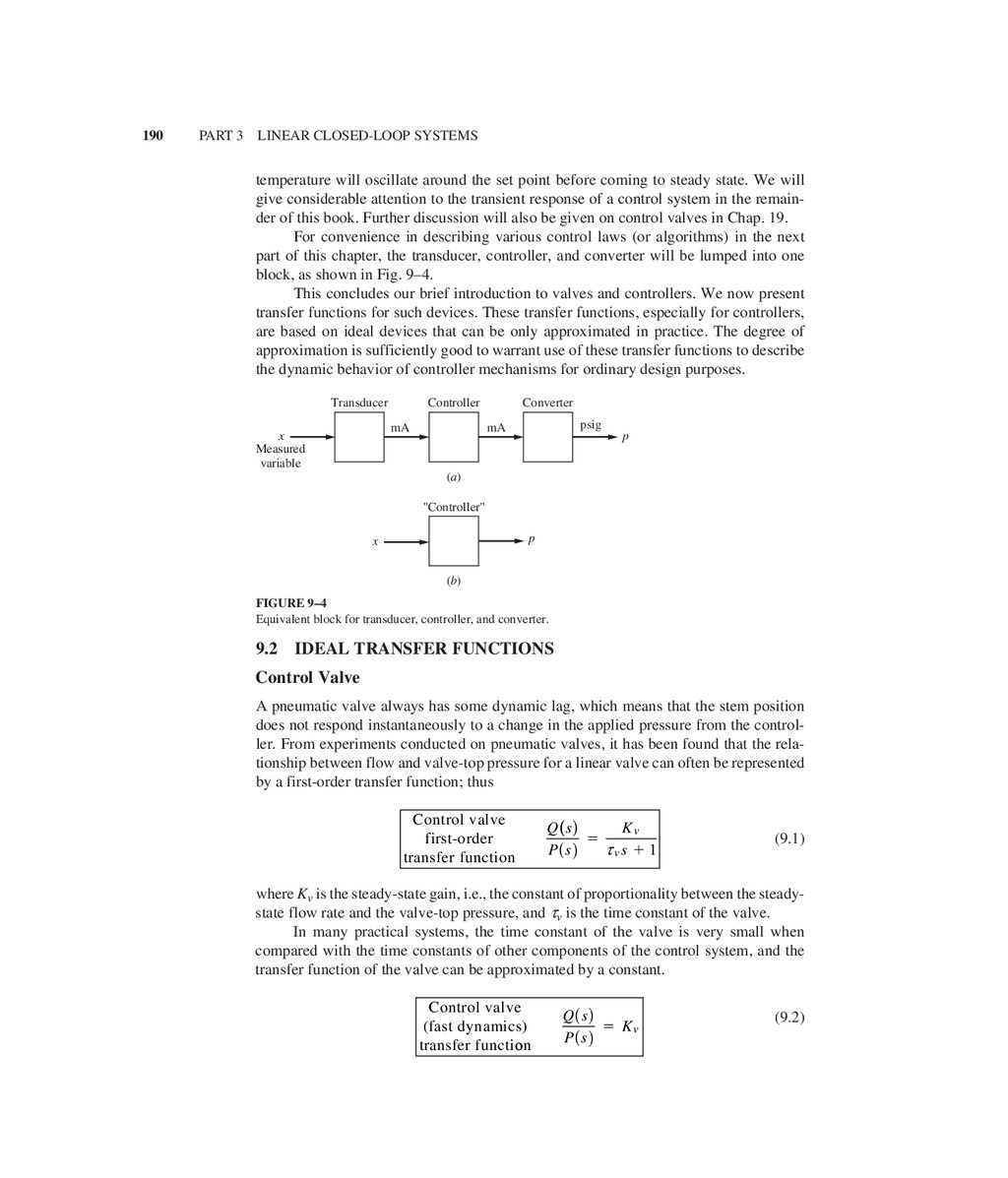
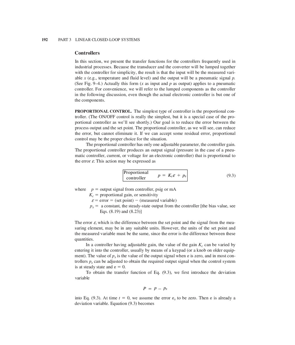
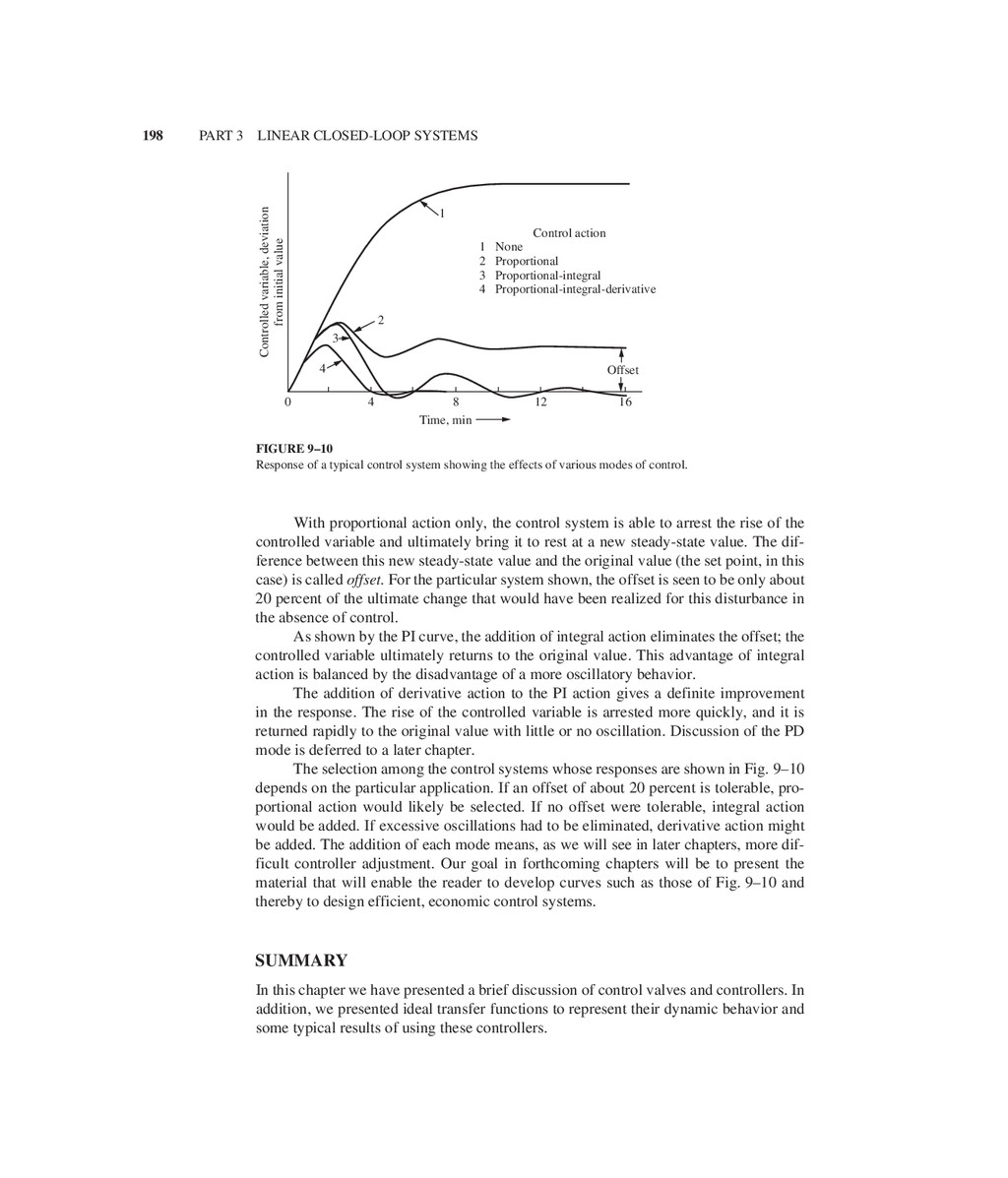
    we present the transfer functions for the controllers frequently used in industrial processes. Because the transducer and the converter will be lumped together with the controller for simplicity, the result is that the input will be the measured vari- able x (e.g., temperature and fluid level) and the output will be a pneumatic signal p. (See Fig. 9–4 .) Actually this form ( x as input and p as output) applies to a pneumatic controller. For convenience, we will refer to the lumped components as the controller in the following discussion, even though the actual electronic controller is but one of the components. PROPORTIONAL CONTROL. The simplest type of controller is the proportional con- troller. (The ON/OFF control is really the simplest, but it is a special case of the pro- portional controller as we’ll see shortly.) Our goal is to reduce the error between the process output and the set point. The proportional controller, as we will see, can reduce the error, but cannot eliminate it. If we can accept some residual error, proportional control may be the proper choice for the situation. The proportional controller has only one adjustable parameter, the controller gain. The proportional controller produces an output signal (pressure in the case of a pneu- matic controller, current, or voltage for an electronic controller) that is proportional to the error e. This action may be expressed as Proportional controller p K p c s ϭ ϩ e (9.3) where p ϭ output signal from controller, psig or mA K c ϭ proportional gain, or sensitivity e ϭ error ϭ (set point) Ϫ (measured variable) p s ϭ a constant, the steady-state output from the controller [the bias value, see Eqs. (8.19) and (8.23)] The error e, which is the difference between the set point and the signal from the mea- suring element, may be in any suitable units. However, the units of the set point and the measured variable must be the same, since the error is the difference between these quantities. In a controller having adjustable gain, the value of the gain K c can be varied by entering it into the controller, usually by means of a keypad (or a knob on older equip- ment). The value of p s is the value of the output signal when e is zero, and in most con- trollers p s can be adjusted to obtain the required output signal when the control system is at steady state and e ϭ 0. To obtain the transfer function of Eq. (9.3), we first introduce the deviation variable P p ps ϭ Ϫ into Eq. (9.3). At time t ϭ 0, we assume the error e s to be zero. Then e is already a deviation variable. Equation (9.3) becomes
  8. CHAPTER 9 CONTROLLERS AND FINAL CONTROL ELEMENTS 193 P t

    K t c ( ) ( ) ϭ e (9.4) Taking the transform of Eq. (9.4) gives the transfer function of an ideal proportional controller. Proportional controller transfer function P s ( ) ) ( ) e s Kc ϭ (9.5) The actual behavior of a proportional controller is depicted in Fig. 9–6 . The controller output will saturate (level out) at p max ϭ 15 psig or 20 mA at the upper end and at p min ϭ 3 psig or 4 mA at the lower end of the output. The ideal transfer func- tion Eq. (9.5) does not predict this saturation phenomenon. The next example will help to clarify the concept of controller gain. Example 9.1. A pneumatic proportional controller is used in the process shown in Fig. 9–2 to control the cold stream outlet temperature within the range of 60 to 120 Њ F. The controller gain is adjusted so that the output pressure goes from 3 psig (valve fully closed) to 15 psig (valve fully open) as the measured temperature goes from 71 to 75 Њ F with the set point held constant. Find the controller gain K c . Gain psig psig F F psi/ F ϭ ϭ Ϫ Њ Ϫ Њ ϭ Њ ∆ ∆ p e 15 3 75 71 3 Now assume that the gain of the controller is changed to 0.4 psi/ Њ F. Find the error in temperature that will cause the control valve to go from fully closed to fully open. ∆ ∆ T p ϭ ϭ Њ ϭ Њ gain psi psi/ F F 12 0 4 30 . FIGURE 9–6 Proportional controller output as a function of error input to the controller. (a) Ideal behavior; (b) actual behavior. (a) (b) p 0 ε ε 0 ps = bias value slope = Kc Proportional controller—Ideal behavior Saturation p 0 0 ps = bias value Proportional controller—actual behavior pmin Saturation pmax
  9. 194 PART 3 LINEAR CLOSED-LOOP SYSTEMS At this level of

    gain, the valve will be fully open if the error signal reaches 30 Њ F. The gain K c has the units of psi per unit of measured variable. [Regarding the units on controller gain, if the actual controller of Fig. 9–4 is considered, both the input and the output units are in milliamperes. In this case the gain will be dimensionless (i.e., mA/mA).] ON/OFF CONTROL. A special case of proportional control is on/off control. If the gain K c is made very high, the valve will move from one extreme position to the other if the process deviates only slightly from the set point. This very sensitive action is called on/ off action because the valve is either fully open (on) or fully closed (off); i.e., the valve acts as a switch. This is a very simple controller and is exemplified by the thermostat used in a home-heating system. In practice, a dead band is inserted into the controller. With a dead band, the error reaches some finite positive value before the controller “turns on.” Conversely, the error must fall to some finite negative value before the controller “turns off.” This behavior is shown in Fig. 9–7 . Expanding the width of the dead band makes the controller less sensitive to noise and prevents the phenomenon of chattering, where the controller will rapidly cycle on and off as the error fluctuates about zero. Chattering is detrimental to equipment performance. For various reasons, it is often desirable to add other modes of control to the basic proportional action. These modes, integral and derivative action, are discussed below with the objective of obtaining the ideal transfer functions of the expanded controllers. The reasons for introducing these modes will be discussed briefly at the end of this chapter and in greater detail in later chapters. PROPORTIONAL-INTEGRAL (PI) CONTROL. If we cannot tolerate any residual error, we will have to introduce an additional control mode: integral control. If we add integral control to our proportional controller, we have what is termed PI, or proportional-integral FIGURE 9–7 Output from on/off controller as a function of error input to the controller. (a) Ideal on/off controller; (b) on/off controller with dead band. (b) (a) p 0 0 On/off controller with dead band p 0 0 Ideal on/off controller pmax pmax pmin pmin Slope = Kc = infinite Dead band ε ε
  10. CHAPTER 9 CONTROLLERS AND FINAL CONTROL ELEMENTS 195 control. The

    integral mode ultimately drives the error to zero. This controller has two adjustable parameters for which we select values, the gain and the integral time. Thus it is a bit more complicated than a proportional controller, but in exchange for the addi- tional complexity, we reap the advantage of no error at steady state. PI control is described by the relationship Proportional-integral controller p K K c c I ϭ ϩ e t e edt ps + ∫ 0 t (9.6) where K c ϭ proportional gain t I ϭ integral time, min p s ϭ constant (the bias value) In this case, we have added to the proportional action term K c e another term that is proportional to the integral of the error. The values of K c and t I are both adjustable. To visualize the response of this controller, consider the response to a unit-step change in error, as shown in Fig. 9–8 . This unit-step response is most directly obtained by inserting e ϭ 1 into Eq. (9.6), which yields p t K K t p c c I s ( ) ϭ ϩ ϩ t (9.7) τI Kc Kc ps p t 0 0 1 } FIGURE 9–8 Response of a PI controller to a unit-step change in error. Notice that p changes suddenly by an amount K c and then changes linearly with time at a rate K c / t I . To obtain the transfer function of Eq. (9.6), we again introduce the deviation vari- able P ϭ p Ϫ p s into Eq. (9.6) and then take the transform to obtain Proportional-integral controller transfer func ction P s s K s c I ( ) ( )       e t ϭ ϩ 1 1 (9.8)
  11. 196 PART 3 LINEAR CLOSED-LOOP SYSTEMS Some manufacturers prefer to

    use the term reset rate, which is defined as the reciprocal of t I . The integral adjustment on a controller may be denoted by integral time or reset rate (carefully check the specific controller to be sure which value to enter). The cali- bration of the proportional and integral action is often checked by observing the jump and slope of a step response, as shown in Fig. 9–8 . PROPORTIONAL-DERIVATIVE (PD) CONTROL. Derivative control is another mode that can be added to our proportional or proportional-integral controllers. It acts upon the derivative of the error, so it is most active when the error is changing rapidly. It serves to reduce process oscillations. This mode of control may be represented by Proportional-derivative controller p K K c c D ϭ ϩ e t d d dt ps e ϩ (9.9) where K c ϭ proportional gain t D ϭ derivative time, min p s ϭ constant (bias value) In this case, we have added to the proportional term another term K c t D d e/ dt, which is proportional to the derivative of the error. The values of K c and t D are both adjustable. Other terms that are used to describe the derivative action are rate control and anticipa- tory control. The action of this controller can be visualized by considering the response to a linear change in error as shown in Fig. 9–9 . FIGURE 9–9 Response of a PD controller to a ramp input in error. AKc Derivative alone Proportional alone A 1 1 ps p t 0 0 } AKc D This response is obtained by introducing the linear function e ( t ) ϭ At into Eq. (9.9) to obtain p t AK t AK p c c D s ( ) ϭ ϩ ϩ t Notice that p changes suddenly by an amount AK c t D as a result of the derivative action and then changes linearly at a rate AK c . The effect of derivative action in this case is to
  12. CHAPTER 9 CONTROLLERS AND FINAL CONTROL ELEMENTS 197 anticipate the

    linear change in error by adding output AK c t D to the proportional action. The controller is taking preemptive action to counter the anticipated change in the error that it predicted from the slope of the error versus time curve. To obtain the transfer function from Eq. (9.9), we introduce the deviation variable P ϭ p Ϫ p s and then take the transform to obtain Proportional-derivative controller transfer fu unction P s s K s c D ( ) ( ) ( ) e t ϭ ϩ 1 (9.10) PROPORTIONAL-INTEGRAL-DERIVATIVE (PID) CONTROL. This mode of control is a combination of the previous modes and is given by the expression Proportional-integral-derivative controller p ϭ ϭ ϩ ϩ ϩ K K d dt K dt p c c D c I t s e t e t e 0 ∫ (9.11) In this case, all three values K c , t D , and tI can be adjusted in the controller. The transfer function for this controller can be obtained from the Laplace transform of Eq. (9.11); thus Proportional-integral-derivative controller tr ransfer function P s s K s s c D I ( ) ( )      e t t ϭ ϩ ϩ 1 1   (9.12) Derivative action is based on how rapidly the error is changing, not the magni- tude of the error or how long the error has persisted. It is based on the slope of the error versus time curve at any instant in time. Therefore, a rapidly changing error signal will induce a large derivative response. “Noisy” error signals cause significant problems for derivative action because of the rapidly changing slope of the error caused by noise. Derivative control should be avoided in these situations unless the error signal can be filtered to remove the noise. Motivation for Addition of Integral and Derivative Control Modes Having introduced ideal transfer functions for integral and derivative modes of con- trol, we now wish to indicate the practical motivation for use of these modes. The curves of Fig. 9–10 show the behavior of a typical feedback control system using different kinds of control when it is subjected to a permanent disturbance. This may be visualized in terms of the stirred-tank temperature control system of Chap. 8 after a step change in T i . The value of the controlled variable is seen to rise at time zero owing to the disturbance. With no control, this variable continues to rise to a new steady-state value. With control, after some time the control system begins to take action to try to maintain the controlled variable close to the value that existed before the disturbance occurred.
  13. 198 PART 3 LINEAR CLOSED-LOOP SYSTEMS With proportional action only,

    the control system is able to arrest the rise of the controlled variable and ultimately bring it to rest at a new steady-state value. The dif- ference between this new steady-state value and the original value (the set point, in this case) is called offset. For the particular system shown, the offset is seen to be only about 20 percent of the ultimate change that would have been realized for this disturbance in the absence of control. As shown by the PI curve, the addition of integral action eliminates the offset; the controlled variable ultimately returns to the original value. This advantage of integral action is balanced by the disadvantage of a more oscillatory behavior. The addition of derivative action to the PI action gives a definite improvement in the response. The rise of the controlled variable is arrested more quickly, and it is returned rapidly to the original value with little or no oscillation. Discussion of the PD mode is deferred to a later chapter. The selection among the control systems whose responses are shown in Fig. 9–10 depends on the particular application. If an offset of about 20 percent is tolerable, pro- portional action would likely be selected. If no offset were tolerable, integral action would be added. If excessive oscillations had to be eliminated, derivative action might be added. The addition of each mode means, as we will see in later chapters, more dif- ficult controller adjustment. Our goal in forthcoming chapters will be to present the material that will enable the reader to develop curves such as those of Fig. 9–10 and thereby to design efficient, economic control systems. SUMMARY In this chapter we have presented a brief discussion of control valves and controllers. In addition, we presented ideal transfer functions to represent their dynamic behavior and some typical results of using these controllers. Control action Offset None Proportional Proportional-integral Proportional-integral-derivative 1 2 3 4 1 2 3 4 0 Controlled variable, deviation from initial value 16 12 8 Time, min 4 FIGURE 9–10 Response of a typical control system showing the effects of various modes of control.
  14. CHAPTER 9 CONTROLLERS AND FINAL CONTROL ELEMENTS 199 The ideal

    transfer functions actually describe the action of many types of con- trollers, including pneumatic, electronic, computer-based, hydraulic, mechanical, and electrical systems. Hence, the mathematical analyses of control systems to be presented in later chapters, which are based upon first- and second-order systems, transportation lags, and ideal controllers, generalize to many branches of the control field. After study- ing this text on process control, the reader should be able to apply the knowledge to, e.g., problems in mechanical control systems. All that is required is a preliminary study of the physical nature of the systems involved. PROBLEMS 9.1. A pneumatic PI temperature controller has an output pressure of 10 psig when the set point and process temperature coincide. The set point is suddenly increased by 10 Њ F (i.e., a step change in error is introduced), and the following data are obtained: Time, s psig 0Ϫ 10 0ϩ 8 20 7 60 5 90 3.5 Determine the actual gain (psig per degree Fahrenheit) and the integral time. 9.2. A unit-step change in error is introduced into a PID controller. If K c ϭ 10, t I ϭ 1, and t D ϭ 0.5, plot the response of the controller P ( t ). 9.3. An ideal PD controller has the transfer function P K s c D e t ϭ ϩ 1 ( ) An actual PD controller had the transfer function P K s s c D D e t t b ϭ ϩ ϩ 1 1 ( ) / where b is a large constant in an industrial controller. If a unit-step change in error is introduced into a controller having the second transfer function, show that P t K Ae c t D ( ) ( ) ϭ ϩ Ϫ 1 b t / where A is a function of b which you are to determine. For b ϭ 5 and K c ϭ 0.5, plot P ( t ) versus t / t D . As b → ϱ , show that the unit-step response approaches that for the ideal controller. 9.4. A PID temperature controller is at steady state with an output pressure of 9 psig. The set point and process temperature are initially the same. At time t ϭ 0, the set point is increased at the rate of 0.5 Њ F/min. The motion of the set point is in the direction of lower temperatures. If the current settings are
  15. 200 PART 3 LINEAR CLOSED-LOOP SYSTEMS Kc i D ϭ

    Њ ϭ ϭ 2 1 25 0 4 psig/ F min min t t . . plot the output pressure versus time. 9.5. The input e to a PI controller is shown in Fig. P9–5 . Plot the output of the controller if K c ϭ 2 and t I ϭ 0.50 min. 1 0.5 0 0 1 2 3 4 t, min −0.5 −1 ε FIGURE P9–5 9.6. A PI controller has the transfer function G s s c ϭ ϩ 5 10 Determine the values of K c and t I . 9.7. Dye for our new line of blue jeans is being blended in a mixing tank. The desired color of blue is produced using a concentration of 1500 ppm blue dye, with a minimum acceptable con- centration of 1400 ppm. At 9 A.M. today the dye injector plugged, and the dye flow was inter- rupted for 10 min, until we realized the problem and unclogged the nozzle. see Fig. P9–7 . 20 gal/min Concentrated dye injector 20 gal/min aqueous dye for jeans (1500 ppm blue dye) V = 100 gal Water Color analyzer PI FIGURE P9–7 Plot the controller ouput from 9 A.M. to 9:10 A.M. The steady-state controller output (the bias value) is 8 psig. Does the controller output saturate (output range is 3 to 15 psig)? If so, at what time does it occur? The controller is a PI controller with K c ϭ 0.001 psig/ppm and t I ϭ 1 min.
  16. 201 CHAPTER 9 CAPSULE SUMMARY CONTROL VALVES Two basic types

    of control valves are air-to-close and air-to-open. The air pres- sure (pneumatic) signal is usually 3 to 15 psig. The dynamics of the valves are adequately modeled as first-order sys- tems. The time constant is on the order of 1 s. Controller type Time domain model Transfer function Proportional (P) p ϭ Kc eϩ ps P s s Kc ( ) ( ) e ϭ Proportional-integral (PI) p K K dt p c c I t s ϭ ϩ ϩ e t e 0 ∫ P s s K s c I ( ) ( )       e t ϭ ϩ 1 1 Proportional-derivative (PD) p K K d dt p c c D s ϭ ϩ ϩ e t e P s s K s c D ( ) ( ) ( ) e t ϭ ϩ 1 Proportional-integral- derivative (PID) p K K d dt K dt p c c D c I t s ϭ ϩ ϩ ϩ e t e t e 0 ∫ P s s K s s c D I ( ) ( )       e t t ϭ ϩ ϩ 1 1 CONTROLLERS Control valuve first-order transfer function Q s s P s K s v v ( ) ( ) ϭ ϩ t 1 Control valuve first-order transfer function Q s s P s K s v v ( ) ( ) ϭ ϩ t 1 Control valve fast dynamics transfer functi ( ) o on Q s P s Kv ( ) ( ) ϭ Control valve fast dynamics transfer functi ( ) o on Q s P s Kv ( ) ( ) ϭ Air Motor p Valve Stem Air-to-close Plug Air Motor p Valve Stem Air-to-open (b) (a) Plug