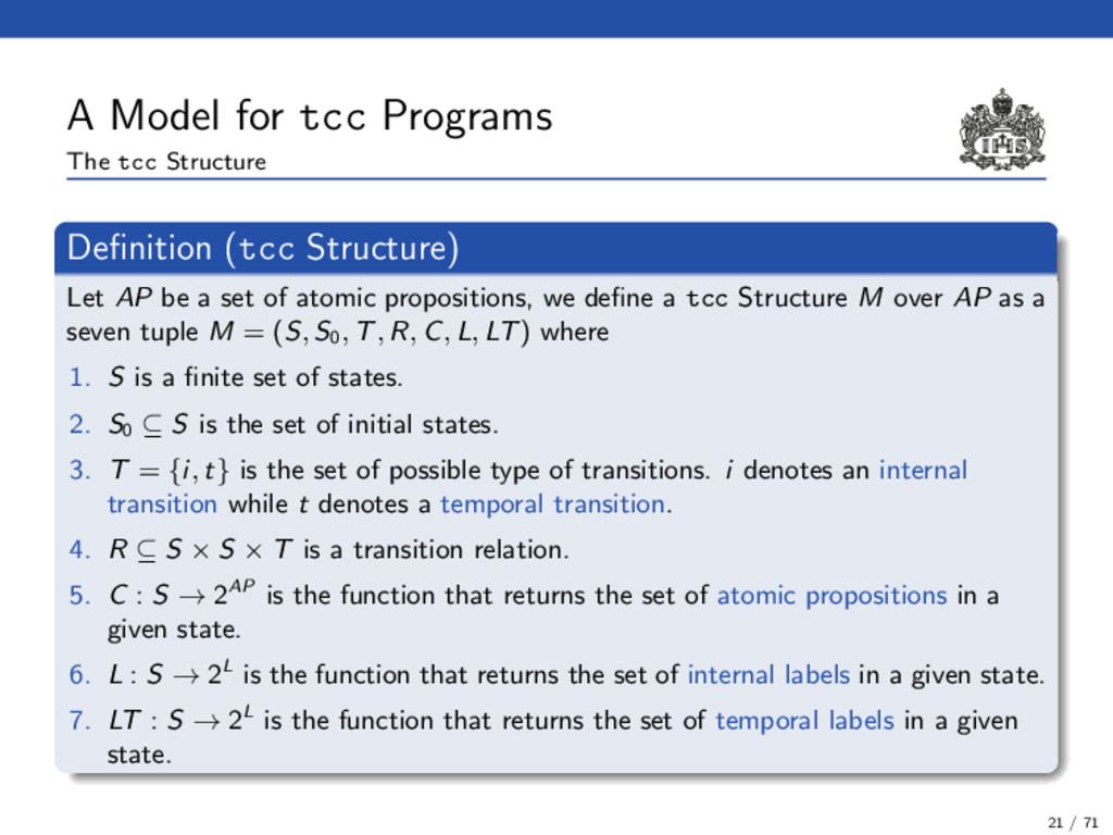
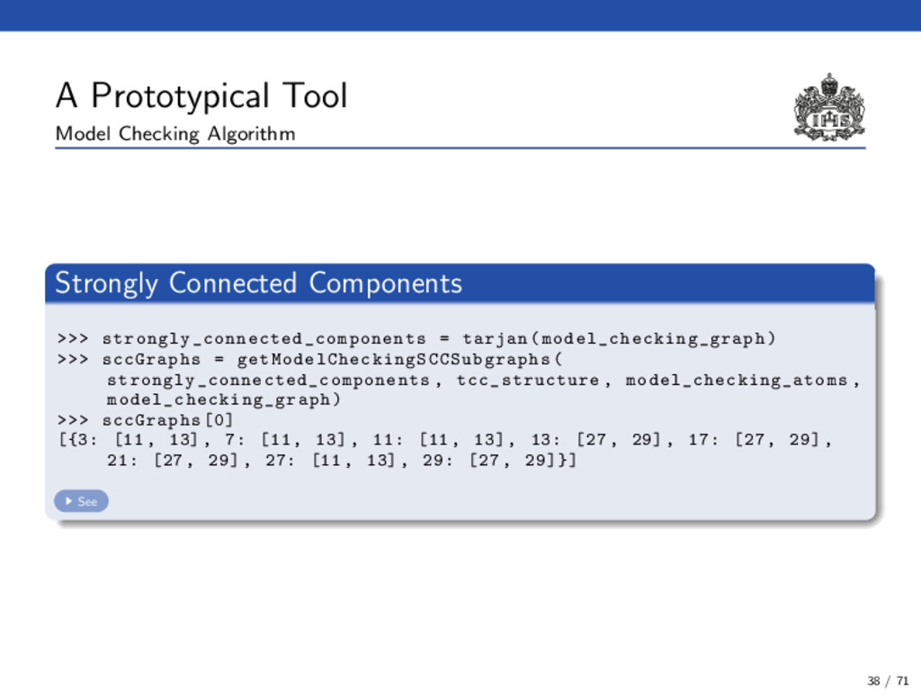
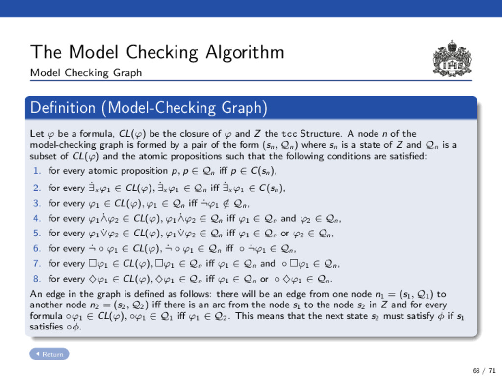
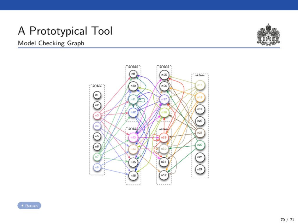
for con- currency where agents interact with one another by adding (telling) and reading (asking) information represented as constraints in a shared medium (global store). • The type of constraints and the entailment relation is given by a Constraint System (e.g. x > 42 |= x > 0). 3 / 71
by adding temporal constructs for modeling timed and reactive systems. • Formal verification plays an important role in detecting errors in concurrent systems. The presence of a system failure in air traffic control systems, medical instruments, aircrafts or in general, reactives systems could be catastrophic. (a) Therac-25 (b) Ariane-5 Figure: Some disasters 4 / 71
techniques since the model does not provide automatic formal verification tools. • Problems: ◦ Difficult ◦ Error prone ◦ Experts are required. • Hubert Garavel [Gar08]: “...The research agenda for theoretical concur- rency should therefore address the design of efficient algorithms for trans- lating and verifying formal specifications of concurrent systems”. 5 / 71
a finite-state model of a system and a formal property, systematically checks whether this property holds for (a given state in) that model [CGP99]. • Advantages ◦ Formal technique. ◦ Fully-automatic. ◦ Experts are not required. ◦ Counterexample. • Drawback: ◦ State-space explosion problem. 6 / 71
Model Checking Satisfied Violated + Counterexample ntcc LTL tcc Structure Classical approach and prototype Our approach: A model checking algorithm based on the work of Falaschi and Villanueva [FV06]. 8 / 71
a tcc program. • An algorithm for constructing the model from the tcc specification. • A method for reducing the size of a model. • A model checking algorithm for verifying tcc programs. • A prototype of the model checking algorithm. 9 / 71
3 A Model for tcc Programs 4 A Logic for the Specification of Properties 5 The Model Checking Algorithm 6 A Prototypical Tool 7 Application 8 Concluding Remarks 10 / 71
3 A Model for tcc Programs 4 A Logic for the Specification of Properties 5 The Model Checking Algorithm 6 A Prototypical Tool 7 Application 8 Concluding Remarks 11 / 71
Time Unit 1 ccp Process 1. Receives a stimulus (i.e. a constraint) from the environment. 2. Computes a ccp process in the current time unit and wait for stability. 13 / 71
Time Unit 1 Resting Point Final Store 1. Receives a stimulus (i.e. a constraint) from the environment. 2. Computes a ccp process in the current time unit and wait for stability. 3. Responds with the resulting store. 13 / 71
Time Unit 1 Resting Point Final Store Residual Process Store Time Unit 2 1. Receives a stimulus (i.e. a constraint) from the environment. 2. Computes a ccp process in the current time unit and wait for stability. 3. Responds with the resulting store. 4. Executes the residual process in the next time unit. * Note: Stores are not automatically transferred from a time unit to the next one. 13 / 71
time interval tell (c) telling information add c to the store in the current time interval now c then P asking information executes P if c can be deduced from the current store ∃x (P) hiding executes P with local x P || Q parallelism executes P and Q next P unit-delay executes P in the next time unit now c else P time-out executes P in the next time unit if c cannot be entailed now Syntax SOS 14 / 71
3 A Model for tcc Programs 4 A Logic for the Specification of Properties 5 The Model Checking Algorithm 6 A Prototypical Tool 7 Application 8 Concluding Remarks 16 / 71
System Model Model Checking Satisfied Violated + Counterexample System Model: Models of systems describe the behavior of systems in a formal way. They are mostly expressed using transition systems. 17 / 71
System Model Model Checking Satisfied Violated + Counterexample Property Specification: Properties should be described in a precise and unambiguous manner. Temporal logic is typically used to express properties. 17 / 71
System Model Model Checking Satisfied Violated + Counterexample Model Checking: Algorithm which checks the validity of the property in all states of the system model. 17 / 71
3 A Model for tcc Programs 4 A Logic for the Specification of Properties 5 The Model Checking Algorithm 6 A Prototypical Tool 7 Application 8 Concluding Remarks 18 / 71
process consists in assigning a different label to each occur- rence of an agent in the program. • Labels provide an unique identification for agents in order to know the point of execution of the program during the construction of the model. Example {lp0 }p():: {l||1 }({lnowp2 }now (in=true) then {lnext3 }next({ltell4 }tell(x=2)) || {l||5 }({lnown6 }now (in=true) else {ltell7 }tell(x=1) || {lnext8 }next({lp9 }p()))) Definition 19 / 71
Structure is a graph structure which allows to model the behavior of a tcc specification. • It is a variant of a Kripke Structure. current store internal labels temporal labels (a) tcc state Internal Transition Temporal Transition (b) Transitions Figure: Components of a tcc Structure Definition 20 / 71
Structure) Let AP be a set of atomic propositions, we define a tcc Structure M over AP as a seven tuple M = (S, S0, T, R, C, L, LT) where 1. S is a finite set of states. 2. S0 ⊆ S is the set of initial states. 3. T = {i, t} is the set of possible type of transitions. i denotes an internal transition while t denotes a temporal transition. 4. R ⊆ S × S × T is a transition relation. 5. C : S → 2AP is the function that returns the set of atomic propositions in a given state. 6. L : S → 2L is the function that returns the set of internal labels in a given state. 7. LT : S → 2L is the function that returns the set of temporal labels in a given state. 21 / 71
Transitions are described according to the operational rules of each tcc process. • For each different declaration we construct a tcc Structure. • Each state is composed of labels associated with agents that can be executed in a step of the construction process. • Each label can be active or disable. • The labels associated with temporal agents cannot be executed before all the labels associated with normal agents are executed. Algorithm 22 / 71
States: 6 tell4, p9 in=true 7 tell4, p9 13 tell4, p9 x=2, in=true • Reduction of states is necessary to decrease the state explosion problem. • The store on the quiescent point is defined as the output of the computation. 24 / 71
3 A Model for tcc Programs 4 A Logic for the Specification of Properties 5 The Model Checking Algorithm 6 A Prototypical Tool 7 Application 8 Concluding Remarks 26 / 71
• Linear temporal logic (LTL) named CLTL for reasoning about ntcc processes. • It expresses properties over sequences of constraints. • ntcc is an extension of tcc. Definition (CLTL Syntax) The formulae F, G, . . . ∈ F are built from constraints c ∈ C in the underlying constraint system by F, G, . . . := c | ˙ true | ˙ false | F ˙ ∧ G | F ˙ ∨ G | ˙ ¬F | ˙ ∃x F | ◦ F | F | ♦F Semantics 27 / 71
3 A Model for tcc Programs 4 A Logic for the Specification of Properties 5 The Model Checking Algorithm 6 A Prototypical Tool 7 Application 8 Concluding Remarks 28 / 71
LTL model checking problem [CGP99, MP95, LP85]. • To prove that a property is satisfied, it is possible to prove that there is no path in the model checking graph satisfying the negation of the formula. 29 / 71
graph G, we define a Strongly Connected Component (SCC) S as a maximal subgraph of G such that for every two distinct nodes A, B ∈ S, there exists a path from A to B that passes through nodes of S. We say that S is transient if it consists of a single node that is not connected to itself. Definition (Self-fulfilling SCC) Given a model-checking graph G, a self-fulfilling strongly connected component C is defined as a non-transient strongly connected component in G which satisfies that for every node n in C and for every ♦φ ∈ Qn there exists a node m in C such that φ ∈ Qm . 30 / 71
checking graph using the negation of φ (i.e. ¬φ). Definition ◦ First of all, we have to compute the closure CL(¬φ). This closure is reminiscent to the Fisher Ladner’s one [MP95, FL79]. Definition 31 / 71
checking graph using the negation of φ (i.e. ¬φ). Definition ◦ First of all, we have to compute the closure CL(¬φ). This closure is reminiscent to the Fisher Ladner’s one [MP95, FL79]. Definition 2. To look for a sequence such that starting from an initial node of the graph that satisfies the negation of φ, it reaches a self-fulfilling strongly connected component. 31 / 71
checking graph using the negation of φ (i.e. ¬φ). Definition ◦ First of all, we have to compute the closure CL(¬φ). This closure is reminiscent to the Fisher Ladner’s one [MP95, FL79]. Definition 2. To look for a sequence such that starting from an initial node of the graph that satisfies the negation of φ, it reaches a self-fulfilling strongly connected component. 3. If we find a self-fulfilling SCC in the graph, then the system satisfies the property represented by the negated formula (i.e. the model does not satisfy the property). 31 / 71
3 A Model for tcc Programs 4 A Logic for the Specification of Properties 5 The Model Checking Algorithm 6 A Prototypical Tool 7 Application 8 Concluding Remarks 32 / 71
3 A Model for tcc Programs 4 A Logic for the Specification of Properties 5 The Model Checking Algorithm 6 A Prototypical Tool 7 Application 8 Concluding Remarks 41 / 71
technique for verifying finite-state reactive systems, and in particular, digital systems [Kot08a] (e.g. Traffic light controller [BCDM86, Swa97], radar jammer [CEP03], sequence detec- tor [KK09], binary comparator [Kot08b]). • The coffee machine provides the user with a cup of coffee or a cup of hot water (for tea), given that the consumer has inserted the required amount of money. Coffee 10 5 Tea 42 / 71
the digital system using tcc. • To create the model (tcc Structure) of the system. • To specify the properties to be verified. • Use the model checking algorithm to determine whether the model satisfies the property. 43 / 71
3 A Model for tcc Programs 4 A Logic for the Specification of Properties 5 The Model Checking Algorithm 6 A Prototypical Tool 7 Application 8 Concluding Remarks 44 / 71
for tcc, an automated formal verification tool. • Model of the system: ◦ Structure (tcc Structure) to model the behavior of a tcc system. ◦ Algorithm to construct the tcc Structure from the tcc specification. ◦ Method to simplify the model. • Temporal logic to specify properties of tcc systems. • Algorithm to determine whether the model of the system satisfies a formula. • Prototype of the model checking algorithm. 45 / 71
construction algorithm. • Automatic tool for constructing the model of the system. • Symbolic and abstract techniques for reducing the state explosion problem. • ntcc model checking. • Prototype improvement (e.g. compute automatically the negated form of the formulas). 46 / 71
Dill, and Bud Mishra. Automatic Verification of Sequential Circuits Using Temporal Logic. IEEE Transactions on Computers, C-35(12):1035–1044, 1986. Luis Alejandro Cort´ es, Petru Eles, and Zebo Peng. Modeling and Formal Verification of Embedded Systems Based On a Petri Net Representation. Journal of Systems Architecture, 49:571–598, 2003. Edmund M. Clarke, Orna Grumberg, and Doron A. Peled. Model Checking. MIT Press, Cambridge, 1999. Michael J. Fischer and Richard E. Ladner. Propositional Dynamic Logic of Regular Programs. Journal of Computer and System Sciences, 18(2):194–211, 1979. 48 / 71
Timed Concurrent Constraint Programs. Theory and Practice of Logic Programming, 6(3):265–300, 2006. Hubert Garavel. Reflections on the Future of Concurrency Theory in General and Process Calculi in Particular. In Proceedings of LIX Colloquium on Emergent Trends in Concurrency Theory, volume 209 of Electronic Notes in Theoretical Computer Science, pages 149–164. Elsevier, 2008. C. A. R. Hoare. Communicating Sequential Processes. Prentice Hall, 1985. 49 / 71
of Model Checking to the Verification of Digital Systems. Acta Electrotechnica et Informatica, 9(2):30–37, 2009. Daniela Kotmanov´ a. Temporal Logic in Verification of Digital Circuits. Journal of Electrical Engineering, 59(1):14–22, 2008. Daniela Kotmanov´ a. Temporal Logic in Verification of Digital Circuits. Journal of Electrical Engineering, 59(1):14–22, 2008. 50 / 71
State Concurrent Programs Satisfy their Linear Specification. In Proceedings of the 12th ACM SIGACT-SIGPLAN Symposium on Principles of Programming Languages, pages 97–107, New York, NY, USA, 1985. ACM Press. Robin Milner. Communication and Concurrency. International Series in Computer Science. Prentice Hall, 1989. Robin Milner. Communicating and Mobile Systems: the Pi-Calculus. Cambridge University Press, 1999. 51 / 71
Reactive Systems: Safety. Springer-Verlag New York, Inc., 1995. Vijay A. Saraswat. Concurrent Constraint Programming. The MIT Press, 1993. Vijay A. Saraswat, Radha Jagadeesan, and Vineet Gupta. Programming in Timed Concurrent Constraint Languages. In Constraint Programming: Proceedings 1993, NATO Advanced Science Institute Series, pages 361–410, Berlin, 1994. Springer-Verlag. Davide Sangiorgi and David Walker. The Pi-Calculus: A Theory of Mobile Processes. Cambridge University Press, 2003. 52 / 71
(Tell) | now c then A (Timed Positive Ask) | now c else A (Timed Negative Ask) | next A (Unit Delay) | abort (Abort) | skip (Skip) | A || A (Parallel Composition) | ∃x(A) (Hiding) | g (Procedure Call) (Procedure Calls) g ::= p(t1, . . . , tn) (Declarations) D ::= g :: A (Definition) | D.D (Conjunction) (Programs) P ::= D.A Return 54 / 71
The binary relation → on configurations is the least relation satisfying the rules : (?, skip) → ? (?, abort) → abort (?, A || B) → (?, A, B) (?, ∃x(A)) → (?, A[y/x]) (y not free in ?) (?, p(t1, . . . , tn)) → (?, A[x1 → t1, . . . , xn → tn]) σ(?) c (?, now c then A) → (?, A) σ(?) c (?, now c else B) → ? Axioms for . The binary relation is the least relation satisfying the single rule : ∆, {now ci else Ai | i < n} ∆, {now ci else Ai | i < n}, {next Bj | j < m} {Ai | i < n}, {Bj | j < m} Return 55 / 71
a tcc specification, the labeled version Pl of P is defined as follows. The subindex k ∈ N corresponds to the number of labels introduced up to a given point. When the labeling process starts, k = 0 and each time that we introduce a new label, k is incremented by one. • If P = tell c then Pl = {ltellk } tell c. • If P = now c then A then Pl = {lnowpk } now c then Al . • If P = now c else A then Pl = {lnownk } now c else Al . • If P = next A then Pl = {lnextk } next Al . • If P = skip then Pl = {lskipk } skip. • If P = A || B then Pl = {l|| k } (Al || Bl ). • If P = p(t1, . . . , tn ) then Pl = {lpk } p(t1, . . . , tn ). Return 56 / 71
State) Let AP be the atomic propositions in the tcc syntax and L be the set of all labels generated during the labeling process described above. We define the set of states as S ⊆ 2AP × 2L. Definition (Equivalent States) Given two tcc states s and s , we say that two states are equivalent if 1. the set of labels of s and s coincide, and 2. there exists a renaming γ of variables of the constraints in s which makes them syntactically identical to the set of constraints of s . Return 57 / 71
procedure consists in locating an active label and perform the actions associated with such agent. The process is performed while there are active labels. When we reach a state where there is no active labels (quiescent point) we have to pass to the next time unit, and then we continue with the procedure. We represent this passage in our graph as follows: 1. Introduce a new node s related with s by a temporal transition. The state s is a state where there is no active labels. 2. We introduce the temporal labels of s in the labels of s . 3. The store and the temporal labels of s are empty. Return 58 / 71
S ≡ {ltellk } tell c. The new information c is added to the store in the current time. We translate this behavior to our graph structure as follows: 1. Add a new node s related with the node s from which the agent is execute. 2. The store of s is defined as the store of s plus the constraint c (i.e. C(s ) = C(s) ∧ c). 3. The internal labels of s are obtained from those of s by removing {ltellk } (i.e. L(s ) = L(s)\{ltellk }). 4. The temporal labels of s are the same as s (i.e. LT(s ) = LT(s)). Return 59 / 71
S ≡ {l|| k } (Al || Bl ). The agents A and B are executed in parallel. We translate this behavior to our graph structure as follows: 1. Introduce a new node s related with the node s from which the agent is execute. 2. The internal labels of s are obtained from those of s by adding Al and Bl , and removing {l|| k }. Notice that this corresponds to a concurrent semantics rather than an interleaving interpretation of the parallel operator. 3. The store and the temporal labels of s are the same as s. Return 60 / 71
Positive Ask S ≡ {lnowpk } now c then Al . If the current store entails c then the agent A is executed or does nothing otherwise. Next we describe how to translate this agent to our graph. 1. Add two new nodes s1 , s2 related with the node s from which the agent is execute. This branch corresponds to the two possible behaviors. 2. The store of s1 is defined as the union of the store of s and the constraint c. 3. The store of s2 is defined as the store of s plus the absence of the constraint c (i.e. C(s2 ) = C(s) ∧ ∼ c). 4. The internal labels of s1 are obtained from those of s by adding Al and removing {lnowpk }. 5. The internal labels of s2 are the same as s. 6. The temporal labels of s1 and s2 are the same as s. Return 61 / 71
S ≡ {lskipk } skip. This agent does nothing at every time instant. We translate this agent to our graph as follows: 1. Construct a new node s related with the node s from which the agent is executed. 2. The internal labels of s are obtained from those of s by removing {lskipk }. 3. The store and the temporal labels of s are the same as s. Return 62 / 71
Call S ≡ {lpk } p(t1, . . . , tn ). This operator refers to another procedure which have different labels and variables. To translate this agent to our graph we create a new node and the label associated to the first agent of p is added to the internal labels of the node. Return 63 / 71
Negative Ask S ≡ {lnownk } now c else Al . If on the quiescent point the store does not entail c then the agent A is executed in the next time instant, or does nothing otherwise. We translate this behavior to our graph as follows: 1. Introduce two new nodes s1 , s2 related with the node s from which the agent is execute. This branch corresponds to the two possible behaviors of the agent. 2. The store of s1 is defined as the union of the store of s and the constraint c. 3. The store of s2 is defined as the store of s plus the absence of the constraint c. 4. The internal labels of s1 and s2 are the same as s by removing {lnownk }. 5. The temporal labels of s1 are the same as s. 6. The temporal labels of s2 are obtained from those of s by adding Al . Return 64 / 71
Delay S ≡ {lnextk } next Al . The agent A is executed in the next time instant. We translate this agent to our graph as follows: 1. Construct a new node s related with the node s from which the agent is execute. 2. The internal labels of s are the same as s but removing {lnextk }. 3. The temporal labels of s are obtained from those of s by adding Al . 4. The store of s is the same as s. Return 65 / 71
Definition (CLTL Semantics) We say that α ∈ Cω satisfies (or that it is a model of) F in CLTL, written α CLTL F, iff α, 1 CLTL F, where: α, i CLTL ˙ true α, i CLTL ˙ false α, i CLTL c iff α(i) c α, i CLTL ˙ ¬F iff α, i CLTL F α, i CLTL F ˙ ∧ G iff α, i CLTL F and α, i CLTL G α, i CLTL F ˙ ∨ G iff α, i CLTL F or α, i CLTL G α, i CLTL ◦F iff α, i + 1 CLTL F α, i CLTL F iff for all j ≥ i α, j CLTL F α, i CLTL ♦F iff there is a j ≥ i s.t. α, j CLTL F α, i CLTL ˙ ∃x F iff there is an x-variant α of α s.t. α , i CLTL F Define F = {α | α CLTL F}. We say that F is CLTL valid iff F = Cω, and that F is CLTL satisfiable iff F = ∅. Return 66 / 71
Let ϕ be a formula, CL(ϕ) be the closure of ϕ and Z the tcc Structure. A node n of the model-checking graph is formed by a pair of the form (sn, Qn) where sn is a state of Z and Qn is a subset of CL(ϕ) and the atomic propositions such that the following conditions are satisfied: 1. for every atomic proposition p, p ∈ Qn iff p ∈ C(sn), 2. for every ˙ ∃x ϕ1 ∈ CL(ϕ), ˙ ∃x ϕ1 ∈ Qn iff ˙ ∃x ϕ1 ∈ C(sn), 3. for every ϕ1 ∈ CL(ϕ), ϕ1 ∈ Qn iff ˙ ¬ϕ1 / ∈ Qn, 4. for every ϕ1 ˙ ∧ϕ2 ∈ CL(ϕ), ϕ1 ˙ ∧ϕ2 ∈ Qn iff ϕ1 ∈ Qn and ϕ2 ∈ Qn, 5. for every ϕ1 ˙ ∨ϕ2 ∈ CL(ϕ), ϕ1 ˙ ∨ϕ2 ∈ Qn iff ϕ1 ∈ Qn or ϕ2 ∈ Qn, 6. for every ˙ ¬ ◦ ϕ1 ∈ CL(ϕ), ˙ ¬ ◦ ϕ1 ∈ Qn iff ◦ ˙ ¬ϕ1 ∈ Qn, 7. for every ϕ1 ∈ CL(ϕ), ϕ1 ∈ Qn iff ϕ1 ∈ Qn and ◦ ϕ1 ∈ Qn, 8. for every ♦ϕ1 ∈ CL(ϕ), ♦ϕ1 ∈ Qn iff ϕ1 ∈ Qn or ◦ ♦ϕ1 ∈ Qn. An edge in the graph is defined as follows: there will be an edge from one node n1 = (s1, Q1) to another node n2 = (s2, Q2) iff there is an arc from the node s1 to the node s2 in Z and for every formula ◦ϕ1 ∈ CL(ϕ), ◦ϕ1 ∈ Q1 iff ϕ1 ∈ Q2. This means that the next state s2 must satisfy φ if s1 satisfies ◦φ. Return 68 / 71