An automated computational framework for hyperelasticity

Nonlinear elasticity theory plays a fundamental role in modelling the mechanical response of many polymeric and biological materials. Such materials are capable of undergoing finite deformation, and their material response is often characterised by complex, nonlinear constitutive relationships. Because of these difficulties, predicting the response of such materials to arbitrary loads requires numerical computation (usually based on the finite element method). The steps involved in the construction of the required finite element algorithms are classical and straightforward in principle, but their application to non-trivial material models are typically tedious and error-prone. Our recent work on an automated computational framework for nonlinear elasticity, CBC.Twist, is an attempt to alleviate this problem. The framework is based on the FEniCS project, a collaborative project for the automation of computational mathematical modelling based on the finite element method.

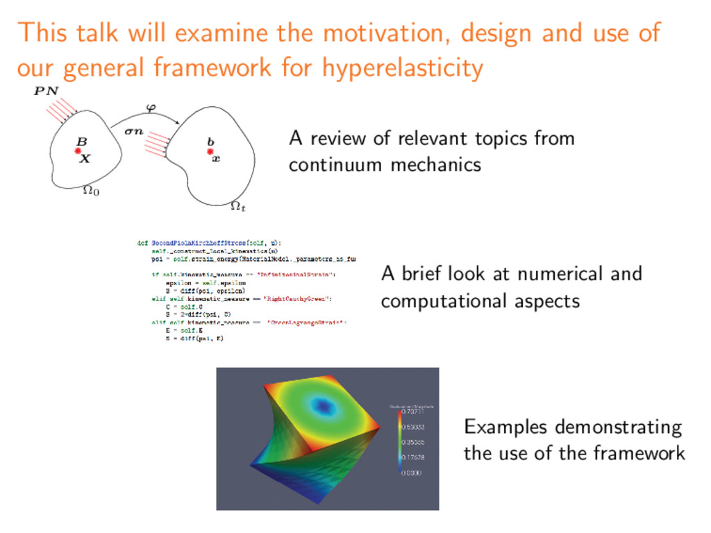
The focus of this talk will be to describe the design and implementation of the automated framework for nonlinear elasticity, as well as providing examples of its use. The goal is to allow researchers to easily pose their problems in a straightforward manner, so that they may focus on higher-level modelling questions and not be hindered by specific implementation issues. What follows is the proposed outline for the talk.

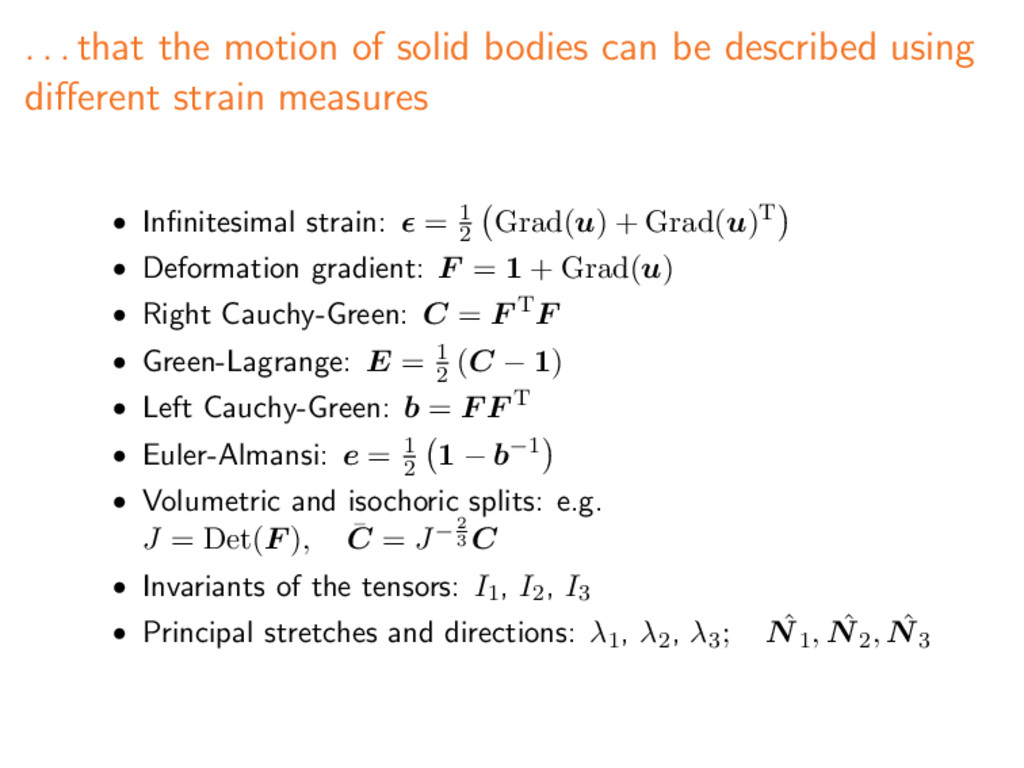
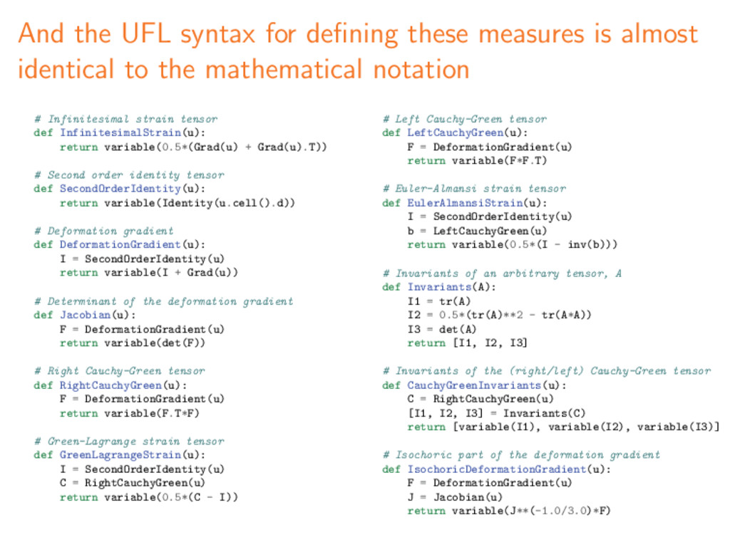
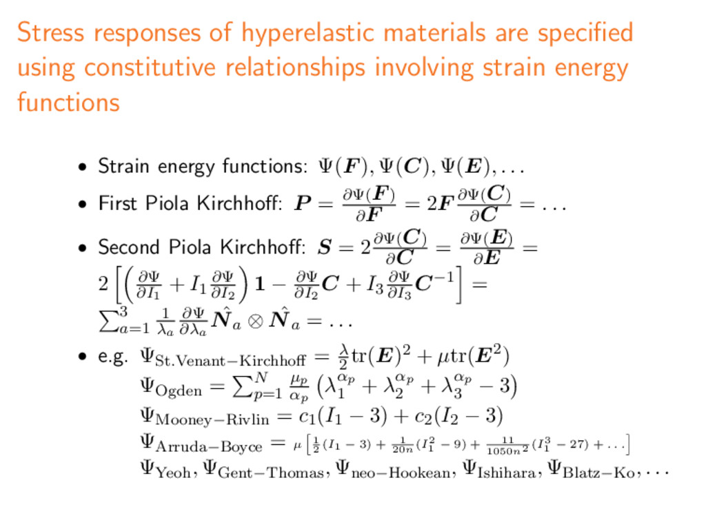
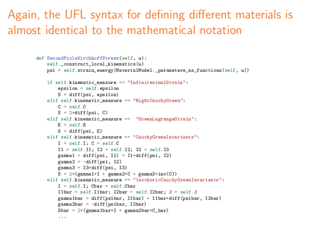
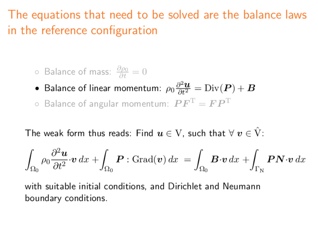
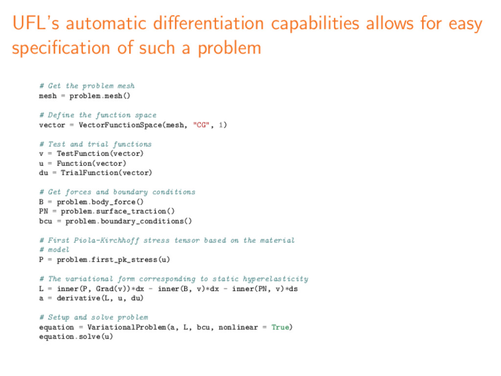
After a brief summary of some key results from classical continuum mechanics, the discourse will turn to the first non-trivial equation of interest: the balance of momentum of a body posed in the reference configuration. We will proceed to show how this classical equation (which is not yet closed, since it does not distinguish one material from another) can be posed generally in weak form using an elegant syntax (in Python) that closely resembles how it is written down on paper. Then, leveraging the automatic linearisation capabilities of the underlying software framework, we will see how one can easily pose sophisticated material models purely at the level of specifying a strain energy function, also using high-level Python syntax. The underlying framework performs the linearisation and generates efficient (C++) code for the finite element computation. Subsequently, information about the computational domain, (Dirichlet and Neumann) boundary conditions, and time-stepping details are each introduced using a few lines of high-level code, completing the specification of the initial- boundary-value problem for nonlinear elasticity. The talk will close with increasingly complex applications of the computational framework.

Transcript

1. An automated computational framework for hyperelasticity Harish Narayanan Center for Biomedical Computing Simula Research Laboratory May 20th, 2010
2. This talk will examine the motivation, design and use of our general framework for hyperelasticity X x B b ϕ Ω0 Ωt P N σn A review of relevant topics from continuum mechanics A brief look at numerical and computational aspects Examples demonstrating the use of the framework
3. Recall, from elementary continuum mechanics . . . X x B b ϕ Ω0 Ωt P N σn The body idealised as a continuous medium Reference and current configurations, body forces and tractions
4. . . . that the motion of solid bodies can be described using different strain measures • Infinitesimal strain: = 1 2 Grad(u) + Grad(u)T • Deformation gradient: F = 1 + Grad(u) • Right Cauchy-Green: C = F TF • Green-Lagrange: E = 1 2 (C − 1) • Left Cauchy-Green: b = F F T • Euler-Almansi: e = 1 2 1 − b−1 • Volumetric and isochoric splits: e.g. J = Det(F ), ¯ C = J− 2 3 C • Invariants of the tensors: I1, I2, I3 • Principal stretches and directions: λ1, λ2, λ3; ˆ N1, ˆ N2, ˆ N3
5. And the UFL syntax for defining these measures is almost identical to the mathematical notation # Infinitesimal strain tensor def InfinitesimalStrain(u): return variable(0.5*(Grad(u) + Grad(u).T)) # Second order identity tensor def SecondOrderIdentity(u): return variable(Identity(u.cell().d)) # Deformation gradient def DeformationGradient(u): I = SecondOrderIdentity(u) return variable(I + Grad(u)) # Determinant of the deformation gradient def Jacobian(u): F = DeformationGradient(u) return variable(det(F)) # Right Cauchy-Green tensor def RightCauchyGreen(u): F = DeformationGradient(u) return variable(F.T*F) # Green-Lagrange strain tensor def GreenLagrangeStrain(u): I = SecondOrderIdentity(u) C = RightCauchyGreen(u) return variable(0.5*(C - I)) # Left Cauchy-Green tensor def LeftCauchyGreen(u): F = DeformationGradient(u) return variable(F*F.T) # Euler-Almansi strain tensor def EulerAlmansiStrain(u): I = SecondOrderIdentity(u) b = LeftCauchyGreen(u) return variable(0.5*(I - inv(b))) # Invariants of an arbitrary tensor, A def Invariants(A): I1 = tr(A) I2 = 0.5*(tr(A)**2 - tr(A*A)) I3 = det(A) return [I1, I2, I3] # Invariants of the (right/left) Cauchy-Green tensor def CauchyGreenInvariants(u): C = RightCauchyGreen(u) [I1, I2, I3] = Invariants(C) return [variable(I1), variable(I2), variable(I3)] # Isochoric part of the deformation gradient def IsochoricDeformationGradient(u): F = DeformationGradient(u) J = Jacobian(u) return variable(J**(-1.0/3.0)*F)
6. Stress responses of hyperelastic materials are specified using constitutive relationships involving strain energy functions • Strain energy functions: Ψ(F ), Ψ(C), Ψ(E), . . . • First Piola Kirchhoff: P = ∂Ψ(F ) ∂F = 2F ∂Ψ(C) ∂C = . . . • Second Piola Kirchhoff: S = 2∂Ψ(C) ∂C = ∂Ψ(E) ∂E = 2 ∂Ψ ∂I1 + I1 ∂Ψ ∂I2 1 − ∂Ψ ∂I2 C + I3 ∂Ψ ∂I3 C−1 = 3 a=1 1 λa ∂Ψ ∂λa ˆ Na ⊗ ˆ Na = . . . • e.g. ΨSt.Venant−Kirchhoff = λ 2 tr(E)2 + μtr(E2) ΨOgden = N p=1 μp αp λαp 1 + λαp 2 + λαp 3 − 3 ΨMooney−Rivlin = c1(I1 − 3) + c2(I2 − 3) ΨArruda−Boyce = µ 1 2 (I1 − 3) + 1 20n (I2 1 − 9) + 11 1050n2 (I3 1 − 27) + . . . ΨYeoh , ΨGent−Thomas , Ψneo−Hookean , ΨIshihara , ΨBlatz−Ko , . . .
7. Again, the UFL syntax for defining different materials is almost identical to the mathematical notation class StVenantKirchhoff(MaterialModel): """Defines the strain energy function for a St. Venant-Kirchhoff material""" def model_info(self): self.num_parameters = 2 self.kinematic_measure = "GreenLagrangeStrain" def strain_energy(self, parameters): E = self.E [mu, lmbda] = parameters return lmbda/2*(tr(E)**2) + mu*tr(E*E) class MooneyRivlin(MaterialModel): """Defines the strain energy function for a (two term) Mooney-Rivlin material""" def model_info(self): self.num_parameters = 2 self.kinematic_measure = "CauchyGreenInvariants" def strain_energy(self, parameters): I1 = self.I1 I2 = self.I2 [C1, C2] = parameters return C1*(I1 - 3) + C2*(I2 - 3)
8. Again, the UFL syntax for defining different materials is almost identical to the mathematical notation def SecondPiolaKirchhoffStress(self, u): self._construct_local_kinematics(u) psi = self.strain_energy(MaterialModel._parameters_as_functions(self, u)) if self.kinematic_measure == "InfinitesimalStrain": epsilon = self.epsilon S = diff(psi, epsilon) elif self.kinematic_measure == "RightCauchyGreen": C = self.C S = 2*diff(psi, C) elif self.kinematic_measure == "GreenLagrangeStrain": E = self.E S = diff(psi, E) elif self.kinematic_measure == "CauchyGreenInvariants": I = self.I; C = self.C I1 = self.I1; I2 = self.I2; I3 = self.I3 gamma1 = diff(psi, I1) + I1*diff(psi, I2) gamma2 = -diff(psi, I2) gamma3 = I3*diff(psi, I3) S = 2*(gamma1*I + gamma2*C + gamma3*inv(C)) elif self.kinematic_measure == "IsochoricCauchyGreenInvariants": I = self.I; Cbar = self.Cbar I1bar = self.I1bar; I2bar = self.I2bar; J = self.J gamma1bar = diff(psibar, I1bar) + I1bar*diff(psibar, I2bar) gamma2bar = -diff(psibar, I2bar) Sbar = 2*(gamma1bar*I + gamma2bar*C_bar) ...
9. The equations that need to be solved are the balance laws in the reference configuration ◦ Balance of mass: ∂ρ0 ∂t = 0 • Balance of linear momentum: ρ0 ∂2u ∂t2 = Div(P ) + B ◦ Balance of angular momentum: P F T = F P T The weak form thus reads: Find u ∈ V, such that ∀ v ∈ ˆ V: Ω0 ρ0 ∂2u ∂t2 ·v dx + Ω0 P : Grad(v) dx = Ω0 B·v dx + ΓN P N·v dx with suitable initial conditions, and Dirichlet and Neumann boundary conditions.
10. UFL’s automatic differentiation capabilities allows for easy specification of such a problem # Get the problem mesh mesh = problem.mesh() # Define the function space vector = VectorFunctionSpace(mesh, "CG", 1) # Test and trial functions v = TestFunction(vector) u = Function(vector) du = TrialFunction(vector) # Get forces and boundary conditions B = problem.body_force() PN = problem.surface_traction() bcu = problem.boundary_conditions() # First Piola-Kirchhoff stress tensor based on the material # model P = problem.first_pk_stress(u) # The variational form corresponding to static hyperelasticity L = inner(P, Grad(v))*dx - inner(B, v)*dx - inner(PN, v)*ds a = derivative(L, u, du) # Setup and solve problem equation = VariationalProblem(a, L, bcu, nonlinear = True) equation.solve(u)
11. UFL’s automatic differentiation capabilities allows for easy specification of such a problem • Spatial derivatives: df i = Dx(f, i) • With respect to user-defined variables: g = variable(cos(cell.x[0])) f = exp(g**2) h = diff(f, g) • Forms with respect to coefficients of a discrete function: a = derivative(L, w, u) • Computing expressions and automatic differentiation: for i = 1, . . . , m : yi = ti = terminal expression dyi dv = dti dv = terminal differentiation rule for i = m + 1, . . . , n : yi = fi (<yj >j∈Ji ) dyi dv = k∈Ji ∂fi ∂yk dyk dv z = yn dz dv = dyn dv
12. A simple static calculation involving a twisted block class Twist(StaticHyperelasticity): def mesh(self): n = 8 return UnitCube(n, n, n) def dirichlet_conditions(self): clamp = Expression(("0.0", "0.0", "0.0")) twist = Expression(("0.0", "y0 + (x[1] - y0) * cos(theta) - (x[2] - z0) * sin(theta) - x[1]", "z0 + (x[1] - y0) * sin(theta) + (x[2] - z0) * cos(theta) - x[2]")) twist.y0 = 0.5 twist.z0 = 0.5 twist.theta = pi/3 return [clamp, twist] def dirichlet_boundaries(self): return ["x[0] == 0.0", "x[0] == 1.0"] def material_model(self): # Material parameters can either be numbers or spatially # varying fields. For example, mu = 3.8461 lmbda = Expression("x[0]*5.8 + (1 - x[0])*5.7") C10 = 0.171; C01 = 4.89e-3; C20 = -2.4e-4; C30 = 5.e-4 #material = MooneyRivlin([mu/2, mu/2]) material = StVenantKirchhoff([mu, lmbda]) #material = Isihara([C10, C01, C20]) #material = Biderman([C10, C01, C20, C30]) return material # Setup and solve the problem twist = Twist() u = twist.solve()
13. A simple static calculation involving a twisted block A solid block twisted by 60 degrees Iteration Res. Norm 1 2.397e+00 2 6.306e-01 3 1.495e-01 4 4.122e-02 5 4.587e-03 6 8.198e-05 7 4.081e-08 8 1.579e-14 Newton scheme convergence
14. The dynamic release of the twisted block class Release(Hyperelasticity): ... def end_time(self): return 10.0 def time_step(self): return 2.e-3 def reference_density(self): return 1.0 def initial_conditions(self): """Return initial conditions for displacement field, u0, and velocity field, v0""" u0 = "twisty.txt" v0 = Expression(("0.0", "0.0", "0.0")) return u0, v0 def dirichlet_conditions(self): clamp = Expression(("0.0", "0.0", "0.0")) return [clamp] def dirichlet_boundaries(self): return ["x[0] == 0.0"] def material_model(self): material = StVenantKirchhoff([3.8461, 5.76]) return material # Setup and solve the problem release = Release() u = release.solve()
15. The dynamic release of the twisted block The relaxation of the released block Conservation of energy
16. A silly hyperelastic fish being forced by a “flow” class FishyFlow(Hyperelasticity): def mesh(self): mesh = Mesh("dolphin.xml.gz") return mesh def end_time(self): return 10.0 def time_step(self): return 0.1 def neumann_conditions(self): flow_push = Expression(("force", "0.0")) flow_push.force = 0.05 return [flow_push] def neumann_boundaries(self): everywhere = "on_boundary" return [everywhere] def material_model(self): material = MooneyRivlin([6.169, 10.15]) return material # Setup and solve the problem fishy = FishyFlow() u = fishy.solve()
17. A silly hyperelastic fish being forced by a “flow” The tumbling of the hyperelastic fish!
18. Concluding remarks, and where you can obtain the code • We have a general framework for isotropic, dynamic hyperelasticity • The following extensions are being worked on: • Implementing other specific material models • Allow for multiple materials and anisotropy • Goal-oriented adaptivity • Introducing coupling with other physics (including FSI) • FEniCS Project: http://fenics.org/ • FEniCS Project Installer: https://launchpad.net/dorsal/ bzr get lp:dorsal • cbc.solve: https://launchpad.net/cbc.solve/ bzr get lp:cbc.solve