A continuum model for the active mechanical response of the myocardium

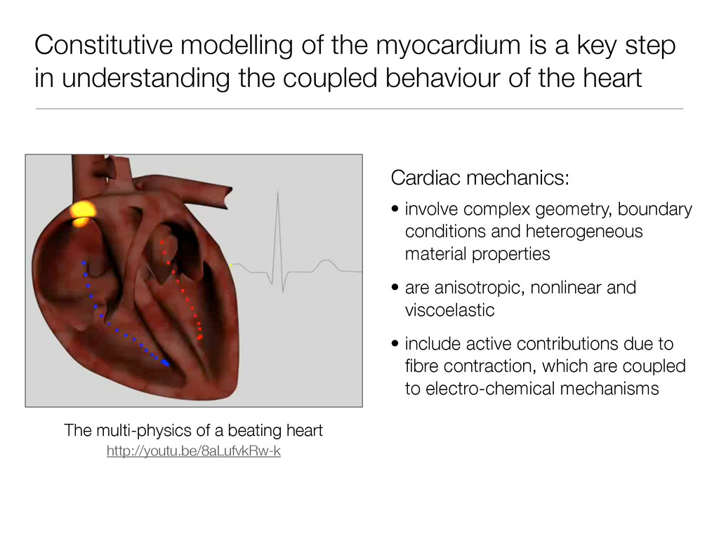
Ventricular myocardium serves as the functional tissue of the heart wall. Driven by intracellular calcium waves, the tissue rhythmically contracts to finite strains. Modelling this behaviour is a key step toward modelling the complex, coupled electro-chemo-mechanical behaviour of the heart.

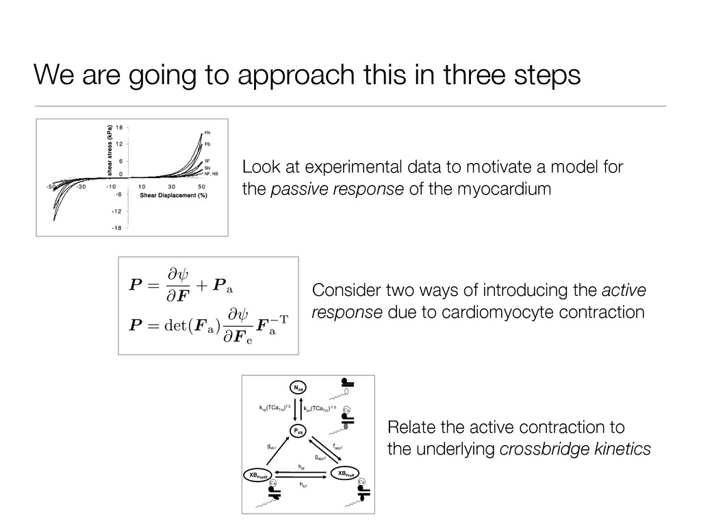
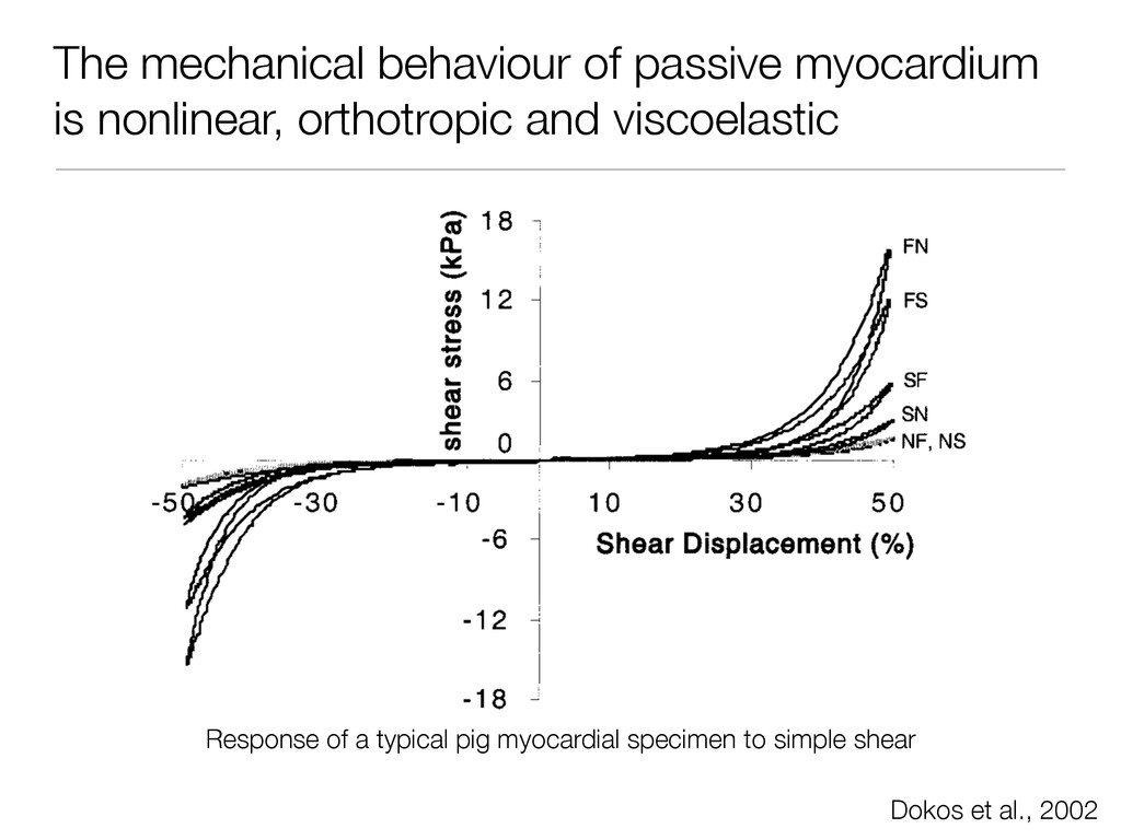
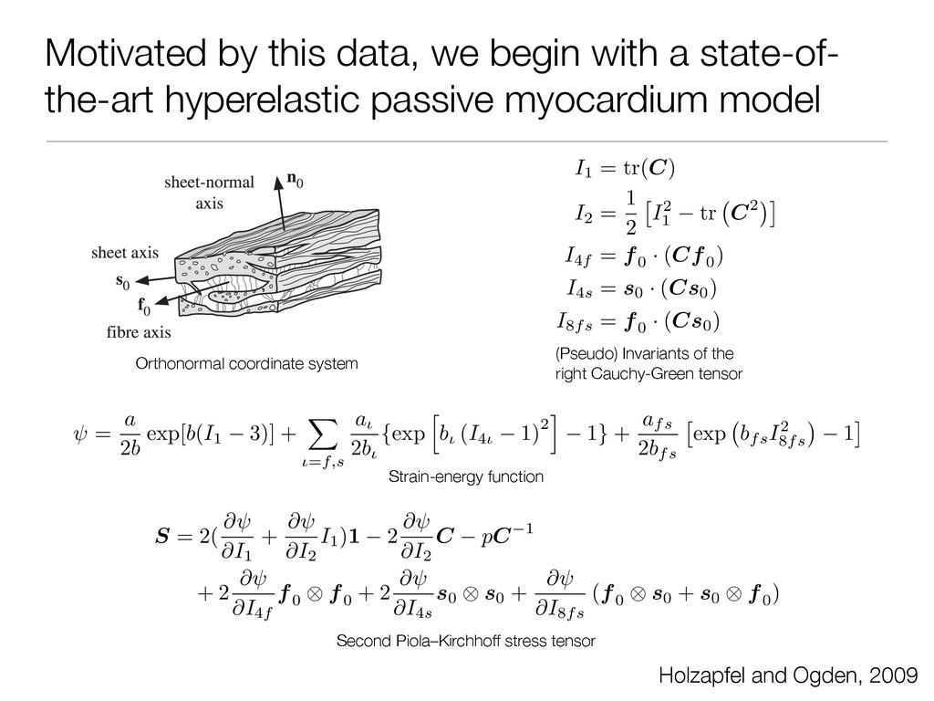
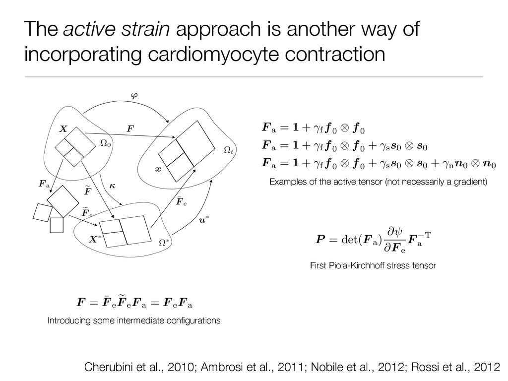
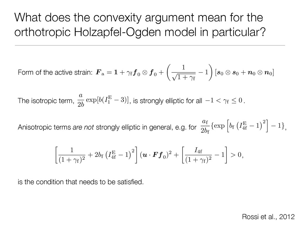
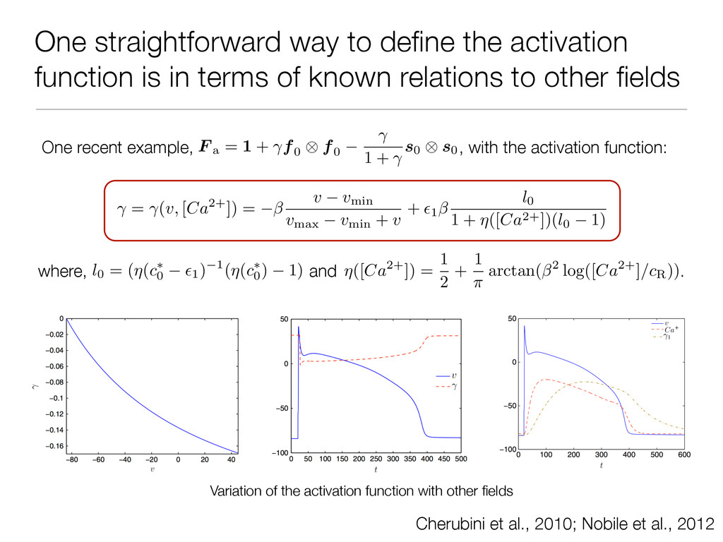
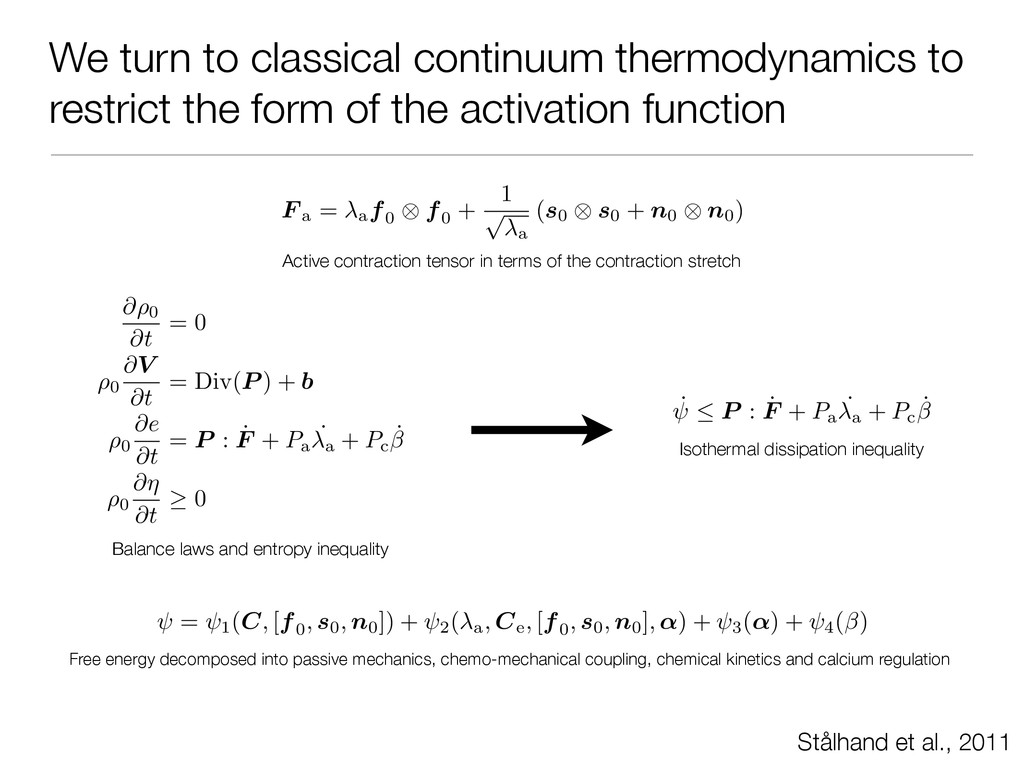
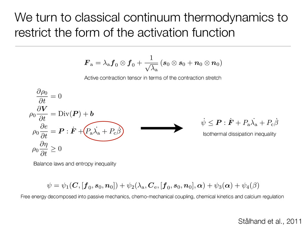
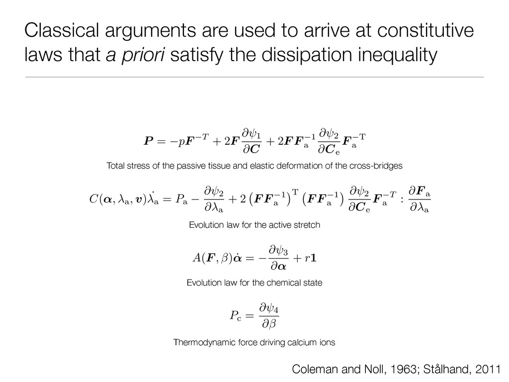
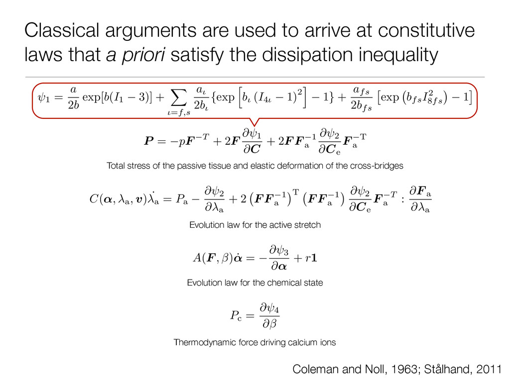
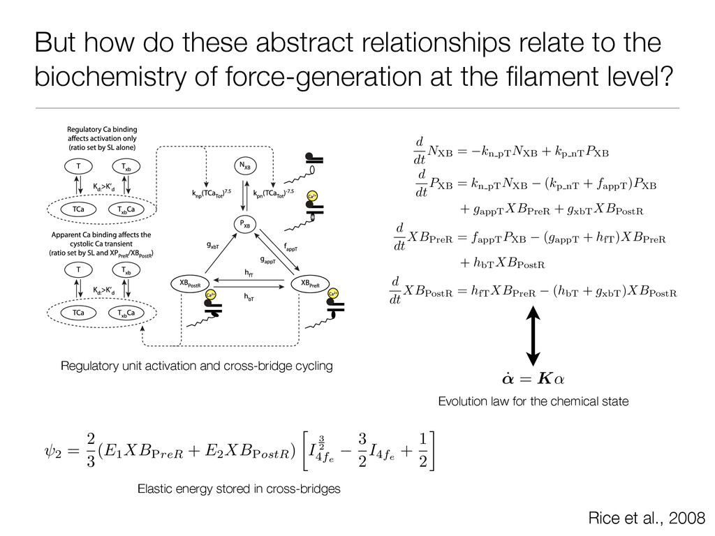
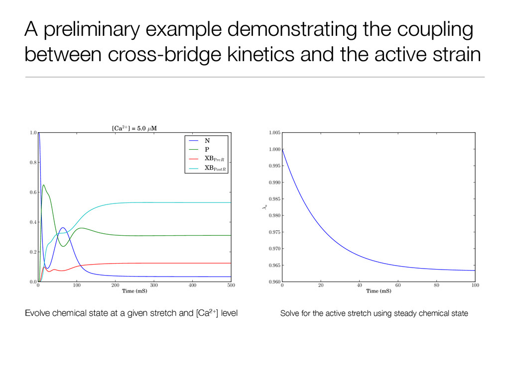
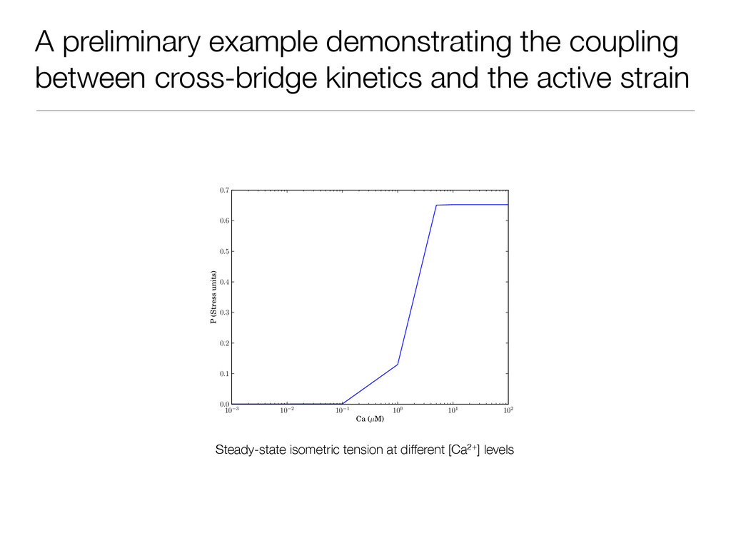
In this exposition, we present a chemo-mechanical formulation posed within the general framework of continuum thermodynamics for describing and studying the active response of the myocardium. Following the recent work of Holzapfel and Ogden (2009), we treat the passive mechanical response of the tissue as non-homogeneous, orthotropic, nonlinear elastic and nearly-incompressible. We then introduce, via a multiplicative decomposition of the deformation gradient (Ambrosi and Pezzuto, 2011), an "active strain" to model the active response of the myocardium. We carefully consider physiological facts to arrive at a suitable functional form for this active strain in terms of active contraction of cardiac muscle fibres. The active fibre contraction is related to the chemical kinetics of crossbridge cycling in cardiac muscles, which we model by a set of ordinary differential equations (Rice et al., 2008).

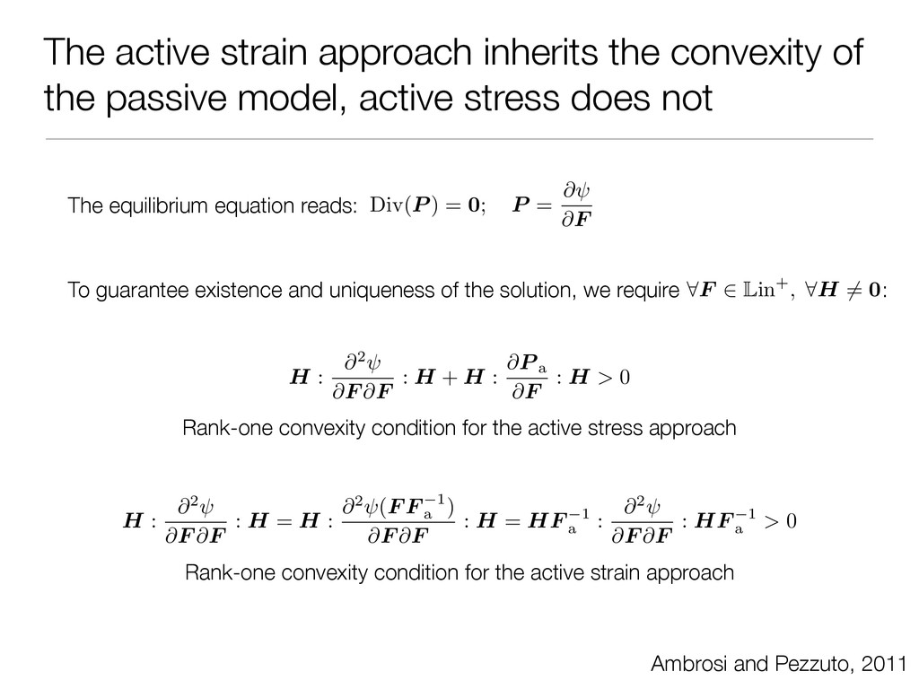
In particular, we will show that the model satisfies key physical properties, including obeying the second law of thermodynamics and ellipticity of the total stress. We conclude with some preliminary numerical results from a finite element numerical implementation of the model, demonstrating aspects of the coupled active response of the myocardium.

Transcript

1. A continuum model for the active mechanical response of the myocardium Harish Narayanan Joakim Sundnes Simula Research Laboratory, Norway Tenth World Congress on Computational Mechanics July 12th, 2012 – São Paulo, Brazil
2. Constitutive modelling of the myocardium is a key step in understanding the coupled behaviour of the heart • involve complex geometry, boundary conditions and heterogeneous material properties • are anisotropic, nonlinear and viscoelastic • include active contributions due to fibre contraction, which are coupled to electro-chemical mechanisms Cardiac mechanics: The multi-physics of a beating heart http://youtu.be/8aLufvkRw-k
3. We are going to approach this in three steps Look at experimental data to motivate a model for the passive response of the myocardium Consider two ways of introducing the active response due to cardiomyocyte contraction Relate the active contraction to the underlying crossbridge kinetics P = @ @F + P a P = det(F a) @ @F e F T a
4. The mechanical behaviour of passive myocardium is nonlinear, orthotropic and viscoelastic Dokos et al., 2002 Response of a typical pig myocardial specimen to simple shear
5. Motivated by this data, we begin with a state-of- the-art hyperelastic passive myocardium model Holzapfel and Ogden, 2009 (Pseudo) Invariants of the right Cauchy-Green tensor Orthonormal coordinate system Strain-energy function Second Piola–Kirchhoff stress tensor I1 = tr(C) I2 = 1 2 ⇥ I2 1 tr C2 ⇤ I4f = f0 · (Cf0 ) I4s = s0 · (Cs0) I8fs = f0 · (Cs0) = a 2 b exp[ b ( I1 3)] + X ◆=f,s a◆ 2 b◆ { exp h b◆ ( I4◆ 1) 2 i 1 } + afs 2 bfs ⇥ exp bfsI2 8fs 1 ⇤ S = 2( @ @I1 + @ @I2 I1)1 2 @ @I2 C pC 1 + 2 @ @I4f f0 ⌦ f0 + 2 @ @I4s s0 ⌦ s0 + @ @I8fs (f0 ⌦ s0 + s0 ⌦ f0 )
6. The Holzapfel-Ogden model fits the loading curve of the experiments closely using eight parameters Holzapfel and Ogden, 2009 Holzapfel-Ogden model fit to experimental data
7. To capture the unload curve as well, we extend this model to include viscous effects Simo, 1987 Volumetric-isochoric decomposition Decoupled representation of the free-energy function Elastic and viscoelastic contributions to the stress Evolution equation for the internal stress variables Specific forms for the strain energy functions C = J 2 3 C, I◆ = Invariants(C) = 1 vol (J) + 1 iso (C) + m X ↵ =1 ↵(C, ↵) S = S1 vol + S1 iso + m X ↵ =1 Q↵ S1 vol = J @ 1 vol (J) @J C 1 S1 iso = J 2 3 Dev ✓ 2 @ 1 iso (C) @C ◆ ˙ Q↵ + Q↵ ⌧↵ = ↵ ˙ S1 iso (C), Q↵ |t =0 = 0 1 iso = a 2 b exp[ b ( I 1 3)] + X ◆ = f,s a◆ 2 b◆ { exp h b◆ I 4 ◆ 1 2 i 1 } + afs 2 bfs h exp ⇣ bfsI2 8 fs ⌘ 1 i 1 vol =   1 2 ✓ ln J + 1 J 1 ◆
8. 0.5 0.3 0.1 0.0 0.1 0.3 0.5 Shear strain 18 12 6 0 6 12 18 Shear stress (kPa) sf nf fs ns fn sn With two additional parameters related to viscoelasticity, our model further captures the data Experimental data from Dokos et al., 2002 ⌧1 1 Our viscoelastic model with = 1.5 s, = 0.25
9. The active stress approach is an intuitive way of incorporating cardiomyocyte contraction Examples of the active stress tensor Additional active contribution to the stress Smith et al., 2004; Panfilov et al., 2005; Niederer and Smith, 2008; Pathmanathan et al., 2010 P a = Ta F C 1 P a = Ta F f0 ⌦ f0 P a = Taff F f0 ⌦ f0 + Tass F s0 ⌦ s0 + Tann F n0 ⌦ n0 P = P p + P a = @ @F + P a
10. The active strain approach is another way of incorporating cardiomyocyte contraction Introducing some intermediate configurations First Piola-Kirchhoff stress tensor Examples of the active tensor (not necessarily a gradient) Cherubini et al., 2010; Ambrosi et al., 2011; Nobile et al., 2012; Rossi et al., 2012 F = ¯ F e e F eF a = F eF a P = det(F a) @ @F e F T a F a = 1 + f f0 ⌦ f0 F a = 1 + f f0 ⌦ f0 + ss0 ⌦ s0 F a = 1 + f f0 ⌦ f0 + ss0 ⌦ s0 + nn0 ⌦ n0 Ω0 Ω∗ Ωt X X∗ x F a F e F ¯ F e F κ u∗ ϕ
11. The active strain approach inherits the convexity of the passive model, active stress does not Rank-one convexity condition for the active strain approach Rank-one convexity condition for the active stress approach Ambrosi and Pezzuto, 2011 The equilibrium equation reads: To guarantee existence and uniqueness of the solution, we require : Div(P ) = 0; P = @ @F 8F 2 Lin+, 8H 6= 0 H : @2 @F @F : H + H : @P a @F : H > 0 H : @2 @F @F : H = H : @2 (F F 1 a ) @F @F : H = HF 1 a : @2 @F @F : HF 1 a > 0
12. The active strain approach inherits the convexity of the passive model, active stress does not Rank-one convexity condition for the active strain approach Rank-one convexity condition for the active stress approach Ambrosi and Pezzuto, 2011 The equilibrium equation reads: To guarantee existence and uniqueness of the solution, we require : Div(P ) = 0; P = @ @F 8F 2 Lin+, 8H 6= 0 H : @2 @F @F : H + H : @P a @F : H > 0 H : @2 @F @F : H = H : @2 (F F 1 a ) @F @F : H = HF 1 a : @2 @F @F : HF 1 a > 0
13. What does the convexity argument mean for the orthotropic Holzapfel-Ogden model in particular? Rossi et al., 2012 is the condition that needs to be satisfied. Form of the active strain: F a = 1 + f f0 ⌦ f0 + ✓ 1 p 1 + f 1 ◆ [s0 ⌦ s0 + n0 ⌦ n0] The isotropic term, , is strongly elliptic for all . 1 < f  0 a 2 b exp[ b ( IE 1 3)] ,  1 (1 + f )2 + 2bf IE 4f 1 2 (u · F f0 )2 +  I4f (1 + f )2 1 > 0 Anisotropic terms are not strongly elliptic in general, e.g. for , af 2 bf { exp h bf IE 4f 1 2 i 1 }
14. A numerical example where the active strain formulation easily allows for large strains Form of the active strain: F a = 1 + f f0 ⌦ f0 + ✓ 1 p 1 + f 1 ◆ [s0 ⌦ s0 + n0 ⌦ n0] Toy activation function within the physiological range: f (t) = 0.15 [1 sin(t 3⇡/2)]
15. One straightforward way to define the activation function is in terms of known relations to other fields Cherubini et al., 2010; Nobile et al., 2012 Variation of the activation function with other fields One recent example, , with the activation function: F a = 1 + f0 ⌦ f0 1 + s0 ⌦ s0 = (v, [Ca2+]) = v v min v max v min + v + ✏ 1 l 0 1 + ⌘([Ca2+ ])(l 0 1) where, and . l0 = (⌘(c⇤ 0 ✏1) 1(⌘(c⇤ 0 ) 1) ⌘ ([ Ca2+ ]) = 1 2 + 1 ⇡ arctan( 2 log([ Ca2+ ] /cR))
16. We turn to classical continuum thermodynamics to restrict the form of the activation function Stålhand et al., 2011 Active contraction tensor in terms of the contraction stretch F a = af0 ⌦ f0 + 1 p a (s0 ⌦ s0 + n0 ⌦ n0) Balance laws and entropy inequality @⇢0 @t = 0 ⇢0 @V @t = Div(P ) + b ⇢0 @e @t = P : ˙ F + Pa ˙ a + Pc ˙ ⇢0 @⌘ @t 0 Isothermal dissipation inequality ˙  P : ˙ F + Pa ˙ a + Pc ˙ Free energy decomposed into passive mechanics, chemo-mechanical coupling, chemical kinetics and calcium regulation = 1(C, [f0 , s0, n0]) + 2( a, Ce, [f0 , s0, n0], ↵) + 3(↵) + 4( )
17. We turn to classical continuum thermodynamics to restrict the form of the activation function Stålhand et al., 2011 Active contraction tensor in terms of the contraction stretch F a = af0 ⌦ f0 + 1 p a (s0 ⌦ s0 + n0 ⌦ n0) Balance laws and entropy inequality @⇢0 @t = 0 ⇢0 @V @t = Div(P ) + b ⇢0 @e @t = P : ˙ F + Pa ˙ a + Pc ˙ ⇢0 @⌘ @t 0 Isothermal dissipation inequality ˙  P : ˙ F + Pa ˙ a + Pc ˙ Free energy decomposed into passive mechanics, chemo-mechanical coupling, chemical kinetics and calcium regulation = 1(C, [f0 , s0, n0]) + 2( a, Ce, [f0 , s0, n0], ↵) + 3(↵) + 4( )
18. Classical arguments are used to arrive at constitutive laws that a priori satisfy the dissipation inequality Coleman and Noll, 1963; Stålhand, 2011 Total stress of the passive tissue and elastic deformation of the cross-bridges P = pF T + 2F @ 1 @C + 2F F 1 a @ 2 @Ce F T a Evolution law for the active stretch C(↵, a, v) ˙ a = Pa @ 2 @ a + 2 F F 1 a T F F 1 a @ 2 @Ce F T a : @F a @ a Evolution law for the chemical state A(F , ) ˙ ↵ = @ 3 @↵ + r1 Thermodynamic force driving calcium ions Pc = @ 4 @
19. Classical arguments are used to arrive at constitutive laws that a priori satisfy the dissipation inequality Coleman and Noll, 1963; Stålhand, 2011 Total stress of the passive tissue and elastic deformation of the cross-bridges P = pF T + 2F @ 1 @C + 2F F 1 a @ 2 @Ce F T a 1 = a 2 b exp[ b ( I1 3)] + X ◆=f,s a◆ 2 b◆ { exp h b◆ ( I4◆ 1) 2 i 1 } + afs 2 bfs ⇥ exp bfsI2 8fs 1 ⇤ Evolution law for the active stretch C(↵, a, v) ˙ a = Pa @ 2 @ a + 2 F F 1 a T F F 1 a @ 2 @Ce F T a : @F a @ a Evolution law for the chemical state A(F , ) ˙ ↵ = @ 3 @↵ + r1 Thermodynamic force driving calcium ions Pc = @ 4 @
20. But how do these abstract relationships relate to the biochemistry of force-generation at the filament level? Regulatory unit activation and cross-bridge cycling Rice et al., 2008 Evolution law for the chemical state Elastic energy stored in cross-bridges d dt N XB = k n pT N XB + k p nT P XB d dt P XB = k n pT N XB (k p nT + f appT )P XB + g appT XB PreR + g xbT XB PostR d dt XB PreR = f appT P XB (g appT + h fT )XB PreR + h bT XB PostR d dt XB PostR = h fT XB PreR (h bT + g xbT )XB PostR ˙ ↵ = K↵ 2 = 2 3 (E1XBP reR + E2XBP ostR )  I 3 2 4 fe 3 2 I4 fe + 1 2
21. A preliminary example demonstrating the coupling between cross-bridge kinetics and the active strain 0 100 200 300 400 500 Time (mS) 0.0 0.2 0.4 0.6 0.8 1.0 [Ca2+] = 5.0 µM N P XBPreR XBPostR Evolve chemical state at a given stretch and [Ca2+] level 0 20 40 60 80 100 Time (mS) 0.960 0.965 0.970 0.975 0.980 0.985 0.990 0.995 1.000 1.005 a Solve for the active stretch using steady chemical state
22. A preliminary example demonstrating the coupling between cross-bridge kinetics and the active strain 10 3 10 2 10 1 100 101 102 Ca (µM) 0.0 0.1 0.2 0.3 0.4 0.5 0.6 0.7 P (Stress units) Steady-state isometric tension at different [Ca2+] levels
23. Summarising remarks, and some points for discussion • We are building a chemo-mechanical continuum model for characterising and studying the behaviour of the cardiac myocardium • We use a viscoelastic passive model based on a modern hyperelastic law • We explored some arguments to choose the active strain approach • We use continuum thermodynamics and biophysics to motivate the form of the active strain
24. Summarising remarks, and some points for discussion • We are building a chemo-mechanical continuum model for characterising and studying the behaviour of the cardiac myocardium • We use a viscoelastic passive model based on a modern hyperelastic law • We explored some arguments to choose the active strain approach • We use continuum thermodynamics and biophysics to motivate the form of the active strain • More work is needed in tying the abstract formulation to underlying biophysics • The importance of viscosity is not clear, but I am exploring its role in energy dissipation and starting to look at whether this helps with numerical stability • Much of the results you saw today were generated using open source Python code, so ask me for it if you’d like to play too! http://harishnarayanan.org/