Item Response Theory

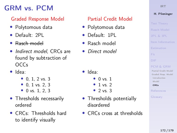
These are the slides for the seminar "New Developments in Testtheory and Test Construction" (University of Mannheim, Master Psychology). Therein, models within the framework of item response theory (IRT) are presented, discussed, and illustrated with examples. More specifically, models for binary data such as the Rasch, the 2PL, and the 3PL model are discussed as well as models for ordinal data such as the partial credit model (PCM) and the graded response model (GRM). Furthermore, specific chapters are dedicated to item/test information, parameter estimation, item/model fit, and differential item functioning (DIF).

Transcript

1. IRT H. Plieninger Test Theory Rasch Model 2PL & 3PL Item Information Estimation Fit DIF PCM & GRM References Glossary Item Response Theory Hansjörg Plieninger University of Mannheim 1 / 179
2. IRT H. Plieninger Test Theory Rasch Model 2PL & 3PL Item Information Estimation Fit DIF PCM & GRM References Glossary License • This is version 1.0.0 of this slidedeck. • Please report any errata. mail@hansjoerg.me hansjoerg_me https://www.hansjoerg.me • This work is licensed under a Creative Commons Attribution 4.0 International License. 2 / 179
3. IRT H. Plieninger Test Theory Rasch Model 2PL & 3PL Item Information Estimation Fit DIF PCM & GRM References Glossary Table of Contents 1 Test Theory 2 Rasch Model 3 2PL and 3PL Model 4 Item and Test Information 5 Parameter Estimation 6 Item and Model Fit 7 Differential Item Functioning 8 Polytomous IRT Models 3 / 179
4. IRT H. Plieninger Test Theory Rasch Model 2PL & 3PL Item Information Estimation Fit DIF PCM & GRM References Glossary TOC: Test Theory 1 Test Theory 4 / 179
5. IRT H. Plieninger Test Theory Rasch Model 2PL & 3PL Item Information Estimation Fit DIF PCM & GRM References Glossary What is a Test? • A scientific procedure used to assess an individual’s standing on a certain attribute • Personally, I often call all psychometric procedures tests, but some people differentiate between tests and questionnaires etc. 5 / 179
6. IRT H. Plieninger Test Theory Rasch Model 2PL & 3PL Item Information Estimation Fit DIF PCM & GRM References Glossary What is (a) Test Theory? Testtheorien ngen der Testtheorie und Testkonstruktion 5 Abbildung modifiziert nach Rost (2004), S. 21 Attribute Response indicative of influences Scoring Test theory le Steinwascher (Rost, 2004, p. 20) • Test theory: How does an attribute influence test responses • If the response is sufficient, no need for a theory (e.g., party vote) • You may take the response (e.g., sum score) at face value, but • You make implicit assumptions • You have to show post hoc that it’s meaningful 6 / 179
7. IRT H. Plieninger Test Theory Rasch Model 2PL & 3PL Item Information Estimation Fit DIF PCM & GRM References Glossary What is (a) Test Theory? • A theory aims at describing and explaining behavior (X) as a function of persons and situations: X = f (P, S) • Empirically observed behavior: S1 S2 S3 P1 1 1 0 P2 1 0 0 • Goal 1: Infer attribute from behavior (e.g., P1 is very intelligent) • Goal 2: Compare persons (e.g., P1 is more intelligent than P2 ) • For this, a formal model is needed: Prob(X) = f (PropertyPerson , PropertySituation ) 7 / 179
8. IRT H. Plieninger Test Theory Rasch Model 2PL & 3PL Item Information Estimation Fit DIF PCM & GRM References Glossary What is a Formal Model? • A reduced description of natural phenomena • “All models are wrong but some are useful” (George Box) • The phenomena are described using parameters • Those are estimated from observed data • A model may exist as a mathematical expression alone, but filled with content it becomes a theory 8 / 179
9. IRT H. Plieninger Test Theory Rasch Model 2PL & 3PL Item Information Estimation Fit DIF PCM & GRM References Glossary Test Theory and Formal Models? • A test theory (e.g., IRT) is rather not a single and concrete theory (e.g., like dual process theory) • It’s rather an abstract framework for a set of formal models • For example, in IRT, we have • Formal models for binary responses (e.g, Rasch, 2PL) • Formal models for polytomous responses (e.g., PCM) • . . . • Test construction: • Top-down: Model in mind, develop material accordingly • Bottom-up: Problem at hand, select/develop model accordingly 9 / 179
10. IRT H. Plieninger Test Theory Rasch Model 2PL & 3PL Item Information Estimation Fit DIF PCM & GRM References Glossary Description and Explanation • A theory aims at both describing and explaining natural phenomena • Up to now, this sounds all very descriptive • Explanatory part: Observed responses are explained by means of latent variables • Byproduct: Observed – ordinal; latent – interval 10 / 179
11. IRT H. Plieninger Test Theory Rasch Model Introduction Model LLTM Example Paper 2PL & 3PL Item Information Estimation Fit DIF PCM & GRM References Glossary TOC: Rasch Model 2 Rasch Model Introduction Model LLTM Example Paper 11 / 179
12. IRT H. Plieninger Test Theory Rasch Model Introduction Data Structure Graphical Model Formal Model Model LLTM Example Paper 2PL & 3PL Item Information Estimation Fit DIF PCM & GRM References Glossary Dichotomous Items • Test data are often dichotomous • Often scored with 0s and 1s → binary • Sometimes (in CTT), aggregation across items to get a “continuous” outcome • Here, we want to focus on the dis-aggregated data Example: √ 9 + 16 =? √ 9 + 16 = 5 (1, correct) √ 9 + 16 = 25 (0, wrong) 12 / 179
13. IRT H. Plieninger Test Theory Rasch Model Introduction Data Structure Graphical Model Formal Model Model LLTM Example Paper 2PL & 3PL Item Information Estimation Fit DIF PCM & GRM References Glossary Dichotomous Items • Test data are often dichotomous • Often scored with 0s and 1s → binary • Sometimes (in CTT), aggregation across items to get a “continuous” outcome • Here, we want to focus on the dis-aggregated data Example: “I don’t talk a lot” agree (1) disagree (0) 13 / 179
14. IRT H. Plieninger Test Theory Rasch Model Introduction Data Structure Graphical Model Formal Model Model LLTM Example Paper 2PL & 3PL Item Information Estimation Fit DIF PCM & GRM References Glossary Data Structure • Person j = 1, . . . , J • Item i = 1 . . . , I • Response xji = 0, 1 • Sum score rj = I i=1 xji • Assumption: Sum score is unidimensional and ordinal V1 V2 V3 V4 rj 1 0 1 1 0 2 2 0 0 0 1 1 3 0 1 1 1 3 4 1 1 1 0 3 5 1 0 1 0 2 14 / 179
15. IRT H. Plieninger Test Theory Rasch Model Introduction Data Structure Graphical Model Formal Model Model LLTM Example Paper 2PL & 3PL Item Information Estimation Fit DIF PCM & GRM References Glossary A Binary Item: Linear Model 0 5 10 15 20 25 0 1 Sum Score Response 15 / 179
16. IRT H. Plieninger Test Theory Rasch Model Introduction Data Structure Graphical Model Formal Model Model LLTM Example Paper 2PL & 3PL Item Information Estimation Fit DIF PCM & GRM References Glossary A Binary Item: Guttman 0 5 10 15 20 25 0 1 Sum Score Response 16 / 179
17. IRT H. Plieninger Test Theory Rasch Model Introduction Data Structure Graphical Model Formal Model Model LLTM Example Paper 2PL & 3PL Item Information Estimation Fit DIF PCM & GRM References Glossary A Binary Item: S-Shaped 0 5 10 15 20 25 0.0 0.2 0.4 0.6 0.8 1.0 Sum Score Proportion 17 / 179
18. IRT H. Plieninger Test Theory Rasch Model Introduction Data Structure Graphical Model Formal Model Model LLTM Example Paper 2PL & 3PL Item Information Estimation Fit DIF PCM & GRM References Glossary Seeking a Formal Model (i.e., f ) • Should be parsimonious (Occam’s razor) • Should be statistically convenient (easy to estimate) • Should be psychologically plausible • P(Xji = 1) = fi (θj ) • Range of fi must be [0, 1] • fi is often monotonically increasing • fi is the item characteristic curve (ICC) of item i 18 / 179
19. IRT H. Plieninger Test Theory Rasch Model Introduction Data Structure Graphical Model Formal Model Model LLTM Example Paper 2PL & 3PL Item Information Estimation Fit DIF PCM & GRM References Glossary Notation θ Person parameter (e.g., ability) β Item difficulty parameter xji Observed response of person j to item i (e.g., x5,2 = 1) Xji Random variable that can take on values of 0 and 1 P(Xji = 1) Probability (P) that the random variable Xji takes on the value of 1 log Natural logarithm: log(ex ) = log(exp(x)) = x 19 / 179
20. IRT H. Plieninger Test Theory Rasch Model Introduction Data Structure Graphical Model Formal Model Model LLTM Example Paper 2PL & 3PL Item Information Estimation Fit DIF PCM & GRM References Glossary CTT for Binary Items Linear model: • Xji = θj − βi • Problem: Out of range predictions Binomial model: • P(Xji = 1) = θj − βi • Probabilistic: Good • Problem: Range restriction for θ and β, because (θj − βi ) must not exceed interval of [0, 1] 20 / 179
21. IRT for Binary Items 1 Starting point: Probability P(Xji = 1) Range: [0, 1] 2 Transformation I: Odds P(Xji = 1) P(Xji = 0) Range: [0, ∞) 3 Transformation II: Logarithm → logit log P(Xji = 1) P(Xji = 0) Range: (−∞, ∞) P Odds Logit 0.00 0.00 −∞ 0.10 0.11 −2.20 . . . . . . . . . 0.50 1.00 0.00 0.60 1.50 0.41 0.70 2.33 0.85 0.80 4.00 1.39 0.90 9.00 2.20 1.00 +∞ +∞
22. IRT H. Plieninger Test Theory Rasch Model Introduction Data Structure Graphical Model Formal Model Model LLTM Example Paper 2PL & 3PL Item Information Estimation Fit DIF PCM & GRM References Glossary IRT for Binary Items • Since the logit has range (−∞, ∞), we can use anything (e.g., something linear) for the right-hand side: log P(Xji = 1) P(Xji = 0) = θj − βi • The larger θj (the more able person j), the larger the left-hand side • The larger βi (the more difficult item i), the smaller the left-hand side 22 / 179
23. IRT H. Plieninger Test Theory Rasch Model Introduction Data Structure Graphical Model Formal Model Model LLTM Example Paper 2PL & 3PL Item Information Estimation Fit DIF PCM & GRM References Glossary IRT for Binary Items log P(Xji = 1) P(Xji = 0) = θj − βi log p1 p0 = a |p0 = 1 − p1 log p1 1 − p1 = a | exp p1 1 − p1 = exp(a) | ∗ (1 − p1) p1 = (1 − p1) ∗ exp(a) p1 = exp(a) − p1 ∗ exp(a) | + p1 ∗ exp(a) p1 + p1 ∗ exp(a) = exp(a) p1(1 + exp(a)) = exp(a) | : (1 + exp(a)) p1 = exp(a) 1 + exp(a) 23 / 179
24. IRT H. Plieninger Test Theory Rasch Model Introduction Model ICCs Interpretation Specific Objectivity Local Independence Sufficient Statistics Model Identification LLTM Example Paper 2PL & 3PL Item Information Estimation Fit DIF PCM & GRM References Glossary Rasch Model Rasch model (Rasch, 1960) P(Xji = 1) = exp(θj − βi ) 1 + exp(θj − βi ) Rasch model in logit notation logit(P) = log P(Xji = 1) P(Xji = 0) = ηji = θj − βi • Sometimes, the more precise notation of a conditional probability is used: P(Xji = 1|θj , βi ) • This means that the probability depends/is conditional on θj and βi 24 / 179
25. IRT H. Plieninger Test Theory Rasch Model Introduction Model ICCs Interpretation Specific Objectivity Local Independence Sufficient Statistics Model Identification LLTM Example Paper 2PL & 3PL Item Information Estimation Fit DIF PCM & GRM References Glossary Logistic Function -5 -3 -1 1 3 5 0.0 0.2 0.4 0.6 0.8 1.0 y = ex 1 + ex x y 25 / 179
26. IRT H. Plieninger Test Theory Rasch Model Introduction Model ICCs Interpretation Specific Objectivity Local Independence Sufficient Statistics Model Identification LLTM Example Paper 2PL & 3PL Item Information Estimation Fit DIF PCM & GRM References Glossary ICC for a Single Rasch Item -5 -3 -1 1 3 5 0.0 0.2 0.4 0.6 0.8 1.0 q Prob bi = 0 26 / 179
27. IRT H. Plieninger Test Theory Rasch Model Introduction Model ICCs Interpretation Specific Objectivity Local Independence Sufficient Statistics Model Identification LLTM Example Paper 2PL & 3PL Item Information Estimation Fit DIF PCM & GRM References Glossary ICC for a Single Rasch Item -5 -3 -1 1 3 5 0.0 0.2 0.4 0.6 0.8 1.0 q Prob bi = 0 • y-axis: Probability P(Xji = 1) • x-axis: θ (units: logits) • βi : Inflection point (ICC turns from convex to concave) → item difficulty • βi : P = 50% • Upper (lower) asymptote of 1 (0) • Monotonically increasing: Flat, curved, linear, curved, flat • Discrimination 27 / 179
28. IRT H. Plieninger Test Theory Rasch Model Introduction Model ICCs Interpretation Specific Objectivity Local Independence Sufficient Statistics Model Identification LLTM Example Paper 2PL & 3PL Item Information Estimation Fit DIF PCM & GRM References Glossary ICC for a Single Rasch Item -5 -3 -1 1 3 5 0.0 0.2 0.4 0.6 0.8 1.0 q Prob bi = 0 P(Xji = 0) P(Xji = 1) 28 / 179
29. IRT H. Plieninger Test Theory Rasch Model Introduction Model ICCs Interpretation Specific Objectivity Local Independence Sufficient Statistics Model Identification LLTM Example Paper 2PL & 3PL Item Information Estimation Fit DIF PCM & GRM References Glossary ICCs for Four Rasch Items -5 -3 -1 1 3 5 0.0 0.2 0.4 0.6 0.8 1.0 q Prob 29 / 179
30. IRT H. Plieninger Test Theory Rasch Model Introduction Model ICCs Interpretation Specific Objectivity Local Independence Sufficient Statistics Model Identification LLTM Example Paper 2PL & 3PL Item Information Estimation Fit DIF PCM & GRM References Glossary Interpretation (Greb, 2007; Moosbrugger & Kelava, 2012) 30 / 179
31. IRT H. Plieninger Test Theory Rasch Model Introduction Model ICCs Interpretation Specific Objectivity Local Independence Sufficient Statistics Model Identification LLTM Example Paper 2PL & 3PL Item Information Estimation Fit DIF PCM & GRM References Glossary Advantages of IRT/Rasch Models • IRT is helpful for developing homogeneous, construct valid tests • IRT facilitates the interpretation of the person and item parameters (both are measured on the same scale) • Sample invariance in the Rasch model • “In CTT, the meaning of a score results from comparing its position on a standard, namely a norm group” (Embretson & Reise, 2000, p. 126) • “In IRT, trait levels have meaning in comparison to items” (Embretson & Reise, 2000, p. 127) 31 / 179
32. IRT H. Plieninger Test Theory Rasch Model Introduction Model ICCs Interpretation Specific Objectivity Local Independence Sufficient Statistics Model Identification LLTM Example Paper 2PL & 3PL Item Information Estimation Fit DIF PCM & GRM References Glossary Specific Objectivity • “Rasch (1977) developed the concept of specific objectivity as a general scientific principle; namely, comparisons between objects must be generalizable beyond the specific conditions under which they were observed.” (Embretson & Reise, 2000, p. 143) • Comparisons between persons should not depend on the specific items administered • Comparisons between items should not depend on the persons that were tested 32 / 179
33. IRT H. Plieninger Test Theory Rasch Model Introduction Model ICCs Interpretation Specific Objectivity Local Independence Sufficient Statistics Model Identification LLTM Example Paper 2PL & 3PL Item Information Estimation Fit DIF PCM & GRM References Glossary Specific Objectivity The difference between two Persons θ1 and θ2 is independent of the item at hand: log P(X1i = 1) P(X1i = 0) − log P(X2i = 1) P(X2i = 0) = (θ1 − βi ) − (θ2 − βi ) = θ1 − θ2 The difference between two items β1 and β2 is independent of the person at hand: log P(Xj1 = 1) P(Xj1 = 0) − log P(Xj2 = 1) P(Xj2 = 0) = (θj − β1) − (θj − β2) = −β1 + β2 33 / 179
34. IRT H. Plieninger Test Theory Rasch Model Introduction Model ICCs Interpretation Specific Objectivity Local Independence Sufficient Statistics Model Identification LLTM Example Paper 2PL & 3PL Item Information Estimation Fit DIF PCM & GRM References Glossary Sample Invariance • Specific objectivity leads to the sample invariance property of the Rasch model • Restriction • Holds only within the Rasch model (e.g., not for the 2PL) • Holds for relative (not absolute) differences (→ identification) • Is a property of the population model; the estimates become, of course, more accurate when using “appropriate” items/persons (→ item/test information) • Holds within a homogeneous population (→ DIF) 34 / 179
35. IRT H. Plieninger Test Theory Rasch Model Introduction Model ICCs Interpretation Specific Objectivity Local Independence Sufficient Statistics Model Identification LLTM Example Paper 2PL & 3PL Item Information Estimation Fit DIF PCM & GRM References Glossary Local Independence • Central assumption • At a given θ-level (i.e., locally), the probability of an event must not depend on the outcome of a previous event (i.e., item) • Also assumed for persons • Allows to multiply individual probabilities (disregarding interactions), which is needed for the likelihood-function (→ estimation) • Comparable to uncorrelated errors in CTT or independent dice throws 35 / 179
36. IRT H. Plieninger Test Theory Rasch Model Introduction Model ICCs Interpretation Specific Objectivity Local Independence Sufficient Statistics Model Identification LLTM Example Paper 2PL & 3PL Item Information Estimation Fit DIF PCM & GRM References Glossary Violation of Local Independence Local independence may be violated: • If items build on each other, especially in the case of testlets • If tests aren’t unidimensional (e.g., math test including word problems) • Order or trainings effects within a test • Answer copying • Independence has to be ensured by means of test design/material/administration • Hard to test post hoc • May be directly modeled (e.g., testlets, multidimensionality) 36 / 179
37. IRT H. Plieninger Test Theory Rasch Model Introduction Model ICCs Interpretation Specific Objectivity Local Independence Sufficient Statistics Model Identification LLTM Example Paper 2PL & 3PL Item Information Estimation Fit DIF PCM & GRM References Glossary Sufficient Statistics • A sufficient statistic is a statistic that carries all relevant information about an unknown parameter • In the Rasch model, the sum score (row sum, rj = I i=1 xji ) is a sufficient statistic for θj , → For θj , it’s irrelevant which items were solved, only how many is important • Likewise, the item sum score (column sum, ci = J j=1 xji ) is a sufficient statistic for βi • Sufficient statistics may facilitate parameter estimation, because it can be shown that one can compute the likelihood on the basis of the sum scores (without knowing the actual xji s) 37 / 179
38. IRT H. Plieninger Test Theory Rasch Model Introduction Model ICCs Interpretation Specific Objectivity Local Independence Sufficient Statistics Model Identification LLTM Example Paper 2PL & 3PL Item Information Estimation Fit DIF PCM & GRM References Glossary Consequences of Sufficient Statistics If the Rasch model holds: • The sum score is comparable to the person parameter • Weighting the items is unnecessary and even wrong • Response patterns carry no information beyond the person parameters 38 / 179
39. IRT H. Plieninger Test Theory Rasch Model Introduction Model ICCs Interpretation Specific Objectivity Local Independence Sufficient Statistics Model Identification LLTM Example Paper 2PL & 3PL Item Information Estimation Fit DIF PCM & GRM References Glossary Identification • The scale of a latent variable is always unknown • The parameters in the Rasch model are only identified up to an additive constant: log P(X1i = 1) P(X1i = 0) = θj − βi = (θj + c) − (βj + c) 1 = 3 − 2 = 137 − 136 • The location of the scale has to be fixed by the researcher (in an arbitrary way), e.g.: • Fix/constrain the first/last β to zero • Constrain the sum of the βs to zero • Constrain the expected value of the θ-distribution to zero (MML only) • The item and person parameters have interval scale properties (or even higher) 39 / 179
40. IRT H. Plieninger Test Theory Rasch Model Introduction Model LLTM Model Example Example Paper 2PL & 3PL Item Information Estimation Fit DIF PCM & GRM References Glossary Linear Logistic Test Model (LLTM) Motivation/idea: • Maths test with dichotomous items such as 3 + 4 or 11 − 5, where a Rasch model is applicable • One has, a priori, assumptions and knowledge about item features that make items hard or easy (e.g., addition, subtraction) • A design matrix W is set up, e.g.,: Item Plus Minus Thru 10 Terms 3 + 4 1 0 0 2 8 + 1 1 0 0 2 3 + 9 1 0 1 2 2 + 5 − 3 1 1 0 3 1 + 2 + 5 + 1 1 0 0 4 12 − 5 0 1 1 2 40 / 179
41. IRT H. Plieninger Test Theory Rasch Model Introduction Model LLTM Model Example Example Paper 2PL & 3PL Item Information Estimation Fit DIF PCM & GRM References Glossary Linear Logistic Test Model (LLTM) Model Equation (Fischer, 1973) P(Xji = 1) = exp(θj − βi ) 1 + exp(θj − βi ) with βi = V v=1 ηv · wiv ηv Regression coefficient/difficulty of feature v wiv Weights from design matrix W for item i and feature v • Special case of the Rasch model • Properties of the Rasch model (e.g., sufficiency of the raw score) still apply 41 / 179
42. IRT H. Plieninger Test Theory Rasch Model Introduction Model LLTM Model Example Example Paper 2PL & 3PL Item Information Estimation Fit DIF PCM & GRM References Glossary LLTM: Example • Hypothetical test with six items, four features • A Rasch model would have six βs, an LLTM would have four ηs. • Here, the ηs have been estimated (last row), and the βs result accordingly (last column). Item Plus Minus Thru 10 Terms βi 3 + 4 1 0 0 2 0.4 8 + 1 1 0 0 2 0.4 3 + 9 1 0 1 2 1.4 2 + 5 − 3 1 1 0 3 1.1 1 + 2 + 5 + 1 1 0 0 4 0.8 12 − 5 0 1 1 2 1.9 ηi 0.0 0.5 1.0 0.2 42 / 179
43. IRT H. Plieninger Test Theory Rasch Model Introduction Model LLTM Model Example Example Paper 2PL & 3PL Item Information Estimation Fit DIF PCM & GRM References Glossary Properties of the LLTM • Design matrix W • V < I • Must not contain linear dependencies • Continuous or coded (e.g., dummy) categorical features • More parsimonious, i.e., more restrictive than the Rasch model • Much knowledge needed a priori • The design matrix is useful for subsequent item development • The regression equation βi = V v=1 ηv · wiv contains no error term (but an LLTM+ exists) 43 / 179
44. “Verbal Aggression” Data Set 24 trichotomous Items, here dichotomized (yes + perhaps vs. no) # Item Features 1 “A bus fails to stop for me. I would want to curse.” (want; other; curse) 2 “A bus fails to stop for me. I would want to scold.” (want; other; scold) 3 “A bus fails to stop for me. I would want to shout.” (want; other; shout) 4 “A bus fails to stop for me. I would curse.” (do; other; curse) 7 “I miss a train . . . ” (other-to-blame) 13 “The grocery store closes . . . ” (self-to-blame) 19 “The operator disconnects me . . . ” (self-to-blame) See also De Boeck and Wilson (2004, p. 61)
45. IRT H. Plieninger Test Theory Rasch Model Introduction Model LLTM Model Example Example Paper 2PL & 3PL Item Information Estimation Fit DIF PCM & GRM References Glossary LLTM in eRm: Design Matrix data("verbal", package = "difR") # Dummy coding: Weights of -1 -> DIFFICULTY parameters (Wmat <- data.frame("Scold" = rep(c(0, -1, 0), 8), "Shout" = rep(c(0, 0, -1), 8), "Other" = rep(c(-1, 0, -1, 0), each = 6), "Do" = rep(c(0, -1), each = 12), row.names = names(verbal)[1:24])) #> Scold Shout Other Do #> S1wantCurse 0 0 -1 0 #> S1WantScold -1 0 -1 0 #> S1WantShout 0 -1 -1 0 #> S2WantCurse 0 0 -1 0 #> S2WantScold -1 0 -1 0 #> S2WantShout 0 -1 -1 0 #> S3WantCurse 0 0 0 0 #> S3WantScold -1 0 0 0 #> S3WantShout 0 -1 0 0 #> S4WantCurse 0 0 0 0 #> S4WantScold -1 0 0 0 #> S4WantShout 0 -1 0 0 #> S1DoCurse 0 0 -1 -1 #> S1DoScold -1 0 -1 -1 #> S1DoShout 0 -1 -1 -1 #> S2DoCurse 0 0 -1 -1 #> S2DoScold -1 0 -1 -1 45 / 179
46. IRT H. Plieninger Test Theory Rasch Model Introduction Model LLTM Model Example Example Paper 2PL & 3PL Item Information Estimation Fit DIF PCM & GRM References Glossary LLTM in eRm: Results res <- eRm::LLTM(X = verbal[, 1:24], W = Wmat) summary(res) #> #> Results of LLTM estimation: #> #> Number of parameters: 4 #> #> Basic Parameters eta with 0.95 CI: #> Estimate Std. Error lower CI upper CI #> Scold 1.052 0.069 0.916 1.188 #> Shout 2.039 0.075 1.892 2.186 #> Other -1.027 0.058 -1.141 -0.913 #> Do 0.671 0.057 0.559 0.783 • “Doing” is more difficult than “Wanting” • “Shouting” is most difficult, followed by “scolding” and “cursing” • Easier to be aggressive if others are to blame compared to self-to-blame • βS1WantScold = 1.052 − 1.027 46 / 179
47. IRT H. Plieninger Test Theory Rasch Model Introduction Model LLTM Model Example Example Paper 2PL & 3PL Item Information Estimation Fit DIF PCM & GRM References Glossary Appendix: Note on eRm Output • The eRm package makes use of easiness (θj + βi ) instead of difficulty parameters (θj − βi ). • For example, $betapar are easiness parameters. • By using negative weights in the design matrix Wmat, I turned (θj + βi ) into (θj − βi ). • To calculate the βi s, one multiplies all weights with all coefficients. However, disregard the minuses in Wmat, because they do not really “belong” to the weights but are simply used to enforce difficulties. • Alternative: Work with positive weights in Wmat (i.e., easinesses) and multiply the resulting parameters with −1 to get difficulties. 47 / 179
48. IRT H. Plieninger Test Theory Rasch Model Introduction Model LLTM Example Paper 2PL & 3PL Item Information Estimation Fit DIF PCM & GRM References Glossary Group Work: Alcohol Consequences Questionnaire Pilatti et al. (2014): 1 Reading (5–10 min.) • Abstract • Table 1 or Table 2 or Plots • Optional: Sections Methods and Results 2 Discuss within a group of three (5–10 min.) Note: • Focus on severity estimates (Sev. E.), that is, θ and β • Not important today: • Mnsq: Infit and outfit statistics that assess whether item is in line with Rasch model; values ≈ 1 are good • Gender bias: Are the ICCs equal for two groups (here: females and males)? (→ DIF) 48 / 179
49. IRT H. Plieninger Test Theory Rasch Model Introduction Model LLTM Example Paper 2PL & 3PL Item Information Estimation Fit DIF PCM & GRM References Glossary Group Work (Cont.) Try to answer some of these questions: • Easiest/most difficult item? • At θj = −1.53: What is the probability of agreeing with Item 1? For how many items is P(Xji = 1) > .50? What is the probability of agreeing with Item 24? • Are the items too easy or too difficult for this sample? Is this good or bad? • Try to characterize easy items (1-3), intermediate items (4-11), and difficult items (12-24) • Focus on severity estimates (Sev. E.), that is, θ and β • Not important today: • Mnsq: Infit and outfit statistics of item fit • Gender bias: Are the ICCs equal for two groups? 49 / 179
50. IRT H. Plieninger Test Theory Rasch Model Introduction Model LLTM Example Paper 2PL & 3PL Item Information Estimation Fit DIF PCM & GRM References Glossary Group Work (Cont.) 0 10 20 30 I have felt like I needed a drink I have passed out from drinking. I have neglected my obligations to I have woken up in an unexpected I have been overweight because of The quality of my work or I have not gone to work or missed I have driven a car when I knew I My drinking has gotten me into My drinking has created problems I have become very rude, obnoxious I have spent too much time My physical appearance has been I have often found it difficult to I have felt badly about myself I have taken foolish risks when I I have found that I needed larger I've not been able to remember I have felt very sick to my I often have ended up drinking on When drinking, I have done I have had less energy or felt While drinking, I have said or I have had a hangover (headache, -6 -4 -2 0 2 4 q Data from Pilatti et al. (2014) Person-Item Map 50 / 179
51. IRT H. Plieninger Test Theory Rasch Model Introduction Model LLTM Example Paper 2PL & 3PL Item Information Estimation Fit DIF PCM & GRM References Glossary Further Reading • Strobl (2012), Chap. 2 51 / 179
52. IRT H. Plieninger Test Theory Rasch Model 2PL & 3PL 2PL Model 3PL Model Item Information Estimation Fit DIF PCM & GRM References Glossary TOC: 2PL & 3PL 3 2PL and 3PL Model 2PL Model 3PL Model 52 / 179
53. IRT H. Plieninger Test Theory Rasch Model 2PL & 3PL 2PL Model 3PL Model Item Information Estimation Fit DIF PCM & GRM References Glossary ICCs −4 −2 0 2 4 0.0 0.2 0.4 0.6 0.8 1.0 θ Prob −4 −2 0 2 4 0.0 0.2 0.4 0.6 0.8 1.0 θ Prob 53 / 179
54. IRT H. Plieninger Test Theory Rasch Model 2PL & 3PL 2PL Model 3PL Model Item Information Estimation Fit DIF PCM & GRM References Glossary Assumptions of IRT Nearly all IRT models make the following assumptions: • Local independence • Unidimensionality • Probabilistic relationship between (categorical) observed response and latent trait • Monotone ICCs of a specific kind • Rasch model with parallel ICCs • 2PL • 3PL • . . . 54 / 179
55. IRT H. Plieninger Test Theory Rasch Model 2PL & 3PL 2PL Model 3PL Model Item Information Estimation Fit DIF PCM & GRM References Glossary The 2PL Model Two parameter logistic (2PL) model (Birnbaum, 1968) P(Xji = 1) = exp(αi (θj − βi )) 1 + exp(αi (θj − βi )) The model contains two item parameters, namely, βi Difficulty parameter αi Discrimination parameter • αi is usually positive • αi “amplifies” (θj − βi ) 55 / 179
56. IRT H. Plieninger Test Theory Rasch Model 2PL & 3PL 2PL Model 3PL Model Item Information Estimation Fit DIF PCM & GRM References Glossary 2PL ICCs −2 0 2 4 6 0.0 0.2 0.4 0.6 0.8 1.0 θ Prob b = 0; a = 1 b = 0; a = 2 b = 2; a = 1 b = 2; a = 0.5 56 / 179
57. IRT H. Plieninger Test Theory Rasch Model 2PL & 3PL 2PL Model 3PL Model Item Information Estimation Fit DIF PCM & GRM References Glossary 2PL ICCs −2 0 2 4 6 0.0 0.2 0.4 0.6 0.8 1.0 θ Prob b = 0; a = 1 b = 0; a = 2 b = 2; a = 1 b = 2; a = 0.5 • The larger αi , the steeper the curve • The larger αi , the more “informative” is the item in the area near its difficulty • Difficulty at the inflexion point; inflection point at 50 % • Items cross, no longer parallel, for example: for θ = 1, blue is easier for θ = −1, red is easier • IRT: discrimination; CTT: loading 57 / 179
58. IRT H. Plieninger Test Theory Rasch Model 2PL & 3PL 2PL Model 3PL Model Item Information Estimation Fit DIF PCM & GRM References Glossary Model Identification: Example alpha = 2/3; SD = 3/2 alpha = 1; SD = 1 -3 -2 -1 0 1 2 3 -3 -2 -1 0 1 2 3 0.0 0.2 0.4 0.6 0.8 1.0 0.0 0.2 0.4 0.6 0.8 1.0 q 58 / 179
59. IRT H. Plieninger Test Theory Rasch Model 2PL & 3PL 2PL Model 3PL Model Item Information Estimation Fit DIF PCM & GRM References Glossary Model Identification • As before, the scale of θ is unknown • As before, different possibilities to fix the location of the scale • In the Rasch model, the variability of the scale was determined by the form of the ICC (αi = α = 1) • However, in the 2PL, this is no longer the case: Variability of the scale has to be fixed by the researcher: • Fix the variability of the persons, e.g., assume θ ∼ N(0, 1) → Often default in MML (e.g., ltm package) • Fix one αi (or their sum) • Empirically, it is more important than in the Rasch model that the persons show sufficient variability 59 / 179
60. IRT H. Plieninger Test Theory Rasch Model 2PL & 3PL 2PL Model 3PL Model Item Information Estimation Fit DIF PCM & GRM References Glossary Summary 2PL Compared to the Rasch model: + 2PL is more flexible + 2PL often empirically superior (especially for non-cognitive items) + Possibility to learn more about the items (exploration) in the 2PL − No more sufficient statistics − No more specific objectivity (ICCs cross) − No more CML (→ estimation); tougher requirements with respect to the sample − If the Rasch model holds, higher confidence with respect to construct validity 60 / 179
61. IRT H. Plieninger Test Theory Rasch Model 2PL & 3PL 2PL Model 3PL Model Item Information Estimation Fit DIF PCM & GRM References Glossary The 3PL Model Three parameter logistic (3PL) model (Birnbaum, 1968) P(Xji = 1) = γi + (1 − γi ) ∗ exp(αi (θj − βi )) 1 + exp(αi (θj − βi )) The model contains three item parameters, namely, βi Difficulty parameter αi Discrimination parameter γi Guessing parameter • 0 ≤ γi < 1 • γ is directly on the probability scale (while the other parameters are on the logit scale). 61 / 179
62. IRT H. Plieninger Test Theory Rasch Model 2PL & 3PL 2PL Model 3PL Model Item Information Estimation Fit DIF PCM & GRM References Glossary 3PL ICCs −2 0 2 4 6 0.0 0.2 0.4 0.6 0.8 1.0 θ Prob b = 2; a = 1; c = .2 b = 2; a = 2; c = .2 b = 4; a = 1; c = 0 b = 4; a = 1; c = 0.1 62 / 179
63. IRT H. Plieninger Test Theory Rasch Model 2PL & 3PL 2PL Model 3PL Model Item Information Estimation Fit DIF PCM & GRM References Glossary 3PL ICCs −2 0 2 4 6 0.0 0.2 0.4 0.6 0.8 1.0 θ Prob b = 2; a = 1; c = .2 b = 2; a = 2; c = .2 b = 4; a = 1; c = 0 b = 4; a = 1; c = 0.1 • Lower asymptote γi may be > 0. • Item difficulty is still at the inflexion point, but not necessarily at 50 %: P(X = 1|θ = β) = γ + (1 − γ)1 2 63 / 179
64. IRT H. Plieninger Test Theory Rasch Model 2PL & 3PL 2PL Model 3PL Model Item Information Estimation Fit DIF PCM & GRM References Glossary The 3PL in Practice Everything from the 2PL applies; plus: • The researcher • may estimate all γi s • may estimate only one γi = γ (equality constraint) • may fix certain/all γi s to certain values • Model is even more flexible • 3PL most/only useful with multiple choice data (but there are other—e.g., nominal—models for MC data) • Of course, you may fit a 3PL and fix all αi = α = 1 if you wish (to get a 1PL-ish model) 64 / 179
65. IRT H. Plieninger Test Theory Rasch Model 2PL & 3PL 2PL Model 3PL Model Item Information Estimation Fit DIF PCM & GRM References Glossary Possible Estimation Problems in the 3PL −2 0 2 4 6 0.0 0.2 0.4 0.6 0.8 1.0 θ Prob b = 2.7; a = 1.8; c = 0 b = 3; a = 2; c = .2 • Qualitatively (quite) different parameter values may result in very similar likelihoods/ probabilities → Large standard errors • Problem occurs especially if sample covers only restricted range of θ (here θ > 2) 65 / 179
66. IRT H. Plieninger Test Theory Rasch Model 2PL & 3PL 2PL Model 3PL Model Item Information Estimation Fit DIF PCM & GRM References Glossary Possible Estimation Problems in the 3PL Item parameter estimates may be influenced by the actual distribution of θ; more so than in the 2PL; and contrarily to the Rasch model (CML) • Qualitatively different parameter values may result in very similar likelihoods/probabilities • Relatively high abilities may result in positive γs that would not have been observed in an average sample • Possible remedy: Fix γ • Even tougher requirements with respect to the sample than in the 2PL • (See also Maris and Bechger (2009) and commentaries) 66 / 179
67. IRT H. Plieninger Test Theory Rasch Model 2PL & 3PL 2PL Model 3PL Model Item Information Estimation Fit DIF PCM & GRM References Glossary The Guessing Parameter • γ is sometimes called pseudo-guessing parameter • In MC-tests, test takers with low ability often select well written distractors instead of random guessing → γ is often smaller than pure guessing 67 / 179
68. IRT H. Plieninger Test Theory Rasch Model 2PL & 3PL 2PL Model 3PL Model Item Information Estimation Fit DIF PCM & GRM References Glossary The 3PL, 2PL, and the Rasch Model The Rasch model is a special case of the 2PL model is a special case of the 3PL model: 3PL: P(Xji = 1) = γi + (1 − γi )∗ exp(αi (θj − βi )) 1 + exp(αi (θj − βi )) 2PL: P(Xji = 1) = 0 + (1 − 0) ∗ exp(αi (θj − βi )) 1 + exp(αi (θj − βi )) 1PL: P(Xji = 1) = 0 + (1 − 0) ∗ exp(1(θj − βi )) 1 + exp(1(θj − βi )) 68 / 179
69. IRT H. Plieninger Test Theory Rasch Model 2PL & 3PL Item Information Item Information Test Information Estimation Fit DIF PCM & GRM References Glossary TOC: Item Information 4 Item and Test Information Item Information Test Information 69 / 179
70. IRT H. Plieninger Test Theory Rasch Model 2PL & 3PL Item Information Item Information Test Information Estimation Fit DIF PCM & GRM References Glossary Item Information • Discrimination is high where the curve is steep (i.e., near inflexion) • Little information is provided by too easy/hard items • Higher discrimination with larger αi (2PL, 3PL) • Wanted: A measure of precision/information → Information function Item Information in the Rasch Model Ii (θj ) = fi (θj ) ∗ (1 − fi (θj )) = exp(θj − βi ) 1 + exp(θj − βi ) ∗ 1 − exp(θj − βi ) 1 + exp(θj − βi ) = exp(θj − βi ) (1 + exp(θj − βi ))2 70 / 179
71. IRT H. Plieninger Test Theory Rasch Model 2PL & 3PL Item Information Item Information Test Information Estimation Fit DIF PCM & GRM References Glossary Item Information (Rasch): Example -5.0 -2.5 0.0 2.5 5.0 0.0 0.2 0.4 0.6 0.8 1.0 q I(q) b = 0; a = 1 71 / 179
72. IRT H. Plieninger Test Theory Rasch Model 2PL & 3PL Item Information Item Information Test Information Estimation Fit DIF PCM & GRM References Glossary Item Information (Rasch) -5.0 -2.5 0.0 2.5 5.0 0.0 0.2 0.4 0.6 0.8 1.0 q I(q) b = 0; a = 1 • Maximum at θj = βi ; with Ii (θj = βi ) = 0.5 ∗ 0.5 = 0.25 • Tells us how much information is provided by item i about person j 72 / 179
73. IRT H. Plieninger Test Theory Rasch Model 2PL & 3PL Item Information Item Information Test Information Estimation Fit DIF PCM & GRM References Glossary Item Information (2PL) Item Information in the 2PL Model Ii (θj ) = α2 i ∗ fi (θj ) ∗ (1 − fi (θj )) = α2 i ∗ exp(αi (θj − βi )) 1 + exp(αi (θj − βi )) ∗ 1 − exp(αi (θj − βi )) 1 + exp(αi (θj − βi )) = α2 i ∗ exp(αi (θj − βi )) (1 + exp(αi (θj − βi )))2 • Weighted with α2 → strong influence of the discrimination parameter 73 / 179
74. IRT H. Plieninger Test Theory Rasch Model 2PL & 3PL Item Information Item Information Test Information Estimation Fit DIF PCM & GRM References Glossary Item Information (2PL) Example -5.0 -2.5 0.0 2.5 5.0 0.0 0.2 0.4 0.6 0.8 1.0 q I(q) b = - 2.5; a = 1.0 b = +2.5; a = 1.5 74 / 179
75. IRT H. Plieninger Test Theory Rasch Model 2PL & 3PL Item Information Item Information Test Information Estimation Fit DIF PCM & GRM References Glossary Item Information (2PL) -5.0 -2.5 0.0 2.5 5.0 0.0 0.2 0.4 0.6 0.8 1.0 q I(q) b = - 2.5; a = 1.0 b = +2.5; a = 1.5 • Maximum at θ = β • “peaked” for ai > 1 → more information at θj = βi , but also stronger decline 75 / 179
76. IRT H. Plieninger Test Theory Rasch Model 2PL & 3PL Item Information Item Information Test Information Estimation Fit DIF PCM & GRM References Glossary Item Information (3PL) Item Information in the 3PL Model Ii (θj ) = α2 i ∗ 1 − fi (θj ) fi (θj ) ∗ (fi (θj ) − γi )2 (1 − γi )2 • Reduces to the 2PL form if γi = 0 and to the Rasch form if additionally αi = 1 76 / 179
77. IRT H. Plieninger Test Theory Rasch Model 2PL & 3PL Item Information Item Information Test Information Estimation Fit DIF PCM & GRM References Glossary Item Information (3PL) Example -5.0 -2.5 0.0 2.5 5.0 0.0 0.2 0.4 0.6 0.8 1.0 q I(q) b = +2.0; a = 1.0; g = 0.0 b = +0.0; a = 1.0; g = 0.1 b = - 2.0; a = 1.0; g = 0.2 77 / 179
78. IRT H. Plieninger Test Theory Rasch Model 2PL & 3PL Item Information Item Information Test Information Estimation Fit DIF PCM & GRM References Glossary Item Information (3PL) -5.0 -2.5 0.0 2.5 5.0 0.0 0.2 0.4 0.6 0.8 1.0 q I(q) b = +2.0; a = 1.0; g = 0.0 b = +0.0; a = 1.0; g = 0.1 b = - 2.0; a = 1.0; g = 0.2 • Asymmetric if γi > 0 • The higher γi , the lower the information 78 / 179
79. IRT H. Plieninger Test Theory Rasch Model 2PL & 3PL Item Information Item Information Test Information Estimation Fit DIF PCM & GRM References Glossary Test Information Example -5.0 -2.5 0.0 2.5 5.0 0.0 0.2 0.4 0.6 0.8 1.0 q I(q) 79 / 179
80. IRT H. Plieninger Test Theory Rasch Model 2PL & 3PL Item Information Item Information Test Information Estimation Fit DIF PCM & GRM References Glossary Test Information Information of a Test TI(θj ) = I i=1 Ii (θj ) • Tells us where the test “does well” • Depends on the number of items and their parameters 80 / 179
81. IRT H. Plieninger Test Theory Rasch Model 2PL & 3PL Item Information Item Information Test Information Estimation Fit DIF PCM & GRM References Glossary Test Information -5.0 -2.5 0.0 2.5 5.0 0.0 0.2 0.4 0.6 0.8 1.0 1.2 q I(q) • Not necessarily unimodal or symmetric • May well exceed values of 1 81 / 179
82. IRT H. Plieninger Test Theory Rasch Model 2PL & 3PL Item Information Item Information Test Information Estimation Fit DIF PCM & GRM References Glossary Standard Error of Measurement Standard Error of θ SE(θj ) = 1 TI(θj ) CI = θj ± z(1−α 2 ) ∗ SE(θj ) • The standard error is—contrarily to CTT!—a function of θ • How well a person is measured (i.e., precision or error) depends on the “match” between person and items • Applies to items vice versa • Important for adaptive testing 82 / 179
83. IRT H. Plieninger Test Theory Rasch Model 2PL & 3PL Item Information Item Information Test Information Estimation Fit DIF PCM & GRM References Glossary Further Reading • Embretson and Reise (2000). Chap. 7. • Hambleton and Swaminathan (1985). Chap 6. 83 / 179
84. IRT H. Plieninger Test Theory Rasch Model 2PL & 3PL Item Information Estimation Likelihood Item-Parameter Estimation Person-Parameter Estimation Fit DIF PCM & GRM References Glossary TOC: Estimation 5 Parameter Estimation Likelihood Item-Parameter Estimation Person-Parameter Estimation 84 / 179
85. IRT H. Plieninger Test Theory Rasch Model 2PL & 3PL Item Information Estimation Likelihood Item-Parameter Estimation Person-Parameter Estimation Fit DIF PCM & GRM References Glossary Parameter Estimation • Both the person and the item parameters are usually unknown • The probability tells us how likely an event (e.g., P(Xji = 1)) is given known parameters. • The likelihood tells us how likely an unknown parameter value is given a known event (xji = 1). • The assumption of local independence allows us to multiply individual terms. 85 / 179
86. IRT H. Plieninger Test Theory Rasch Model 2PL & 3PL Item Information Estimation Likelihood Item-Parameter Estimation Person-Parameter Estimation Fit DIF PCM & GRM References Glossary Likelihood • Probability that Xji is 1: P(Xji = 1) = exp(θj − βi ) 1 + exp(θj − βi ) = fi (θj ) • Probability that Xji is either 0 or 1: P(Xji = xji ) = fi (θj )xji ∗ (1 − fi (θj ))1−xji • Likelihood of θj given a response vector xj and β L(θj | β) = I i=1 fi (θj )xji ∗ (1 − fi (θj ))1−xji • NB: Scalar: xji or θj ; Vector: xj or θ; Matrix: X or Θ 86 / 179
87. IRT H. Plieninger Test Theory Rasch Model 2PL & 3PL Item Information Estimation Likelihood Item-Parameter Estimation Person-Parameter Estimation Fit DIF PCM & GRM References Glossary Likelihood Example • Person j solved only the first of two items with β1 = 1 and β2 = 2. Which θj -value is most likely? • Let’s try values of 2 and 3, respectively. L(θj ) = 2 i=1 fi (θj )xji ∗ (1 − fi (θj ))1−xji = f1(θj )xj1 ∗ (1 − f2(θj ))1−xj2 L(θj = 2) = exp(2 − 1) 1 + exp(2 − 1) ∗ 1 − exp(2 − 2) 1 + exp(2 − 2) = 0.731 ∗ (1 − 0.5) = 0.366 L(θj = 3) = exp(3 − 1) 1 + exp(3 − 1) ∗ 1 − exp(3 − 2) 1 + exp(3 − 2) = 0.881 ∗ (1 − 0.731) = 0.237 • Thus, θj = 2 is more likely than θj = 3, because it has a higher likelihood. 87 / 179
88. IRT H. Plieninger Test Theory Rasch Model 2PL & 3PL Item Information Estimation Likelihood Item-Parameter Estimation Person-Parameter Estimation Fit DIF PCM & GRM References Glossary Likelihood Example Cont. 0.0 0.1 0.2 0.3 0.4 q Likelihood -2 -1 0 1 4 2 3 • The likelihood my be calculated for many θ-values • Find the maximum (→ maximum likelihood) • Here, θj = 1.5 is our parameter estimate 88 / 179
89. IRT H. Plieninger Test Theory Rasch Model 2PL & 3PL Item Information Estimation Likelihood Item-Parameter Estimation Person-Parameter Estimation Fit DIF PCM & GRM References Glossary Likelihood Example Cont. -2 -1 0 1 2 3 4 0.0 0.1 0.2 0.3 0.4 q Likelihood b1 = 1, b2 = 2 L for x = (1, 0) L for x = (0, 1) • xred = (1, 0) • xblue = (0, 1) • rj = 1 is a sufficient statistic → max (θr) = max (θb) = 1.5 • We have higher confidence regarding θr 89 / 179
90. IRT H. Plieninger Test Theory Rasch Model 2PL & 3PL Item Information Estimation Likelihood Item-Parameter Estimation JML CML MML Summary Person-Parameter Estimation Fit DIF PCM & GRM References Glossary Joint Maximum Likelihood (JML) Estimation • The likelihood for all θ and β is L(θ, β) = J j=1 I i=1 fi (θj )xji ∗ (1 − fi (θj ))1−xji • Maximizing this likelihood for all parameters at once • is possible: This is called JML. • is problematic: Not consistent; many parameters (J + I − 1) • is seldom used 90 / 179
91. IRT H. Plieninger Test Theory Rasch Model 2PL & 3PL Item Information Estimation Likelihood Item-Parameter Estimation JML CML MML Summary Person-Parameter Estimation Fit DIF PCM & GRM References Glossary Conditional Maximum Likelihood (CML) Estimation • Because of the problems with JML, the item and the person parameters are usually estimated separately. • One can show that—because of the sufficiency of the sum score rj —the item parameters may be estimated using the conditional likelihood: L(β | r, X) • That implies that the βs may be estimated without knowing the θs • Those are estimated in a second step via L(θ | ˆ β, X) 91 / 179
92. IRT H. Plieninger Test Theory Rasch Model 2PL & 3PL Item Information Estimation Likelihood Item-Parameter Estimation JML CML MML Summary Person-Parameter Estimation Fit DIF PCM & GRM References Glossary Properties of CML • Only for Rasch models • Good estimation properties • No assumptions about the θ-distribution needed • Parameter separation: • Item and person parameters can be estimated separately (→ specific objectivity). • Sample invariance • No parameter estimates for Items with ci ∈ {0, J} • Uncertainty about the ˆ βs is not taken into account when estimating the θs. 92 / 179
93. IRT H. Plieninger Test Theory Rasch Model 2PL & 3PL Item Information Estimation Likelihood Item-Parameter Estimation JML CML MML Summary Person-Parameter Estimation Fit DIF PCM & GRM References Glossary Marginal Maximum Likelihood (MML) Estimation • Alternative to CML (and JML); also possible for 2PL, 3PL • Same problem as in CML: Get rid of the person parameters. Solution here: “Integrate them out” (e.g., Strobl, 2012, p. 33) • For this, one has to multiply the likelihood and the marginal distribution of the person parameters. • In most cases, it is assumed that this is a normal distribution (and this assumption might be wrong). • Afterwards, it is possible to estimate the βs without knowing the θs. 93 / 179
94. IRT H. Plieninger Test Theory Rasch Model 2PL & 3PL Item Information Estimation Likelihood Item-Parameter Estimation JML CML MML Summary Person-Parameter Estimation Fit DIF PCM & GRM References Glossary Item Parameter Estimation • First: Estimate the item parameters • Second: Estimate the person parameters • JML is usually discouraged • CML and MML will give very similar results unless MML assumption is completely off • CML only for Rasch models; very popular in the Rasch community 94 / 179
95. IRT H. Plieninger Test Theory Rasch Model 2PL & 3PL Item Information Estimation Likelihood Item-Parameter Estimation JML CML MML Summary Person-Parameter Estimation Fit DIF PCM & GRM References Glossary Note on Likelihood Estimation Two notes on likelihood estimation in general: • Usually, the log likelihood is maximized. • Rounding error less problematic • Easier to integrate • In most cases, no closed-form solution exists. Therefore, iterative search algorithms (e.g., Newton-Raphson), are used: • In each step t, calculate the likelihood of the current parameters, e.g., βt. Start with random starting values. • Compare βt and βt−1 (using the first and second derivative), which shows you the direction for βt+1. • Do this until the difference βt − βt−1 reaches a pre-specified convergence criterion. 95 / 179
96. IRT H. Plieninger Test Theory Rasch Model 2PL & 3PL Item Information Estimation Likelihood Item-Parameter Estimation Person-Parameter Estimation ML MAP EAP WLE Fit DIF PCM & GRM References Glossary Estimating the Person Parameters 1 Estimate the item parameters using either CML or MML 2 Estimate the person parameters—given the item parameters—using • ML • MAP or EAP • WLE • Or estimate θ and β simultaneously with JML (usually avoided) • NB: ML estimation of a single person’s θ was illustrated on pages 87–89 96 / 179
97. IRT H. Plieninger Test Theory Rasch Model 2PL & 3PL Item Information Estimation Likelihood Item-Parameter Estimation Person-Parameter Estimation ML MAP EAP WLE Fit DIF PCM & GRM References Glossary Estimating the Person Parameters • Goal: Find for each person his or her most likely θ-value • Means: Maximize the likelihood for all persons given the estimated ˆ βs: L(θ | ˆ β, X) = J j=1 I i=1 fi (θj )xji ∗ (1 − fi (θj ))1−xji • The estimation procedures differ in whether (and what) information additional to the likelihood is taken into account. • Remember: Maximizing the log likelihood (LL) will give identical estimates but is far more convenient. 97 / 179
98. IRT H. Plieninger Test Theory Rasch Model 2PL & 3PL Item Information Estimation Likelihood Item-Parameter Estimation Person-Parameter Estimation ML MAP EAP WLE Fit DIF PCM & GRM References Glossary Maximum Likelihood (ML) Estimation • No additional information is taken into account • No estimates for completely wrong/correct response patterns (maximum of likelihood → −∞/ + ∞) − Requires many items 98 / 179
99. IRT H. Plieninger Test Theory Rasch Model 2PL & 3PL Item Information Estimation Likelihood Item-Parameter Estimation Person-Parameter Estimation ML MAP EAP WLE Fit DIF PCM & GRM References Glossary Complexity of Estimating θ • For estimating βi , the information from all persons is available; usually several hundred data points • Easier to estimate • Rare that xi contains only 0s or only 1s • For estimating θj , the information from all items is available; sometimes not even a dozen data points • Harder to estimate • Not unusual that some xj contain only 0s or only 1s → Therefore, often additional information is taken into account 99 / 179
100. IRT H. Plieninger Test Theory Rasch Model 2PL & 3PL Item Information Estimation Likelihood Item-Parameter Estimation Person-Parameter Estimation ML MAP EAP WLE Fit DIF PCM & GRM References Glossary Maximum a Posteriori (MAP) Estimation • Idea: Take additional information into account (to overcome the problems with ML estimation), namely, a distributional assumption about θ (called prior distribution) • Prior is often N(0, 1). • Multiplying the likelihood and the prior gives the posterior distribution (→ Bayes’ theorem). • Maximize the posterior • Also called Bayes Modal or Empirical Bayes 100 / 179
101. IRT H. Plieninger Test Theory Rasch Model 2PL & 3PL Item Information Estimation Likelihood Item-Parameter Estimation Person-Parameter Estimation ML MAP EAP WLE Fit DIF PCM & GRM References Glossary MAP Example • β = (0, 1, 2.5) • α = (1.5, 0.5, 3) • xj = (1, 1, 0) • max(Likelihood) at θj ≈ 1.8 • max(Posterior) at θj ≈ 0.7 -4 -2 0 2 4 0.0 0.1 0.2 0.3 0.4 0.5 q Likelihood Likelihood Prior Posterior 101 / 179
102. IRT H. Plieninger Test Theory Rasch Model 2PL & 3PL Item Information Estimation Likelihood Item-Parameter Estimation Person-Parameter Estimation ML MAP EAP WLE Fit DIF PCM & GRM References Glossary Maximum a Posteriori (MAP) Estimation • The narrower the likelihood, the lower the impact of the prior • The more items enter the likelihood, the narrower it gets • The more “plausible” the response pattern, the narrower the likelihood • The closer the likelihood to the prior, the lower the impact of the prior • The prior allows a θ-estimate for all persons • Choose whatever prior you want; this choice might be off 102 / 179
103. IRT H. Plieninger Test Theory Rasch Model 2PL & 3PL Item Information Estimation Likelihood Item-Parameter Estimation Person-Parameter Estimation ML MAP EAP WLE Fit DIF PCM & GRM References Glossary Appendix: Plausible Values (PVs) • Instead of maximizing the posterior, draw randomly (e.g.,) five values from it • Uncertainty is incorporated • Applied especially in large-scale assessment (e.g., PISA) to estimate population (instead of individual) characteristics • See, for example, Rutkowski et al. (2010) 103 / 179
104. IRT H. Plieninger Test Theory Rasch Model 2PL & 3PL Item Information Estimation Likelihood Item-Parameter Estimation Person-Parameter Estimation ML MAP EAP WLE Fit DIF PCM & GRM References Glossary Expected a Posteriori (EAP) Estimation • EAP similar to MAP; prior needed • Instead of a continuous prior, a discrete prior is used: 1 Use a set of quadrature points along the θ-continuum. 2 Calculate the density of the prior at these points → weights 3 Multiply the weights with the (discrete) likelihood → posterior 4 Calculate the expected value of that discrete posterior → estimate 104 / 179
105. IRT H. Plieninger Test Theory Rasch Model 2PL & 3PL Item Information Estimation Likelihood Item-Parameter Estimation Person-Parameter Estimation ML MAP EAP WLE Fit DIF PCM & GRM References Glossary EAP Example • β = (0, 1, 2.5) • α = (1.5, 0.5, 3) • xj = (1, 1, 0) • E(Posterior) ≈ 0.7 • Comparable to MAP • Non-iterative: Was useful in ancient times when computers were slow -6 -4 -2 0 2 4 6 0.0 0.1 0.2 0.3 0.4 0.5 q Likelihood Likelihood "Prior"/Weights "Posterior" 105 / 179
106. IRT H. Plieninger Test Theory Rasch Model 2PL & 3PL Item Information Estimation Likelihood Item-Parameter Estimation Person-Parameter Estimation ML MAP EAP WLE Fit DIF PCM & GRM References Glossary Weighted Likelihood Estimation (WLE) • Instead of a prior, the test information is used as additional information. • Multiply the likelihood with TI(θj ) → “posterior” • Maximize “posterior” • Sometimes called Warm’s likelihood estimation (Warm, 1989) 106 / 179
107. IRT H. Plieninger Test Theory Rasch Model 2PL & 3PL Item Information Estimation Likelihood Item-Parameter Estimation Person-Parameter Estimation ML MAP EAP WLE Fit DIF PCM & GRM References Glossary WLE Example • β = (0, 1, 2.5) • α = (1.5, 0.5, 3) • xj = (1, 1, 0) • max(Likelihood) at θj ≈ 1.8 • max(wLikelihood) at θj ≈ 2.2 -4 -2 0 2 4 0.0 0.5 1.0 1.5 q Likelihood Likelihood TI wLikelihood 107 / 179
108. IRT H. Plieninger Test Theory Rasch Model 2PL & 3PL Item Information Estimation Likelihood Item-Parameter Estimation Person-Parameter Estimation ML MAP EAP WLE Fit DIF PCM & GRM References Glossary Weighted Likelihood Estimation (WLE) + Allows a θ-estimate for all persons + No distributional assumption needed (as with MAP/EAP) + Gives best point estimates for θj − WLE requires a well-targeted test 108 / 179
109. IRT H. Plieninger Test Theory Rasch Model 2PL & 3PL Item Information Estimation Likelihood Item-Parameter Estimation Person-Parameter Estimation ML MAP EAP WLE Fit DIF PCM & GRM References Glossary Summary θ-Estimation • WLE gives best point estimate at the person level, but other estimators better for inference at the sample level • Natural combinations: • MML and MAP/EAP • CML and ML/WLE 109 / 179
110. IRT H. Plieninger Test Theory Rasch Model 2PL & 3PL Item Information Estimation Likelihood Item-Parameter Estimation Person-Parameter Estimation ML MAP EAP WLE Fit DIF PCM & GRM References Glossary Further Reading Item-parameter estimation: • Strobl (2012). Chap. 3. Person-parameter estimation: • Embretson and Reise (2000). Chap. 7–8. 110 / 179
111. IRT H. Plieninger Test Theory Rasch Model 2PL & 3PL Item Information Estimation Likelihood Item-Parameter Estimation Person-Parameter Estimation ML MAP EAP WLE Fit DIF PCM & GRM References Glossary Appendix: Quality of an Estimator An estimator is a function or rule (a “statistic”) that calculates based on observed data an estimate ˆ θ of an unknown parameter θ. For example, the sample mean is an estimator of the population mean. A good estimator: • Unbiased: E ^ θ − θ = 0 • Consistent: As the sample size increases, it converges in probability to its true value. • Efficient: An estimator has relative efficiency if—compared to other estimators—it has smaller variance. 111 / 179
112. IRT H. Plieninger Test Theory Rasch Model 2PL & 3PL Item Information Estimation Fit Graphical Model Test LR Test Wald Test Infit & Outfit Model Comparison DIF PCM & GRM References Glossary TOC: Fit 6 Item and Model Fit Graphical Model Test LR Test Wald Test Infit & Outfit Model Comparison 112 / 179
113. IRT H. Plieninger Test Theory Rasch Model 2PL & 3PL Item Information Estimation Fit Graphical Model Test LR Test Wald Test Infit & Outfit Model Comparison DIF PCM & GRM References Glossary Model Fit Are the data well described by the model in question? Yes Hurray. Go on, interpret parameters. No Try to modify something: (Warning: You are entering the exploratory stage.) • Exclude misfitting items or persons. • Modify your model, choose another model. • Data are messy? → Collect more/other data. → Rethink your theory and/or design. 113 / 179
114. IRT H. Plieninger Test Theory Rasch Model 2PL & 3PL Item Information Estimation Fit Graphical Model Test LR Test Wald Test Infit & Outfit Model Comparison DIF PCM & GRM References Glossary Fit • Absolute Fit/Misfit • Of the model as a whole • Of specific items (or persons) • Relative Fit of two competing models • Many tests are based on the comparison of two (or more) groups • Two sides of the same coin: (a) Fit and (b) things like unidimensionality, specific objectivity, sample independence, and DIF 114 / 179
115. IRT H. Plieninger Test Theory Rasch Model 2PL & 3PL Item Information Estimation Fit Graphical Model Test LR Test Wald Test Infit & Outfit Model Comparison DIF PCM & GRM References Glossary Graphical Model Test: Idea • Separate item parameter estimation for two groups (e.g., sex, median split) • If the model holds, the parameters should be identical • In a scatterplot, the item parameters should lie on f (x) = x 115 / 179
116. IRT H. Plieninger Test Theory Rasch Model 2PL & 3PL Item Information Estimation Fit Graphical Model Test LR Test Wald Test Infit & Outfit Model Comparison DIF PCM & GRM References Glossary Graphical Model Test: Example • “Verbal Aggression” • Women vs. men • No extreme outliers Graphical Model Check Female Male -2 -1 0 1 2 3 -2 -1 0 1 2 3 1 2 3 4 5 6 7 8 9 10 11 12 13 14 15 16 17 18 19 20 21 22 23 24 116 / 179
117. IRT H. Plieninger Test Theory Rasch Model 2PL & 3PL Item Information Estimation Fit Graphical Model Test LR Test Wald Test Infit & Outfit Model Comparison DIF PCM & GRM References Glossary Graphical Model Test: Example • “Verbal Aggression” • Women vs. men • Not all CIs cover the line • NB: CIs narrower for intermediate items Graphical Model Check Female Male -2 -1 0 1 2 3 -2 -1 0 1 2 3 1 2 3 4 5 6 7 8 9 10 11 12 13 14 15 16 17 18 19 20 21 22 23 24 117 / 179
118. IRT H. Plieninger Test Theory Rasch Model 2PL & 3PL Item Information Estimation Fit Graphical Model Test LR Test Wald Test Infit & Outfit Model Comparison DIF PCM & GRM References Glossary Likelihood Ratio Test • Formal version of the graphical test Likelihood-Ratio-Test (Andersen, 1973) LR = L(ˆ β) K k=1 L(ˆ βk) T = −2 · log LR ∼ χ2 (df =(K−1)·(I−1)) • If the model holds, the likelihood of the combined sample (numerator) should equal the combined likelihoods of the K subsamples (denominator) • Significance (T > χ2 crit ): Difficulties are not equal, model misfits • Only for βs estimated via CML 118 / 179
119. IRT H. Plieninger Test Theory Rasch Model 2PL & 3PL Item Information Estimation Fit Graphical Model Test LR Test Wald Test Infit & Outfit Model Comparison DIF PCM & GRM References Glossary Wald Test • As before, comparison of two groups; but now for individual items Item specific Wald test Wi = ˆ βi1 − ˆ βi2 ˆ σ2 i1 + ˆ σ2 i2 • Wi ∼ N(0, 1) • Significance: Difficulty differs between groups (i.e., DIF), item misfits 119 / 179
120. IRT H. Plieninger Test Theory Rasch Model 2PL & 3PL Item Information Estimation Fit Graphical Model Test LR Test Wald Test Infit & Outfit Model Comparison DIF PCM & GRM References Glossary Infit & Outfit • Measure of item fit • Used both descriptively and as a test statistic Item Infit and Item Outfit Prediction: πji = exp(ˆ θj − ˆ βi ) 1 + exp(ˆ θj − ˆ βi ) Residual: eji = xji − πji Outfit/Unweighted MSQ: ui = 1 J J j=1 e2 ji πji (1 − πji ) Infit/Weighted MSQ: wi = J j=1 e2 ji J j=1 πji (1 − πji ) 120 / 179
121. IRT H. Plieninger Test Theory Rasch Model 2PL & 3PL Item Information Estimation Fit Graphical Model Test LR Test Wald Test Infit & Outfit Model Comparison DIF PCM & GRM References Glossary Infit & Outfit • Infit/outfit has an expected value of 1 under H0 • Values larger and smaller than 1 indicate misfit (e.g., < 0.7 or > 1.3); larger values more severe • Significance tests as well as rules of thumb for descriptive use (Wright & Linacre, 1994) available • Infit: Sensitive to deviations near βi • Outfit: Sensitive to deviations away form βi 121 / 179
122. IRT H. Plieninger Test Theory Rasch Model 2PL & 3PL Item Information Estimation Fit Graphical Model Test LR Test Wald Test Infit & Outfit Model Comparison DIF PCM & GRM References Glossary Inferential Model Comparisons • Comparison of different, competing models (e.g., Rasch vs. LLTM) • Requires that models are nested, i.e., that the superordinate model (M2) can be constrained such that the nested model (M1) results • M2 is the superordinate, more complex model; more parameters, higher/better LL (e.g., Rasch) • M1 is a nested, more restrictive model; fewer parameters, lower/worse LL (e.g., LLTM) • As in Andersen’s LR test: T = −2 ∗ log L1 L2 = −2 ∗ (log L1 − log L2) • Asymptotically χ2-distributed with df equal to the number of constrained parameters • H0 : both models fit equally well; If T < χ2 crit → equality holds, go with M1; if significant, go with M2 • Assumption: M2 fits the data 122 / 179
123. IRT H. Plieninger Test Theory Rasch Model 2PL & 3PL Item Information Estimation Fit Graphical Model Test LR Test Wald Test Infit & Outfit Model Comparison DIF PCM & GRM References Glossary Descriptive Model Comparisons • Comparison of competing models, which are not necessarily nested • Likelihood-based information criteria: AIC = −2 ∗ log L + 2 ∗ np BIC = −2 ∗ log L + np ∗ log J • (np : Number of parameters; J: Number of persons) • Smaller values indicate better fit • Rules of thumb say, for example, that ∆BIC > 10 indicates relevant difference (see also Preacher & Merkle, 2012; Wagenmakers & Farrell, 2004) 123 / 179
124. IRT H. Plieninger Test Theory Rasch Model 2PL & 3PL Item Information Estimation Fit Graphical Model Test LR Test Wald Test Infit & Outfit Model Comparison DIF PCM & GRM References Glossary Further Reading • Embretson and Reise (2000). Chap. 7. • Strobl (2012). Chap 4. 124 / 179
125. IRT H. Plieninger Test Theory Rasch Model 2PL & 3PL Item Information Estimation Fit DIF Introduction Impact DIF Detection PCM & GRM References Glossary TOC: DIF 7 Differential Item Functioning Introduction Impact DIF Detection 125 / 179
126. IRT H. Plieninger Test Theory Rasch Model 2PL & 3PL Item Information Estimation Fit DIF Introduction Impact DIF Detection PCM & GRM References Glossary Heterogeneity • Many (IRT) models usually assume a homogeneous population • However: Population is often comprised of different groups (e.g., sex, ethnic groups, clinical status) • Global θ-difference between groups is unproblematic • Problematic: Interaction of group and item functioning → differential item functioning (DIF) • Remember item/model fit: Group specific item parameters 126 / 179
127. IRT H. Plieninger Test Theory Rasch Model 2PL & 3PL Item Information Estimation Fit DIF Introduction Impact DIF Detection PCM & GRM References Glossary DIF Glossary • Reference group • Focal group (is compared to reference group) • DIF = item bias • Impact: µref − µfoc • Uniform DIF: Shifted ICC (i.e., global advantage for one group) • Non-uniform DIF: Crossing ICC (i.e., group advantage depends on θ) 127 / 179
128. IRT H. Plieninger Test Theory Rasch Model 2PL & 3PL Item Information Estimation Fit DIF Introduction Impact DIF Detection PCM & GRM References Glossary Uniform and Non-Uniform DIF 0.00 0.25 0.50 0.75 1.00 -2 0 2 q Probability Uniform DIF 0.00 0.25 0.50 0.75 1.00 -2 0 2 q Non-Uniform DIF Group 1 2 • Left: βref = βfoc (shifted ICC) • Right: αref = αfoc (crossing ICC) 128 / 179
129. Example Impact I II III A B -2 0 2 4 -2 0 2 4 -2 0 2 4 0.0 0.5 1.0 0.0 0.5 1.0 q Probability Group A B Item 1 2 I II III A B -1 0 1 -1 0 1 -1 0 1 0.0 0.1 0.2 0.3 0.4 0.0 0.1 0.2 0.3 0.4 q Density Group A B
130. IRT H. Plieninger Test Theory Rasch Model 2PL & 3PL Item Information Estimation Fit DIF Introduction Impact DIF Detection PCM & GRM References Glossary Example Impact (Cont.) Two items in two group A β2 − β1 = 2 and β1 = µ1 B β2 − β1 = 4 and β1 = µ1 − 1 Three scenarios with different identification constraints I β1 is fixed: β1A = β1B = 0 (β2 and µ are free) II β2 is fixed: β2A = β2B = 2 (β1 and µ are free) III µ is fixed: µ1 = µ2 = 0 (β1 and β2 are free) • Across scenarios, the relative differences within each group are constant (specific objectivity). • The difficulty arises, when two groups are placed on the same scale for comparison. 130 / 179
131. IRT H. Plieninger Test Theory Rasch Model 2PL & 3PL Item Information Estimation Fit DIF Introduction Impact DIF Detection PCM & GRM References Glossary Impact • Problem: IRT model in two groups → two models → two different scales • To do: Bring both groups on same scale • Example: Rasch model with distributional assumption (MML) • Group A: θ ∼ N(0, σ2 1 ); difficulties: βiA , i = 1, ..., I • Group B: θ ∼ N(µ, σ2 2 ); difficulties: βiB , i = 1, ..., I • Impact µ is not identified: Add any c to both µ and all βiB without changing the relative differences within Group B (see also p. 129) • Solution: Either • Fix µ = 0 (fair, but maybe not reasonable), or • Fix at least one anchor item with βi1 = βi2 • How do we find those anchor item(s)? Domain knowledge or with complicated algorithms (beyond our scope here) 131 / 179
132. IRT H. Plieninger Test Theory Rasch Model 2PL & 3PL Item Information Estimation Fit DIF Introduction Impact DIF Detection Mantel Haenszel Logistic Regression Wald and LR Test Lord’s χ2 -Test PCM & GRM References Glossary How to Deal With DIF • Threat to fairness in ability testing (especially high-stakes tests in US) • Interpretation of items (or even test, construct) changes. • Often, DIF items are removed (develop more items in the first place!) • However, removing DIF items should/must not impair construct validity • Sometimes, a little bit of DIF is considered acceptable (at least as it cancels out across items) 132 / 179
133. IRT H. Plieninger Test Theory Rasch Model 2PL & 3PL Item Information Estimation Fit DIF Introduction Impact DIF Detection Mantel Haenszel Logistic Regression Wald and LR Test Lord’s χ2 -Test PCM & GRM References Glossary DIF Detection: Methods • Comparison of two (or more) groups • Classical (non-parametric) approaches • Fewer assumptions • Suitable for small samples • IRT-based approaches • More fine-grained (e.g., for non-uniform DIF or for differentiation between DIF and impact) • Most approaches are targeted at dichotomous items, but methods for polytomous data exist as well (e.g., Kim et al., 2007). 133 / 179
134. IRT H. Plieninger Test Theory Rasch Model 2PL & 3PL Item Information Estimation Fit DIF Introduction Impact DIF Detection Mantel Haenszel Logistic Regression Wald and LR Test Lord’s χ2 -Test PCM & GRM References Glossary Mantel Haenszel Procedure • Method for uniform DIF without a parametric model • Based on comparison of correct responses in focal and reference group • Make a 2×2 table for every observed total score t = 0, . . . , I for item in question (subscript i dropped here) Correct False Sum Reference group At Bt JRt Focal group Ct Dt JFt Sum m1t m0t Jt • Idea: Responses should only depend on ability (→ m1t ), not on group membership 134 / 179
135. IRT H. Plieninger Test Theory Rasch Model 2PL & 3PL Item Information Estimation Fit DIF Introduction Impact DIF Detection Mantel Haenszel Logistic Regression Wald and LR Test Lord’s χ2 -Test PCM & GRM References Glossary Mantel Haenszel Procedure: Statistic Correct False Sum Reference group At Bt JRt Focal group Ct Dt JFt Sum m1t m0t Jt • H0 : No group differences (i.e., no uniform DIF) • Under H0 : E(At) = JRt m1t Jt • MH = (| I t=1 At − I t=1 E(At )|−0.5)2 I t=1 Var(At ) • Is (asymptotically) χ2-distributed with df = 1 • Var(At ) under H0 is known (see Magis et al., 2010) • Appendix: −0.5 is a smoothing correction to circumvent statistical problems with very easy/hard items • Significance testing: If MH > χ2 crit → significant → DIF 135 / 179
136. IRT H. Plieninger Test Theory Rasch Model 2PL & 3PL Item Information Estimation Fit DIF Introduction Impact DIF Detection Mantel Haenszel Logistic Regression Wald and LR Test Lord’s χ2 -Test PCM & GRM References Glossary Mantel Haenszel Procedure: Effect Size • Effect size ∆MH (also based on those 2 × 2 tables) • Positive ∆MH : Item easier for focal group • Negative ∆MH : Item harder for focal group • Rules of thumb (Holland & Thayer, 1985): • |∆MH | ≤ 1: DIF negligible • 1 < |∆MH | ≤ 1.5: moderate DIF • |∆MH | > 1.5: large DIF • Total score is usually calculated across all items, but may be restricted to anchor items 136 / 179
137. IRT H. Plieninger Test Theory Rasch Model 2PL & 3PL Item Information Estimation Fit DIF Introduction Impact DIF Detection Mantel Haenszel Logistic Regression Wald and LR Test Lord’s χ2 -Test PCM & GRM References Glossary Logistic Regression • Model probabiltiy of a correct response πi as a function of total score tj , and group membership Xj using a logistic regression model: logit(πi ) = β0 + β1tj + β2Xj + β3Xj tj • Uniform DIF: Main effect of Xj (i.e., significant β2 ) • Nonuniform DIF: Interaction of Xj and tj (i.e., significant β3 ) • Advantage: Xj is not limited to binary group membership, but may include multiple groups, continuous covariates (e.g., age), and interactions (e.g., age × sex) 137 / 179
138. IRT H. Plieninger Test Theory Rasch Model 2PL & 3PL Item Information Estimation Fit DIF Introduction Impact DIF Detection Mantel Haenszel Logistic Regression Wald and LR Test Lord’s χ2 -Test PCM & GRM References Glossary Wald and Likelihood Ratio Test for DIF • Remember: Fit of the Rasch model may be assessed using either • Item specific Wald tests, or • Andersen’s LR test • If the groups (split criterion) are the focal and the reference group, then misfit is equal to DIF • Rasch model: Only uniform DIF possible 138 / 179
139. IRT H. Plieninger Test Theory Rasch Model 2PL & 3PL Item Information Estimation Fit DIF Introduction Impact DIF Detection Mantel Haenszel Logistic Regression Wald and LR Test Lord’s χ2 -Test PCM & GRM References Glossary Lord’s χ2-Test Lord’s χ2-Test: Parametric; (non-) uniform DIF Procedure: 1 Fit an IRT model (e.g., 3PL) separately for the focal group F and reference group R 2 For item i, combine the item parameters in two vectors νiR and νiF (e.g., with νiR = (ˆ αiR, ˆ βiR, ˆ γiR) ) The variance-covariance matrices ΣiR and ΣiF belong to those vectors 3 Calculate test statistic Qi for item i: Qi = (νiR − νiF ) (ΣiR + ΣiF )−1(νiR − νiF ) Is (asymptotically) χ2-distributed with df = #par (e.g., 3PL: df = 3) 4 Significance testing: If Qi > χ2 crit → significant → DIF 139 / 179
140. IRT H. Plieninger Test Theory Rasch Model 2PL & 3PL Item Information Estimation Fit DIF Introduction Impact DIF Detection Mantel Haenszel Logistic Regression Wald and LR Test Lord’s χ2 -Test PCM & GRM References Glossary Wald as Special Case of Lord Special case of 3PL: Rasch model → νiR = ˆ βiR, νiF = ˆ βiF , ΣiR = ˆ σ2 iR , ΣiF = ˆ σ2 iF → Qi = (νiR − νiF ) (ΣiR + ΣiF )−1(νiR − νiF ) = (ˆ βiR − ˆ βiF )(ˆ σ2 iR + ˆ σ2 iF )−1(ˆ βiR − ˆ βiF ) = (ˆ βiR − ˆ βiF )2 ˆ σ2 iR + ˆ σ2 iF =   ˆ βiR − ˆ βiF ˆ σ2 iR + ˆ σ2 iF   2 → Lord’s χ2-statistic is equal to the squared Wald statistic 140 / 179
141. IRT H. Plieninger Test Theory Rasch Model 2PL & 3PL Item Information Estimation Fit DIF Introduction Impact DIF Detection Mantel Haenszel Logistic Regression Wald and LR Test Lord’s χ2 -Test PCM & GRM References Glossary Further Reading • Further DIF methods and R package: Magis et al. (2010) 141 / 179
142. IRT H. Plieninger Test Theory Rasch Model 2PL & 3PL Item Information Estimation Fit DIF PCM & GRM Partial Credit Model Graded Resp. Model References Glossary TOC: PCM & GRM 8 Polytomous IRT Models Partial Credit Model Graded Response Model 142 / 179
143. IRT H. Plieninger Test Theory Rasch Model 2PL & 3PL Item Information Estimation Fit DIF PCM & GRM Partial Credit Model Graded Resp. Model References Glossary Polytomous Data • Test/questionnaire data are often polytomous. • Usually ordinal scoring from 0 to mi • Sometimes (in CTT) treated as continuous variables • In IRT, we want to explicitly model the observed data structure. Example: √ 9 + 16 =? √ 9 + 16 = √ 25 = 5 (2 points) √ 9 + 16 = √ 25 = 12.5 (1 point) √ 9 + 16 = 27 (0 points) → xi = 0, 1, 2; mi = 2 143 / 179
144. IRT H. Plieninger Test Theory Rasch Model 2PL & 3PL Item Information Estimation Fit DIF PCM & GRM Partial Credit Model Graded Resp. Model References Glossary Polytomous Data • Test/questionnaire data are often polytomous • Usually ordinal scoring from 0 to mi • Sometimes (in CTT) treated as continuous variables • In IRT, we want to explicitly model the observed data structure Example: “I don’t talk a lot” disagree (0) partially disagree (1) partially agree (2) agree (3) → xi = 0, 1, 2, 3; mi = 3 144 / 179
145. IRT H. Plieninger Test Theory Rasch Model 2PL & 3PL Item Information Estimation Fit DIF PCM & GRM Partial Credit Model Graded Resp. Model References Glossary Polytomous Data • Test/questionnaire data are often polytomous • Usually ordinal scoring from 0 to mi • Sometimes (in CTT) treated as continuous variables • In IRT, we want to explicitly model the observed data structure Example: Assume a cake with 26 cm in diameter. 1 Find the radius of the cake. 2 Find the base area of the cake. 3 Find the volume of the cake given a height of 5 cm. → xi = 0, 1, 2, 3; mi = 3 145 / 179
146. IRT H. Plieninger Test Theory Rasch Model 2PL & 3PL Item Information Estimation Fit DIF PCM & GRM Partial Credit Model CRCs Model Ordered Thresholds Graded Resp. Model References Glossary Category Response Curves (CRCs) -5 -3 -1 1 3 5 0.0 0.2 0.4 0.6 0.8 1.0 q Probability 0 1 2 3 • Example: “I don’t talk a lot” 0 disagree 1 partially disagree 2 partially agree 3 agree • 4 categories → 4 CRCs 146 / 179
147. IRT H. Plieninger Test Theory Rasch Model 2PL & 3PL Item Information Estimation Fit DIF PCM & GRM Partial Credit Model CRCs Model Ordered Thresholds Graded Resp. Model References Glossary CRCs II -5 -3 -1 1 3 5 0.0 0.2 0.4 0.6 0.8 1.0 q Probability 0 1 2 3 • If θ < −2.5, Cat. 0 is most probable (modal category) • If θj = 0, Cat. 1 is most probable, followed by Cat. 2, Cat. 0, Cat. 3 147 / 179
148. IRT H. Plieninger Test Theory Rasch Model 2PL & 3PL Item Information Estimation Fit DIF PCM & GRM Partial Credit Model CRCs Model Ordered Thresholds Graded Resp. Model References Glossary CRCs III -5 -3 -1 1 3 5 0.0 0.2 0.4 0.6 0.8 1.0 q Probability 0 1 2 3 • The probabilities sum to 1 for every θj • e.g., for θj = 0: .05 + .57 + .35 + .03 148 / 179
149. IRT H. Plieninger Test Theory Rasch Model 2PL & 3PL Item Information Estimation Fit DIF PCM & GRM Partial Credit Model CRCs Model Ordered Thresholds Graded Resp. Model References Glossary CRCs IV -5 -3 -1 1 3 5 0.0 0.2 0.4 0.6 0.8 1.0 q Probability 0 1 2 3 d1 d2 d3 • We use a single item difficulty parameter to describe the ICC of a dichotomous item. • For polytomous items, a set of threshold parameters is used. • In the PCM, CRCs of neighboring categories cross at the thresholds. 149 / 179
150. IRT H. Plieninger Test Theory Rasch Model 2PL & 3PL Item Information Estimation Fit DIF PCM & GRM Partial Credit Model CRCs Model Ordered Thresholds Graded Resp. Model References Glossary CRCs V -5 -3 -1 1 3 5 0.0 0.2 0.4 0.6 0.8 1.0 q Probability 0 1 2 3 -5 -3 -1 1 3 5 0.0 0.2 0.4 0.6 0.8 1.0 q Probability 0 1 2 3 • Some categories may be “wider” than others, i.e., modal category for a larger range of θ-values ↔ “threshold distances” can vary • Second threshold is lower (i.e., easier) for the second item 150 / 179
151. IRT H. Plieninger Test Theory Rasch Model 2PL & 3PL Item Information Estimation Fit DIF PCM & GRM Partial Credit Model CRCs Model Ordered Thresholds Graded Resp. Model References Glossary CRCs VI -5 -3 -1 1 3 5 0.0 0.2 0.4 0.6 0.8 1.0 q Probability 0 1 2 3 -5 -3 -1 1 3 5 0.0 0.2 0.4 0.6 0.8 1.0 q Probability 0 1 2 3 • Not only individual thresholds may be easier or harder, items as a whole may be easier or harder 151 / 179
152. IRT H. Plieninger Test Theory Rasch Model 2PL & 3PL Item Information Estimation Fit DIF PCM & GRM Partial Credit Model CRCs Model Ordered Thresholds Graded Resp. Model References Glossary Partial Credit Model (PCM) • Extension of the Rasch model • Rasch model: 1 threshold between Categories 0 and 1 • m = 1 • 1 difficulty parameter is used • 1+1 curves result (one for Cat. 0 and one for Cat. 1) • PCM: mi thresholds between Categories 0 and mi • mi ≥ 1 • mi threshold parameters are used • mi + 1 curves (CRCs) result 152 / 179
153. IRT H. Plieninger Test Theory Rasch Model 2PL & 3PL Item Information Estimation Fit DIF PCM & GRM Partial Credit Model CRCs Model Ordered Thresholds Graded Resp. Model References Glossary Partial Credit Model (PCM) • Idea: Two neighboring categories are described by a binary Rasch model. • For example, an item i with four categories (i.e., mi = 3) can be described using the following three equations: 0 vs. 1: P(Xji = 1|xji ∈ 0, 1) = exp(θj −δi1) 1+exp(θj −δi1) 1 vs. 2: P(Xji = 2|xji ∈ 1, 2) = exp(θj −δi2) 1+exp(θj −δi2) 2 vs. 3: P(Xji = 3|xji ∈ 2, 3) = exp(θj −δi3) 1+exp(θj −δi3) • These mi conditional equations can be combined into one unconditional equation for P(Xji = x) (Masters, 1982; Rost, 2004, p. 208). 153 / 179
154. IRT H. Plieninger Test Theory Rasch Model 2PL & 3PL Item Information Estimation Fit DIF PCM & GRM Partial Credit Model CRCs Model Ordered Thresholds Graded Resp. Model References Glossary Partial Credit Model (PCM) Partial credit model (Masters, 1982) P(Xji = x) = exp x k=0 (θj − δik) mi r=0 exp r k=0 (θj − δik) , with 0 k=0 (θj − δik) ≡ 0 P(Xji = x) Probability that response is in category x (x = 0, 1, . . . mi ) δik kth (k = 1, . . . , mi ) threshold param. of item i r NB: r is just an index without further meaning 154 / 179
155. IRT H. Plieninger Test Theory Rasch Model 2PL & 3PL Item Information Estimation Fit DIF PCM & GRM Partial Credit Model CRCs Model Ordered Thresholds Graded Resp. Model References Glossary PCM: CRCs • The model can be represented using mi + 1 Category Response Curves (CRCs). • The CRCs of two neighboring categories cross at δik , where Pji(x−1) = Pjix . -5 -3 -1 1 3 5 0.0 0.2 0.4 0.6 0.8 1.0 q Probability 0 1 2 3 d1 d2 d3 155 / 179
156. IRT H. Plieninger Test Theory Rasch Model 2PL & 3PL Item Information Estimation Fit DIF PCM & GRM Partial Credit Model CRCs Model Ordered Thresholds Graded Resp. Model References Glossary PCM: CRCs • CRCs of intermediate categories not necessarily symmetric -5 -3 -1 1 3 5 0.0 0.2 0.4 0.6 0.8 1.0 q Probability Cat. 0 Cat. 1 Cat. 2 Cat. 3 Cat. 4 156 / 179
157. IRT H. Plieninger Test Theory Rasch Model 2PL & 3PL Item Information Estimation Fit DIF PCM & GRM Partial Credit Model CRCs Model Ordered Thresholds Graded Resp. Model References Glossary PCM: Properties • Family of Rasch models • Rasch model is special case of PCM if mi = m = 1 • PCM is sometimes called ordinal Rasch model • αi = α = 1; specific objectivity • Sufficiency of the raw score, CML estimation • Number of categories may be heterogeneous (i.e., mi = mi∗ ) • As always, a constraint is needed, e.g., I i=1 mi k=1 δik = 0 • Different forms and parametrizations (see Strobl, 2012, Chap. 5.3.1) • The PCM is—in contrast to the graded response model—a so-called divide-by-total or direct model 157 / 179
158. IRT H. Plieninger Test Theory Rasch Model 2PL & 3PL Item Information Estimation Fit DIF PCM & GRM Partial Credit Model CRCs Model Ordered Thresholds Graded Resp. Model References Glossary PCM: Ordered Thresholds • The graded response model assumes that the thresholds within an item are ordered. • The PCM does not make such an assumption, thresholds may be empirically disordered. • This makes the assumption testable. -5 -3 -1 1 3 5 0.0 0.2 0.4 0.6 0.8 1.0 q Probability Cat. 0 Cat. 1 Cat. 2 Cat. 3 Cat. 4 d1 d2 d3 d4 158 / 179
159. IRT H. Plieninger Test Theory Rasch Model 2PL & 3PL Item Information Estimation Fit DIF PCM & GRM Partial Credit Model CRCs Model Ordered Thresholds Graded Resp. Model References Glossary PCM: Disordered Thresholds • What is the meaning/are the implications if the thresholds of an “ordinal” item are empirically disordered? • Long and ongoing scientific debate: • Disordered thresholds are due to low frequency categories and therefore no reason for too much concern (Adams et al., 2012). • One should test the assumption of ordered thresholds; if it does not hold, there’s something fundamentally wrong (Andrich, 2013a, 2013b). • “Ordering of thresholds is not a constitutive element of the PCM” (Tutz, 2020, p. 1) • One should always scrutinize items with disordered thresholds • Sometimes, people collapse such categories, but this is highly controversial. 159 / 179
160. IRT H. Plieninger Test Theory Rasch Model 2PL & 3PL Item Information Estimation Fit DIF PCM & GRM Partial Credit Model CRCs Model Ordered Thresholds Graded Resp. Model References Glossary PCM: Related Models • Extension: Generalized PCM (GPCM; Muraki, 1992) • PCM plus discrimination parameter αi • GPCM vs. PCM comparable to 2PL vs. Rasch • Special case: Rating scale model (RSM; Andrich, 1978) • Assumes equal threshold distances across items, but allows for difficulty “shifts” • Often theoretically plausible for questionnaire data; unfortunately, empirically often outperformed by PCM • Special case: Linear partial credit model • LPCM vs. PCM comparable to LLTM vs. Rasch 160 / 179
161. IRT H. Plieninger Test Theory Rasch Model 2PL & 3PL Item Information Estimation Fit DIF PCM & GRM Partial Credit Model Graded Resp. Model Introduction Model CRCs References Glossary Graded Response Model (GRM): Idea • A model for polytomous data • Alternative to (G)PCM; different idea and model class • The general idea of the GRM is to compare all categories below a threshold with all categories above; e.g., three comparisons for a four-category item: 0 vs. 1, 2, 3 0, 1 vs. 2, 3 0, 1, 2 vs. 3 161 / 179
162. IRT H. Plieninger Test Theory Rasch Model 2PL & 3PL Item Information Estimation Fit DIF PCM & GRM Partial Credit Model Graded Resp. Model Introduction Model CRCs References Glossary Graded Response Model (GRM): Idea -5 -3 -1 1 3 5 0.0 0.2 0.4 0.6 0.8 1.0 q Probability One Item, Four Categories • Probability to respond above the first, second, and third threshold, respectively • e.g., for θj = −1: • P∗(Xji ≥ 1) = .88 • P∗(Xji ≥ 2) = .50 • P∗(Xji ≥ 3) = .05 162 / 179
163. IRT H. Plieninger Test Theory Rasch Model 2PL & 3PL Item Information Estimation Fit DIF PCM & GRM Partial Credit Model Graded Resp. Model Introduction Model CRCs References Glossary Graded Response Model Graded response model (Samejima, 1969) P∗(Xji ≥ x) = exp (αi (θj − βik)) 1 + exp (αi (θj − βik)) P∗ Probability that response is in cat. x or above αi Discrimination param. of item i (one per item) βik kth (k = 1, . . . , mi ) threshold param. of item i • At the threshold βik , the probability of responding above is 50 % 163 / 179
164. IRT H. Plieninger Test Theory Rasch Model 2PL & 3PL Item Information Estimation Fit DIF PCM & GRM Partial Credit Model Graded Resp. Model Introduction Model CRCs References Glossary Operating Characteristic Curves (OCCs) -5 -3 -1 1 3 5 0.0 0.2 0.4 0.6 0.8 1.0 q Probability a = 1.0 a = 2.0 Two Items, Four Categories Differing Alpha-Parameters • mi + 1 categories → mi OCCs • Items may have different discrimination parameters αi 164 / 179
165. IRT H. Plieninger Test Theory Rasch Model 2PL & 3PL Item Information Estimation Fit DIF PCM & GRM Partial Credit Model Graded Resp. Model Introduction Model CRCs References Glossary Operating Characteristic Curves (OCCs) -5 -3 -1 1 3 5 0.0 0.2 0.4 0.6 0.8 1.0 q Probability b = æ è -3, -1, +2ö ø b = æ è -2, +0, +2ö ø Two Items, Four Categories Differing Beta-Parameters • Items may have different threshold parameters βik 165 / 179
166. IRT H. Plieninger Test Theory Rasch Model 2PL & 3PL Item Information Estimation Fit DIF PCM & GRM Partial Credit Model Graded Resp. Model Introduction Model CRCs References Glossary GRM: Category Probabilities • OCCs do not give probability to respond in a specific category. • Alternative: category probabilities • Those can be found by subtraction of neighboring OCCs Category Probabilities in the GRM P(Xji = x) = P∗(Xji ≥ x) − P∗(Xji ≥ x + 1), with P∗(Xji ≥ 0) = 1 P∗(Xji ≥ mi + 1) = 0 166 / 179
167. IRT H. Plieninger Test Theory Rasch Model 2PL & 3PL Item Information Estimation Fit DIF PCM & GRM Partial Credit Model Graded Resp. Model Introduction Model CRCs References Glossary GRM: Category Probabilities For an item with four (mi = 3) categories: P(Xji = 0) = 1 − P∗(Xji ≥ 1) P(Xji = 1) = P∗(Xji ≥ 1) − P∗(Xji ≥ 2) P(Xji = 2) = P∗(Xji ≥ 2) − P∗(Xji ≥ 3) P(Xji = 3) = P∗(Xji ≥ 3) − 0 Those category probabilities may be represented using mi + 1 Category Response Curves (CRC) -5 -3 -1 1 3 5 0.0 0.2 0.4 0.6 0.8 1.0 q Probability One Item, Four Categories 167 / 179
168. IRT H. Plieninger Test Theory Rasch Model 2PL & 3PL Item Information Estimation Fit DIF PCM & GRM Partial Credit Model Graded Resp. Model Introduction Model CRCs References Glossary Category Response Curves (CRCs) -5 -3 -1 1 3 5 0.0 0.4 0.8 q Probability b1 b2 b3 -5 -3 -1 1 3 5 0.0 0.4 0.8 q Probability b1 b2 b3 168 / 179
169. IRT H. Plieninger Test Theory Rasch Model 2PL & 3PL Item Information Estimation Fit DIF PCM & GRM Partial Credit Model Graded Resp. Model Introduction Model CRCs References Glossary -5 -3 -1 1 3 5 0.0 0.2 0.4 0.6 0.8 1.0 q Probability a = 1; b = æ è -3, -1 +2ö ø -5 -3 -1 1 3 5 0.0 0.2 0.4 0.6 0.8 1.0 q Probability a = 1; b = æ è -2, +0 +2ö ø -5 -3 -1 1 3 5 0.0 0.2 0.4 0.6 0.8 1.0 q Probability a = 2; b = æ è -3, -1 +2ö ø -5 -3 -1 1 3 5 0.0 0.2 0.4 0.6 0.8 1.0 q Probability a = 2; b = æ è -2, +0 +2ö ø 169 / 179
170. IRT H. Plieninger Test Theory Rasch Model 2PL & 3PL Item Information Estimation Fit DIF PCM & GRM Partial Credit Model Graded Resp. Model Introduction Model CRCs References Glossary GRM: Properties • The maximum of the intermediate CRCs is at the mean of two neighboring thresholds • The category probabilities sum to 1 for every θj • The thresholds are necessarily ordered • As always, a constraint is needed, often θj ∼ N(0, 1) • The GRM is a so-called indirect model, because the category probabilities are “not modeled directly” (but in a two-step approach); also called difference model • Number of categories may be heterogeneous (mi = mi∗ ) 170 / 179
171. IRT H. Plieninger Test Theory Rasch Model 2PL & 3PL Item Information Estimation Fit DIF PCM & GRM Partial Credit Model Graded Resp. Model Introduction Model CRCs References Glossary GRM: Related Models • Special case: 2PL model if mi = m = 1 • 1PLish variant with αi = α = 1 • Modified GRM: Similar to the rating scale model, assumes equal threshold distances across items 171 / 179
172. IRT H. Plieninger Test Theory Rasch Model 2PL & 3PL Item Information Estimation Fit DIF PCM & GRM Partial Credit Model Graded Resp. Model Introduction Model CRCs References Glossary GRM vs. PCM Graded Response Model • Polytomous data • Default: 2PL • Rasch model • Indirect model, CRCs are found by subtraction of OCCs • Idea: • 0, 1, 2 vs. 3 • 0, 1 vs. 2, 3 • 0 vs. 1, 2, 3 • Thresholds necessarily ordered • CRCs: Thresholds hard to identify visually Partial Credit Model • Polytomous data • Default: 1PL • Rasch model • Direct model • Idea: • 0 vs. 1 • 1 vs. 2 • 2 vs. 3 • Thresholds potentially disordered • CRCs cross at thresholds 172 / 179
173. IRT H. Plieninger Test Theory Rasch Model 2PL & 3PL Item Information Estimation Fit DIF PCM & GRM Partial Credit Model Graded Resp. Model Introduction Model CRCs References Glossary Further Reading • Embretson and Reise (2000). Chap. 5. 173 / 179
174. IRT H. Plieninger Test Theory Rasch Model 2PL & 3PL Item Information Estimation Fit DIF PCM & GRM References Glossary References I Adams, R. J., Wu, M. L., & Wilson, M. (2012). The Rasch rating model and the disordered threshold controversy. Educational and Psychological Measurement, 72(4), 547–573. https://doi.org/10.1177/0013164411432166 Andersen, E. B. (1973). A goodness of fit test for the Rasch model. Psychometrika, 38(1), 123–140. https://doi.org/10.1007/BF02291180 Andrich, D. (1978). A rating formulation for ordered response categories. Psychometrika, 43(4), 561–573. https://doi.org/10.1007/BF02293814 Andrich, D. (2013a). An expanded derivation of the threshold structure of the polytomous Rasch model that dispels any “threshold disorder controversy”. Educational and Psychological Measurement, 73(1), 78–124. https://doi.org/10.1177/0013164412450877 Andrich, D. (2013b). The legacies of R. A. Fisher and K. Pearson in the application of the polytomous Rasch model for assessing the empirical ordering of categories. Educational and Psychological Measurement, 73(4), 553–580. https://doi.org/10.1177/0013164413477107 Birnbaum, A. (1968). Some latent trait models. In F. M. Lord & M. R. Novick (Eds.), Statistical theories of mental test scores. Addison-Wesley. 174 / 179
175. IRT H. Plieninger Test Theory Rasch Model 2PL & 3PL Item Information Estimation Fit DIF PCM & GRM References Glossary References II De Boeck, P., & Wilson, M. (Eds.). (2004). Explanatory item response models: A generalized linear and nonlinear approach. Springer. Embretson, S. E., & Reise, S. P. (2000). Item response theory for psychologists. Lawrence Erlbaum. Fischer, G. H. (1973). The linear logistic test model as an instrument in educational research. Acta Psychologica, 37(6), 359–374. https://doi.org/10.1016/0001-6918(73)90003-6 Greb, K. (2007). Measuring number reading skills of students entering elementary school [Poster presented at the Summer Academy 2007 on Educational Measurement]. Hambleton, R. K., & Swaminathan, H. (1985). Item response theory. https://doi.org/10.1007/978-94-017-1988-9 Holland, P. W., & Thayer, D. T. (1985). An alternate definition of the ETS delta scale of item difficulty. ETS Research Report Series, 1985. https://doi.org/10.1002/j.2330-8516.1985.tb00128.x Kim, S.-H., Cohen, A. S., Alagoz, C., & Kim, S. (2007). DIF detection and effect size measures for polytomously scored items. Journal of Educational Measurement, 44(2), 93–116. https://doi.org/10.1111/j.1745-3984.2007.00029.x 175 / 179
176. IRT H. Plieninger Test Theory Rasch Model 2PL & 3PL Item Information Estimation Fit DIF PCM & GRM References Glossary References III Magis, D., Béland, S., Tuerlinckx, F., & De Boeck, P. (2010). A general framework and an R package for the detection of dichotomous differential item functioning. Behavior Research Methods, 42(3), 847–862. https://doi.org/10.3758/BRM.42.3.847 Maris, G., & Bechger, T. (2009). On interpreting the model parameters for the three parameter logistic model. Measurement, 7(2), 75–88. https://doi.org/10.1080/15366360903070385 Masters, G. N. (1982). A Rasch model for partial credit scoring. Psychometrika, 47(2), 149–174. https://doi.org/10.1007/BF02296272 Moosbrugger, H., & Kelava, A. (Eds.). (2012). Testtheorie und Fragebogenkonstruktion (2nd ed.). https://doi.org/10.1007/978-3-642-20072-4 Muraki, E. (1992). A generalized partial credit model: Application of an EM algorithm. Applied Psychological Measurement, 16(2), 159–176. https://doi.org/10.1177/014662169201600206 Pilatti, A., Read, J. P., Vera, B. d. V., Caneto, F., Garimaldi, J. A., & Kahler, C. W. (2014). The Spanish version of the Brief Young Adult Alcohol Consequences Questionnaire (B-YAACQ): A Rasch model analysis. Addictive Behaviors, 39(5), 842–847. https://doi.org/10.1016/j.addbeh.2014.01.026 176 / 179
177. IRT H. Plieninger Test Theory Rasch Model 2PL & 3PL Item Information Estimation Fit DIF PCM & GRM References Glossary References IV Preacher, K. J., & Merkle, E. C. (2012). The problem of model selection uncertainty in structural equation modeling. Psychological Methods, 17, 1–14. https://doi.org/10.1037/a0026804 Rasch, G. (1960). Probabilistic models for some intelligence and attainment tests. Danish Institute of Educational Research. Rost, J. (2004). Lehrbuch Testtheorie - Testkonstruktion (2nd ed.). Huber. Rutkowski, L., Gonzalez, E., Joncas, M., & von Davier, M. (2010). International large-scale assessment data issues in secondary analysis and reporting. Educational Researcher, 39(2), 142–151. https://doi.org/10.3102/0013189X10363170 Samejima, F. (1969). Estimation of latent ability using a response pattern of graded scores (Psychometric Monograph). Psychometric Society. Richmond, VA. http://www.psychometrika.org/journal/online/MN17.pdf Strobl, C. (2012). Das Rasch-Modell: Eine verständliche Einführung für Studium und Praxis. Rainer Hampp. Tutz, G. (2020). On the structure of ordered latent trait models [Advance online publication]. Journal of Mathematical Psychology. https://doi.org/10.1016/j.jmp.2020.102346 Wagenmakers, E.-J., & Farrell, S. (2004). AIC model selection using Akaike weights. Psychonomic Bulletin & Review, 11(1), 192–196. https://doi.org/10.3758/BF03206482 177 / 179
178. IRT H. Plieninger Test Theory Rasch Model 2PL & 3PL Item Information Estimation Fit DIF PCM & GRM References Glossary References V Warm, T. A. (1989). Weighted likelihood estimation of ability in item response theory. Psychometrika, 54(3), 427–450. https://doi.org/10.1007/BF02294627 Wright, B. D., & Linacre, J. M. (1994). Reasonable mean-square fit values. Rasch Measurement Transactions, 8(3), 370. https://www.rasch.org/rmt/rmt83b.htm 178 / 179
179. IRT H. Plieninger Test Theory Rasch Model 2PL & 3PL Item Information Estimation Fit DIF PCM & GRM References Glossary Glossary CML Conditional maximum likelihood (CML) estimation of item parameters 60, 66, 118, 157 CTT Classical test theory 12, 35, 57, 82, 143 DIF Differential item functioning (DIF): ICCs differ between groups 34, 48, 114, 119 LL Log likelihood 122 LLTM Linear logistic test model 40, 122, 160 MML Marginal maximum likelihood (MML) estimation of item parameters 39, 59, 131 PCM Partial credit model (for polytomous data) 9, 152 179 / 179