Clear Skies: Turning Massive NASA Data into a Pixel-Perfect World Atlas

Transcript

1. T U R N I N G M A S S I V E N A S A D ATA I N T O A P I X E L - P E R F E C T W O R L D AT L A S C L E A R S K I E S
2. M A P B O X W E M A K E C U S T O M M A P S . W E N E E D E D A G O O D S A T E L L I T E B A S E M A P. Satellite Team: Chris Herwig (@hrwgc) – chris@mapbox.com Charlie Loyd (@vruba) – charlie@mapbox.com Bruno Sánchez-Andrade Nuño (@brunosan) – bruno@mapbox.com
3. B A S E M A P S • Aesthetics and general accuracy both vital • Blue Marble was a big inspiration but not our goal • Goal: Avoid spatial interpolation • Goal: Show peak growth everywhere at once • MODIS was the clear choice
4. A L G O R I T H M
5. E X A M P L E : W E S T A F R I C A
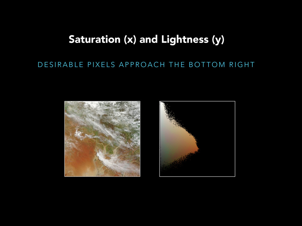
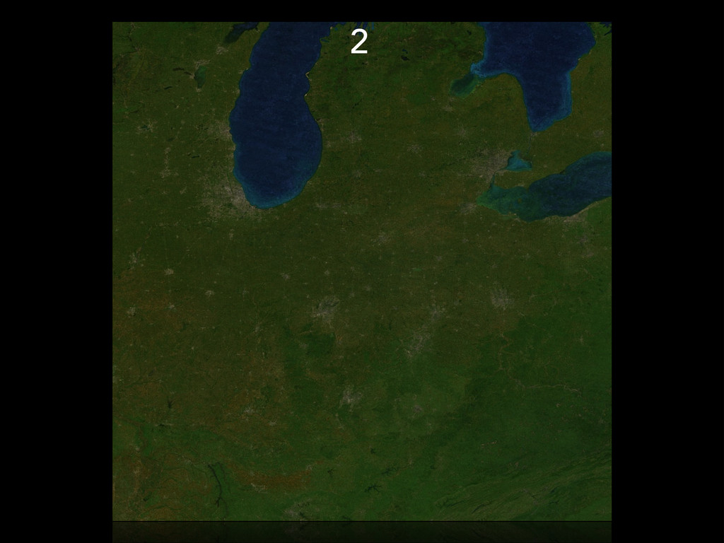
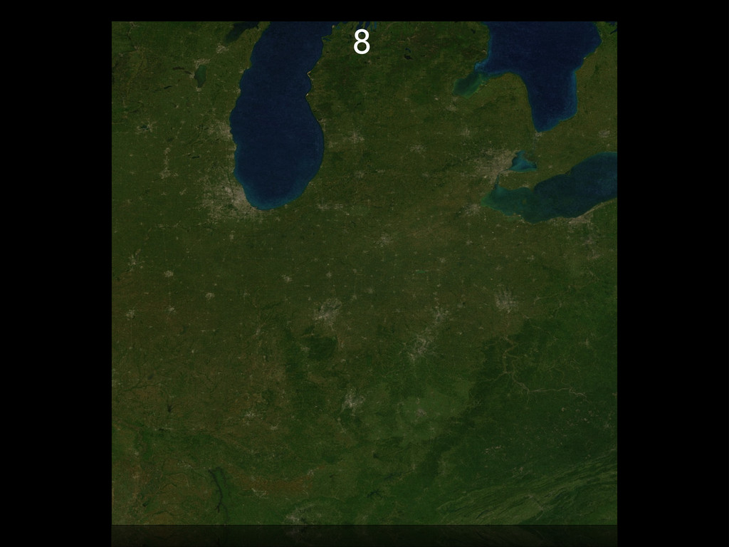
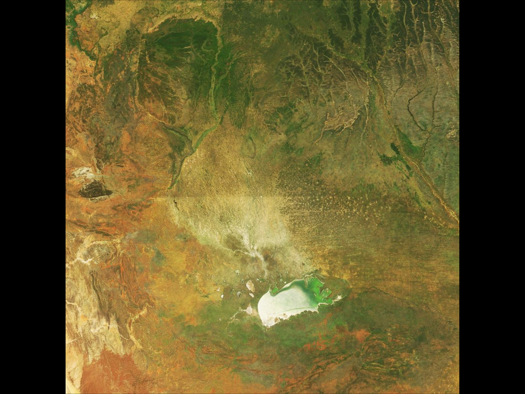
6. Q U A L I T Y • The quality function is the core of this whole process • Algorithm assigns pixels scores based on how much they look like ground cover (as opposed to clouds, smoke, errors, missing data, etc.) • Since it looks at every single input pixel (~5e12 pixels), it has to be very, very simple
7. D E S I R A B L E P I X E L S A P P R O A C H T H E B O T T O M R I G H T ! Saturation (x) and Lightness (y)
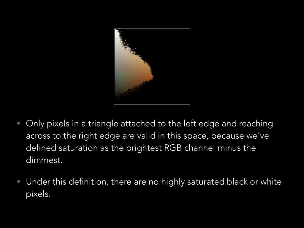
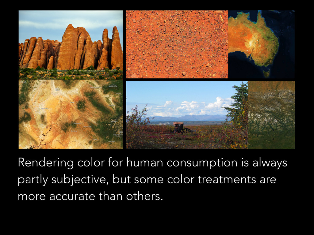
8. • Only pixels in a triangle attached to the left edge and reaching across to the right edge are valid in this space, because we’ve defined saturation as the brightest RGB channel minus the dimmest. • Under this definition, there are no highly saturated black or white pixels.
9. Q U A L I T Y
10. T H E S O RT E D S TA C K
13. 1 3
14. 2 6
15. 4 1
16. 5 8
17. T H E D ATA
19. S O U R C E I M A G E RY • NASA Lance-MODIS Rapid Response 9°×9°s • 374 tiles (row/column subsets overlapping land) • 730–1460 scenes per tile
20. L A N C E M O D I S S U B S E T S
21. E X A M P L E : R O W 1 4 , C O L U M N 1 1 , T E R R A O C T. 1 5 , 2 0 1 2
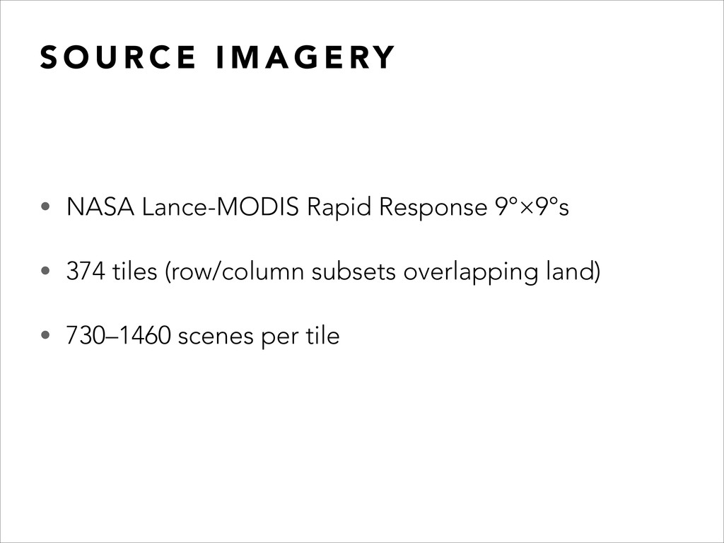
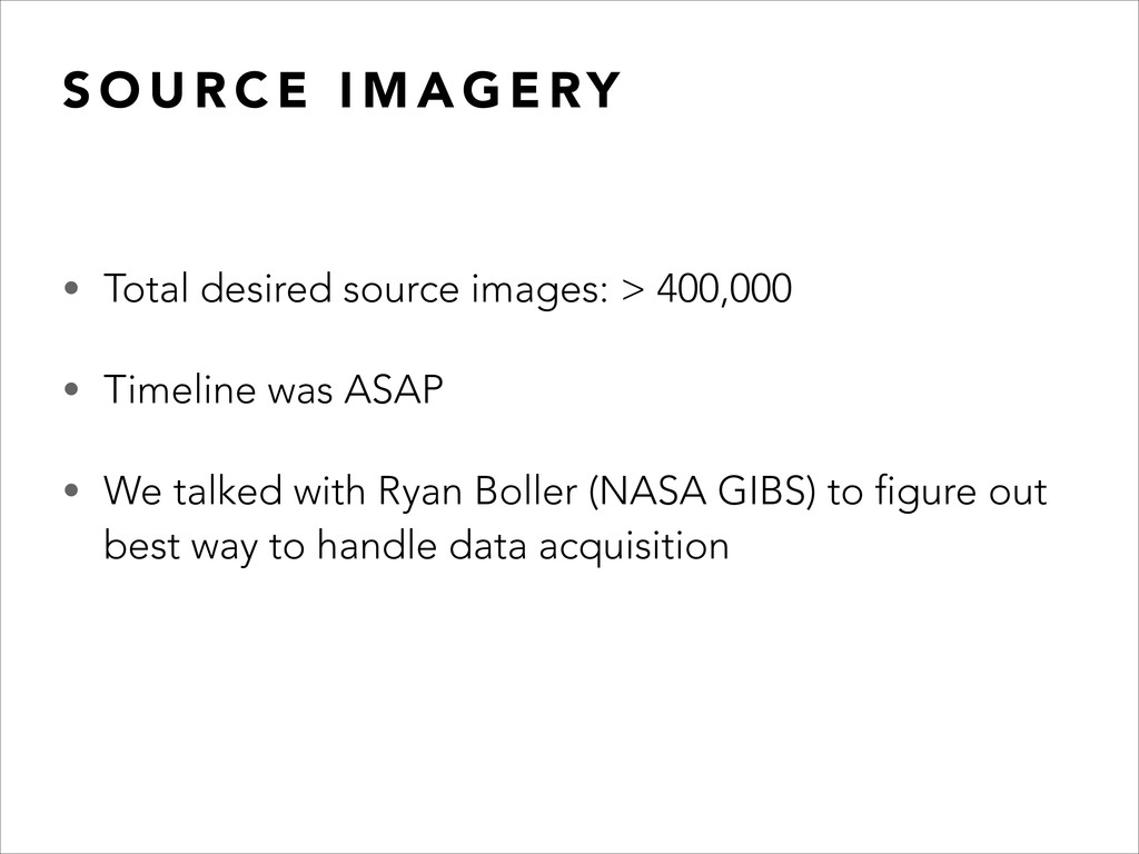
22. S O U R C E I M A G E RY • Total desired source images: > 400,000 • Timeline was ASAP • We talked with Ryan Boller (NASA GIBS) to figure out best way to handle data acquisition
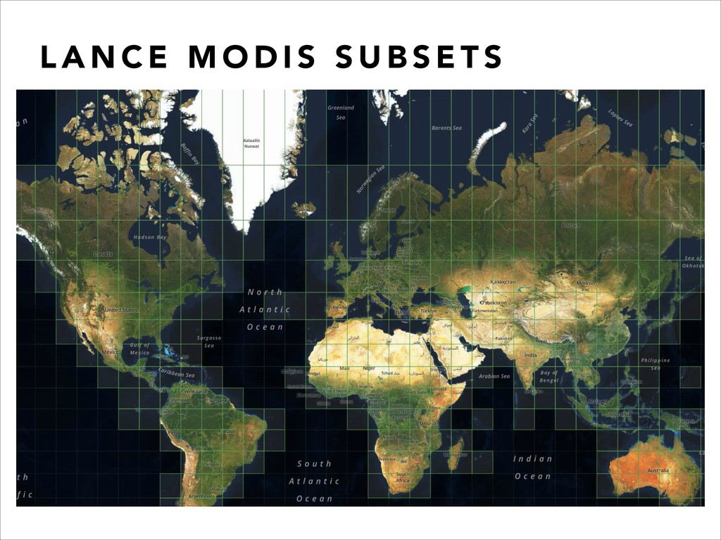
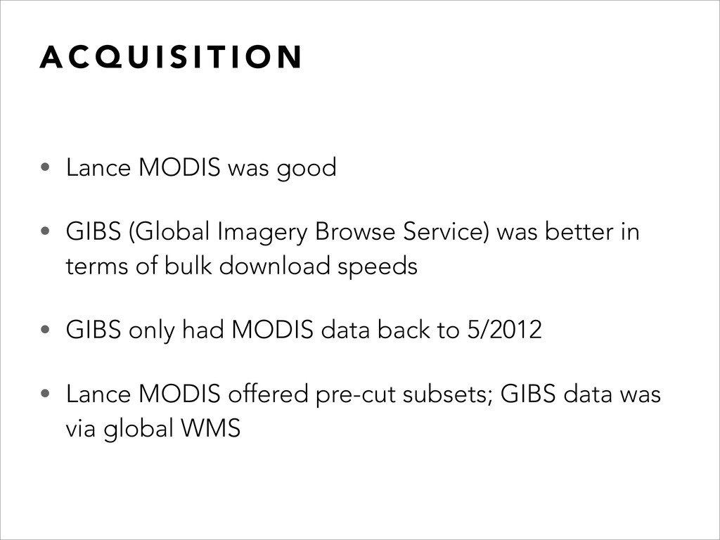
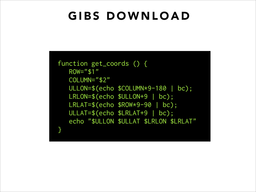
23. A C Q U I S I T I O N • Lance MODIS was good • GIBS (Global Imagery Browse Service) was better in terms of bulk download speeds • GIBS only had MODIS data back to 5/2012 • Lance MODIS offered pre-cut subsets; GIBS data was via global WMS
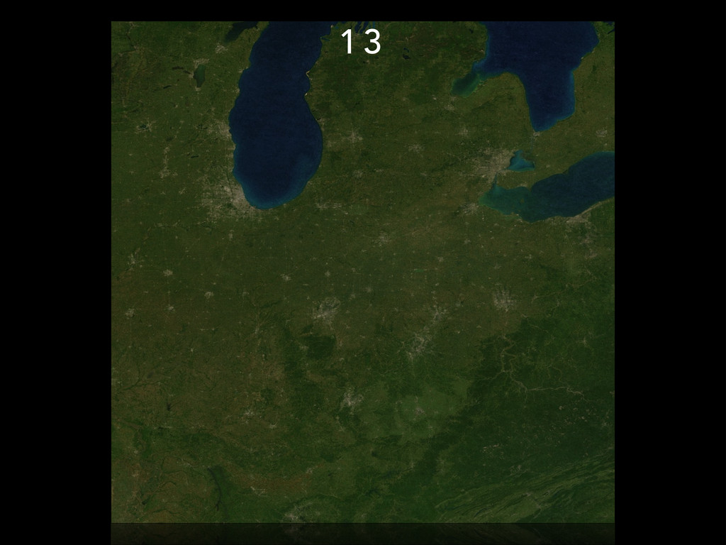
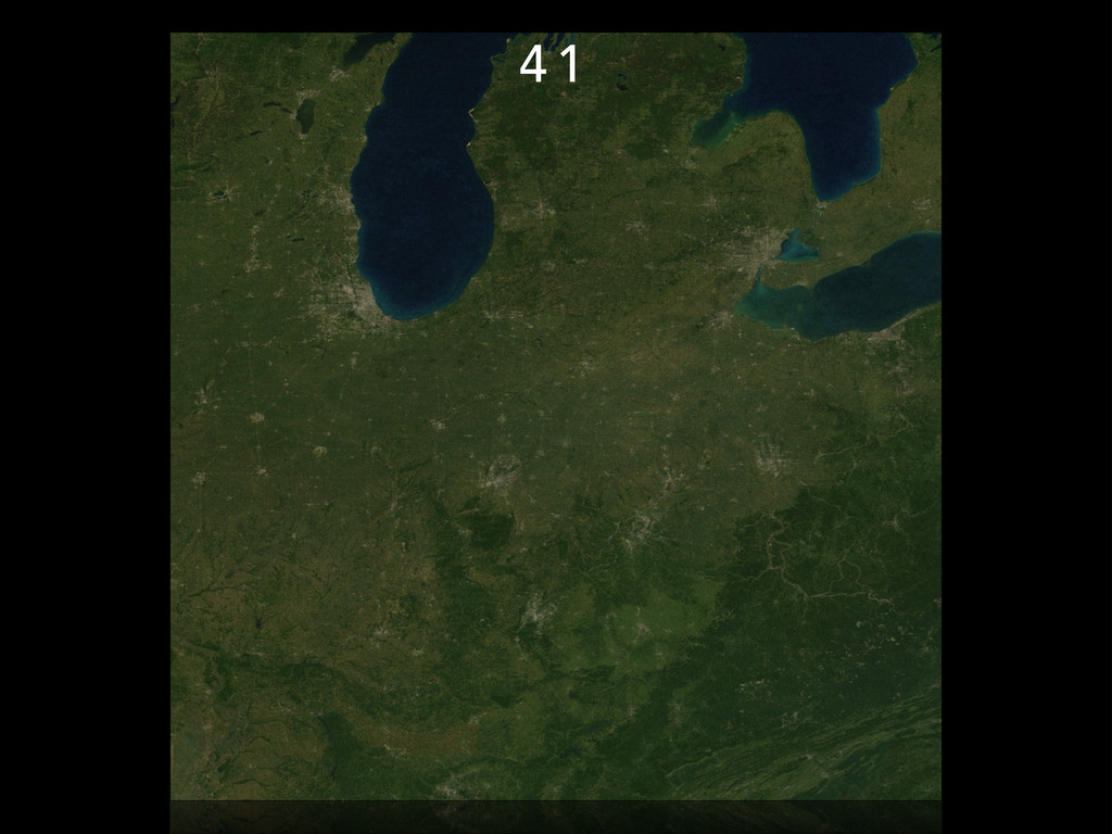
24. D O W N L O A D P L A N • Rows 0–7: days of the year 1–80, 265–366 • Rows 8–11: all days of the year • Rows 12+: days of the year 81–264 • All 2011 imagery from Lance • 2012-001–2012-137 from Lance • 2012-138+ from GIBS
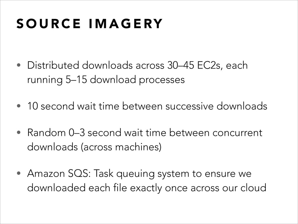
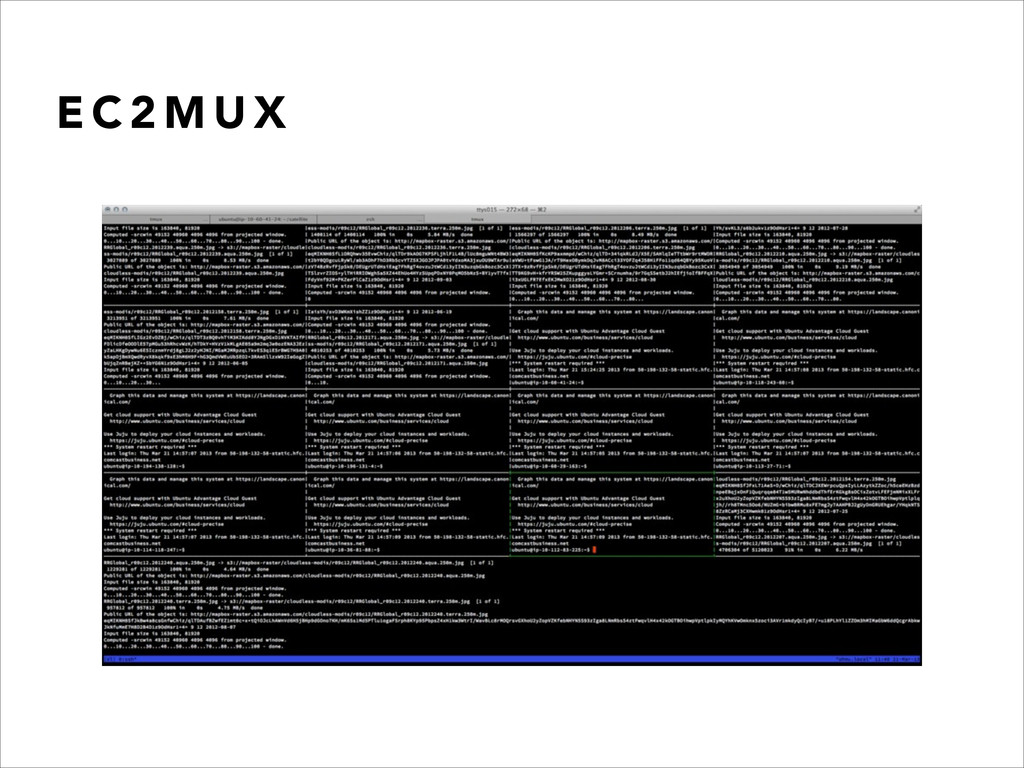
25. S O U R C E I M A G E RY • Distributed downloads across 30–45 EC2s, each running 5–15 download processes • 10 second wait time between successive downloads • Random 0–3 second wait time between concurrent downloads (across machines) • Amazon SQS: Task queuing system to ensure we downloaded each file exactly once across our cloud
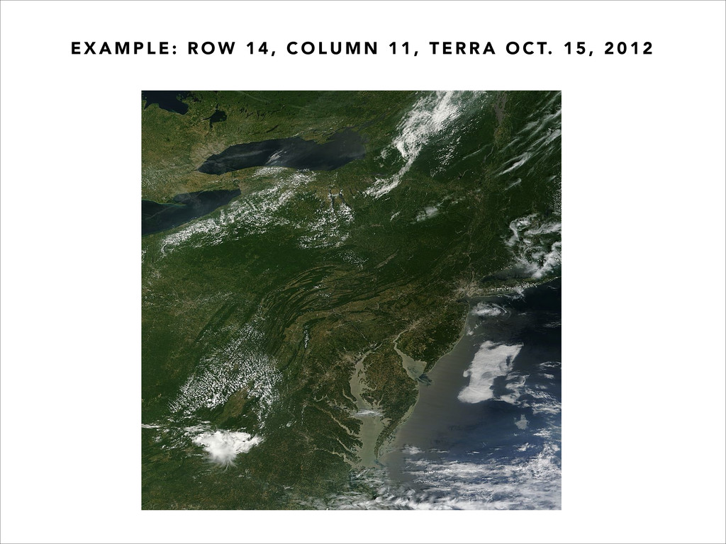
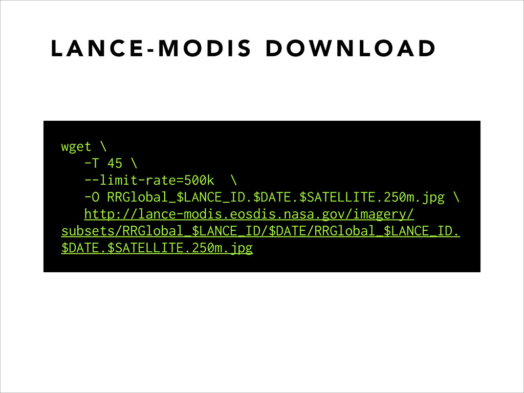
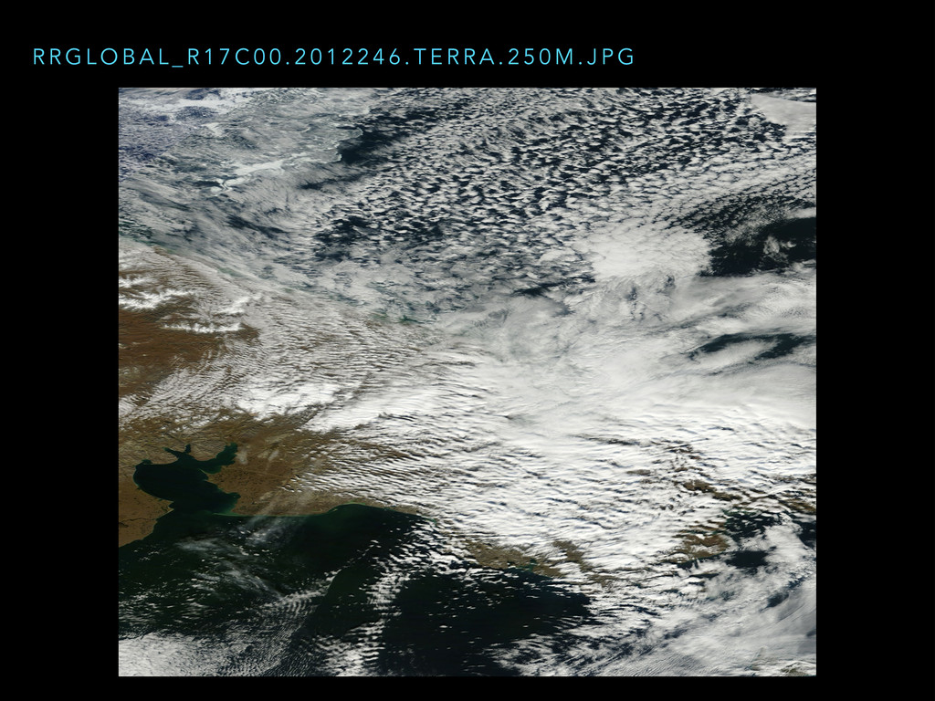
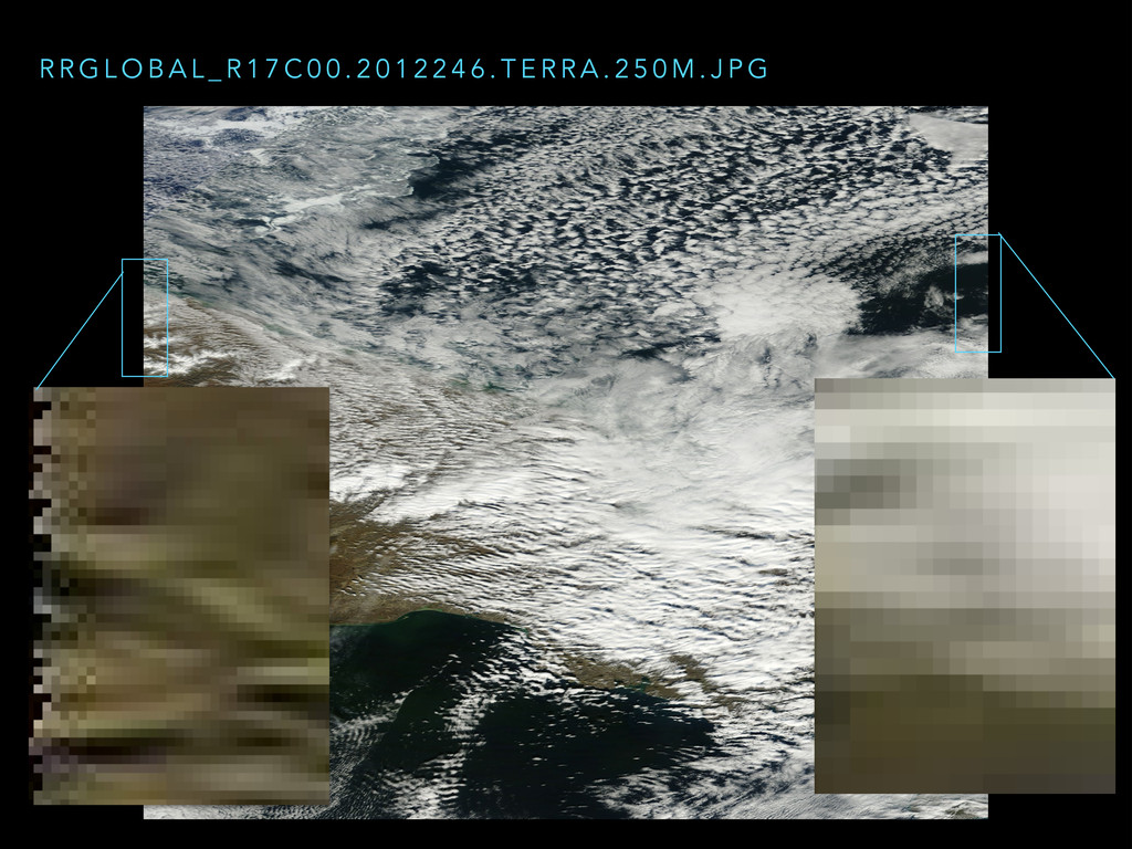
26. wget \ -T 45 \ --limit-rate=500k \ -O RRGlobal_$LANCE_ID.$DATE.$SATELLITE.250m.jpg \ http://lance-modis.eosdis.nasa.gov/imagery/ subsets/RRGlobal_$LANCE_ID/$DATE/RRGlobal_$LANCE_ID. $DATE.$SATELLITE.250m.jpg L A N C E - M O D I S D O W N L O A D
27. function get_coords () { ROW="$1" COLUMN="$2" ULLON=$(echo $COLUMN*9-180 | bc); LRLON=$(echo $ULLON+9 | bc); LRLAT=$(echo $ROW*9-90 | bc); ULLAT=$(echo $LRLAT+9 | bc); echo "$ULLON $ULLAT $LRLON $LRLAT" } G I B S D O W N L O A D
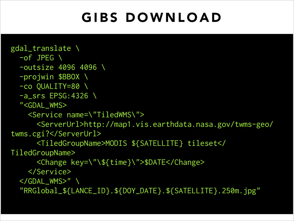
28. gdal_translate \ -of JPEG \ -outsize 4096 4096 \ -projwin $BBOX \ -co QUALITY=80 \ -a_srs EPSG:4326 \ "<GDAL_WMS> <Service name=\"TiledWMS\"> <ServerUrl>http://map1.vis.earthdata.nasa.gov/twms-geo/ twms.cgi?</ServerUrl> <TiledGroupName>MODIS ${SATELLITE} tileset</ TiledGroupName> <Change key=\"\${time}\">$DATE</Change> </Service> </GDAL_WMS>" \ "RRGlobal_${LANCE_ID}.${DOY_DATE}.${SATELLITE}.250m.jpg" G I B S D O W N L O A D
29. P R O C E S S I N G
30. P R O C E S S I N G Declouding for all 374 tiles: 639 computing hours ! 40 Amazon EC2 spot instances (M2.2XL) for 16 hours ! Besides a few tests and re-dos, the bulk of the processing happened over a single weekend.
31. E C 2 M U X
32. E C 2 M U X
33. C H A L L E N G E S
34. D AT E L I N E L O N G I T U D E ± 1 8 0 (That’s an image bug, not a deliberate highlight…)
35. R R G L O B A L _ R 1 7 C 0 0 . 2 0 1 2 2 4 6 . T E R R A . 2 5 0 M . J P G
36. R R G L O B A L _ R 1 7 C 0 0 . 2 0 1 2 2 4 6 . T E R R A . 2 5 0 M . J P G
37. C O L O R
38. Rendering color for human consumption is always partly subjective, but some color treatments are more accurate than others.
39. A N TA R C T I C A
40. D E C L O U D E D A N TA R C T I C A
41. L I M A L A N D S A T I M A G E M O S A I C O F A N TA R C T I C A
42. M O A M O S A I C O F A N TA R C T I C A
43. R E S U LT S
47. A P R E V I E W O F M A P B O X ’ S N E X T I T E R AT I O N O F C L O U D L E S S AT L A S ! T H E C L O U D V. C L O U D S
48. Artist’s Rendering of Landsat 7, Credit: NASA/Goddard
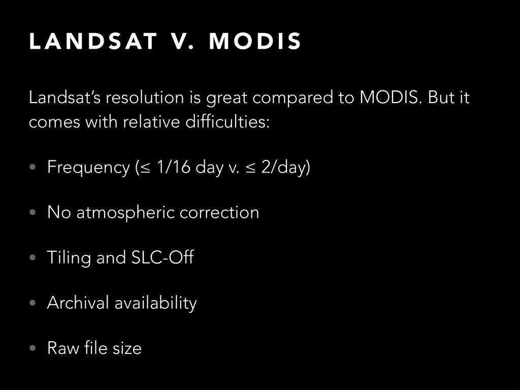
50. L A N D S AT V. M O D I S Landsat’s resolution is great compared to MODIS. But it comes with relative difficulties: • Frequency (≤ 1/16 day v. ≤ 2/day) • No atmospheric correction • Tiling and SLC-Off • Archival availability • Raw file size
51. T I L I N G A N D S L C - O F F Because both are essentially missing data problems, we have a technique: treat null bands and missing corners like clouds!
52. AT M O S P H E R I C C O R R E C T I O N • ~2,000,000 source images meet project specs • That’s a lot of LEDAPS! • 200,000 computing hours for atmospheric correction
53. L E D A P S • High-quality software routines improve L1 images substantially • Not enough documentation easily accessible for use of software/underlying algorithm • No Landsat 8 support (yet) • Compiling is a chore -> AWS Cloudformation + AMIs
54. B E F O R E + A F T E R
55. • Fewer Landsat scenes available • Scene bundles come with a lot of extra info • Sometimes scenes with coverage we want weren’t collected or archived • Solution: multiple endpoints AVA I L A B I L I T Y
56. • Individual MODIS images: 2-3mb • Individual Landsat scenes: 200-300mb S I Z E
57. T O TA L L A N D S AT 5 A N D 7 S C E N E S AVA I L A B L E F R O M U S G S T H AT M E E T P R O J E C T S P E C S : 2 , 4 0 2 , 0 5 6
58. 4 0 0 T B
59. • Did we mention we don’t have an in-house data center or dedicated servers?
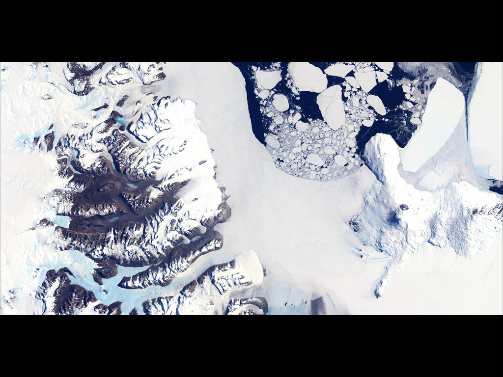
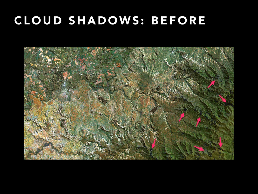
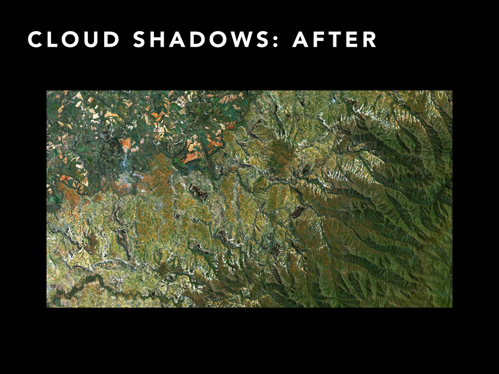
61. C L O U D S H A D O W S Cloud shadows don’t really matter until you’re at about 100 m/px or sharper. ! They trick a naïve algorithm because they’re darker, which usually means clearer, than other pixels. ! So you have to get into fine-tuning the band math, which has other effects too!
62. C L O U D S H A D O W S : B E F O R E
63. C L O U D S H A D O W S : A F T E R
64. W O R K C O N T I N U E S !
65. Q U E S T I O N S ? C O M M E N T S ? Chris Herwig (@hrwgc)
 chris@mapbox.com Charlie Loyd (@vruba)
 charlie@mapbox.com Bruno Sánchez-Andrade Nuño
 (@brunosan) – bruno@mapbox.com