Statistical Learning

Statistical learning theory is a framework for machine learning drawing from the fields of statistics and functional analysis

Transcript

1. Confidential Customized for Lorem Ipsum LLC Version 1.0 Statistical Learning - What, Why and How? Presented By : Mayank Mishra A Data Geek passionate about Artificial Intelligence | Machine Learning Data Science Engineer @ Infostretch
2. Confidential Customized for Lorem Ipsum LLC Version 1.0 Line Up Objective Why statistical Learning How to estimate f ? Quality of Fit Bias Variance Trade Off
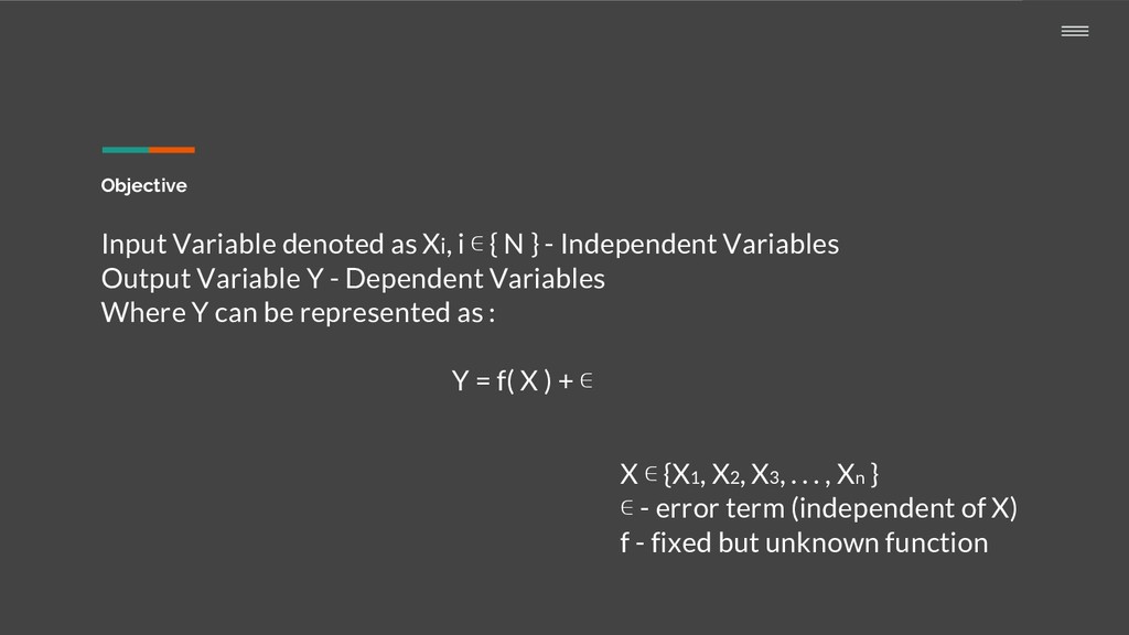
3. Objective Input Variable denoted as Xi, i ∊ { N } - Independent Variables Output Variable Y - Dependent Variables Where Y can be represented as : Y = f( X ) + ∊ X ∊ {X1, X2, X3, . . . , Xn } ∊ - error term (independent of X) f - fixed but unknown function
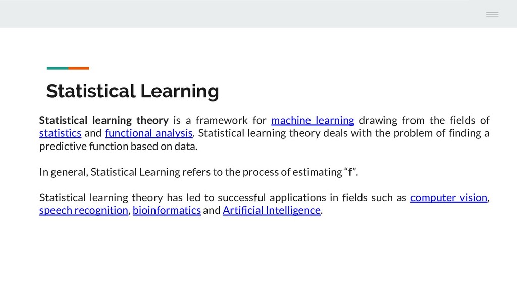
4. Statistical Learning Statistical learning theory is a framework for machine learning drawing from the fields of statistics and functional analysis. Statistical learning theory deals with the problem of finding a predictive function based on data. In general, Statistical Learning refers to the process of estimating “f”. Statistical learning theory has led to successful applications in fields such as computer vision, speech recognition, bioinformatics and Artificial Intelligence.
5. Why ??
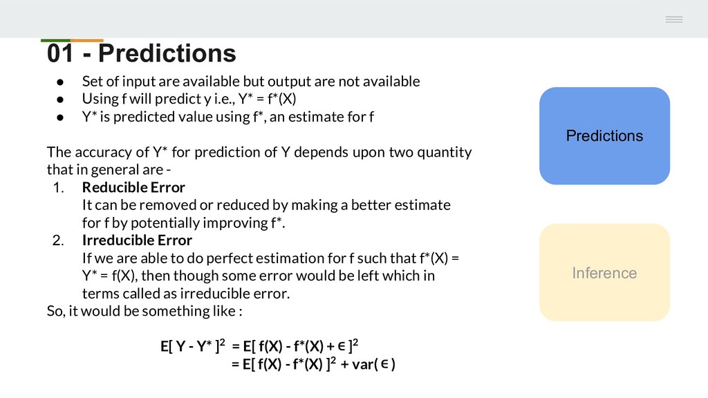
6. 01 - Predictions Predictions Inference • Set of input are available but output are not available • Using f will predict y i.e., Y* = f*(X) • Y* is predicted value using f*, an estimate for f The accuracy of Y* for prediction of Y depends upon two quantity that in general are - 1. Reducible Error It can be removed or reduced by making a better estimate for f by potentially improving f*. 2. Irreducible Error If we are able to do perfect estimation for f such that f*(X) = Y* = f(X), then though some error would be left which in terms called as irreducible error. So, it would be something like : E[ Y - Y* ]2 = E[ f(X) - f*(X) + ∊ ]2 = E[ f(X) - f*(X) ]2 + var( ∊ )
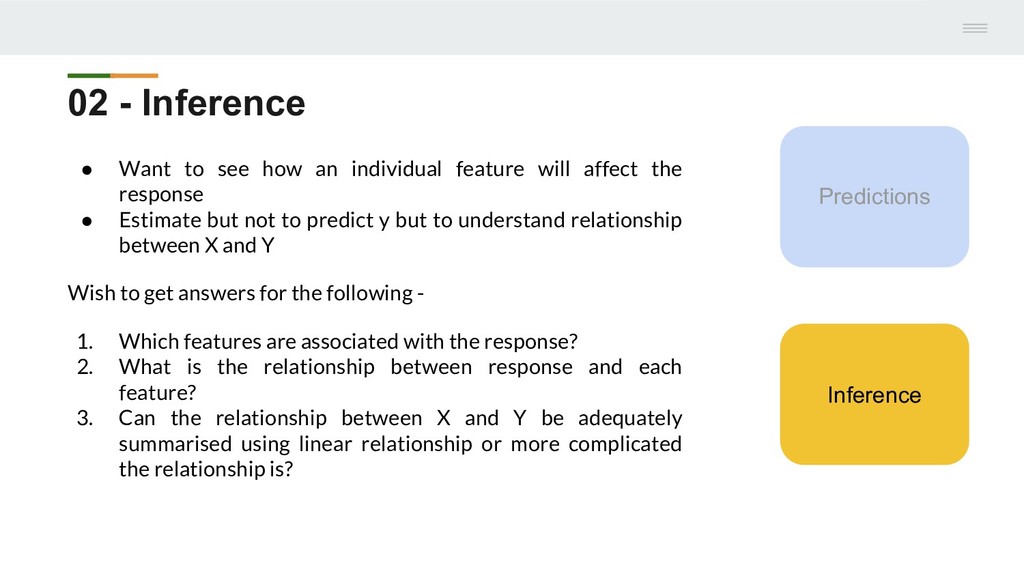
7. 02 - Inference • Want to see how an individual feature will affect the response • Estimate but not to predict y but to understand relationship between X and Y Wish to get answers for the following - 1. Which features are associated with the response? 2. What is the relationship between response and each feature? 3. Can the relationship between X and Y be adequately summarised using linear relationship or more complicated the relationship is? Predictions Inference
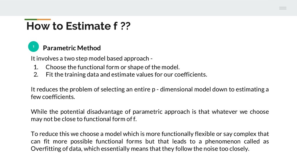
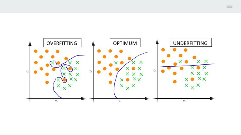
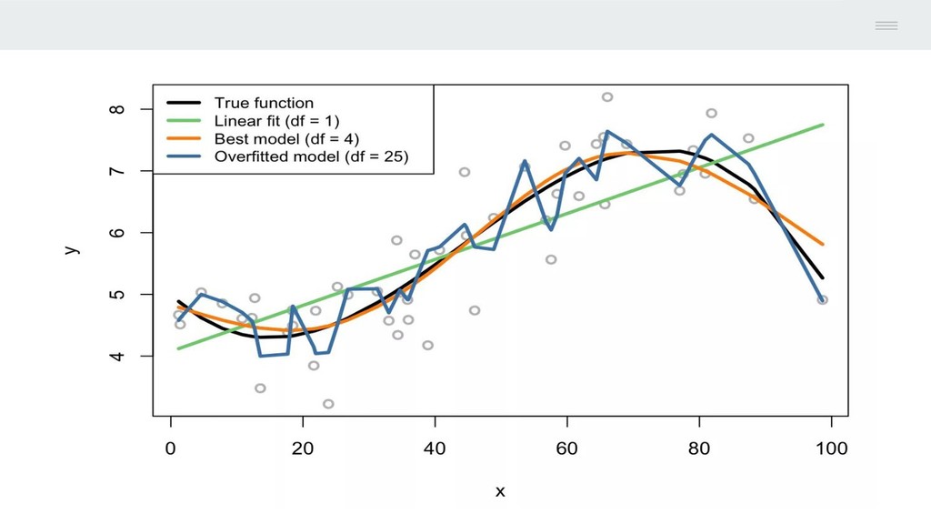
8. It involves a two step model based approach - 1. Choose the functional form or shape of the model. 2. Fit the training data and estimate values for our coefficients. It reduces the problem of selecting an entire p - dimensional model down to estimating a few coefficients. While the potential disadvantage of parametric approach is that whatever we choose may not be close to functional form of f. To reduce this we choose a model which is more functionally flexible or say complex that can fit more possible functional forms but that leads to a phenomenon called as Overfitting of data, which essentially means that they follow the noise too closely. How to Estimate f ?? 1 Parametric Method
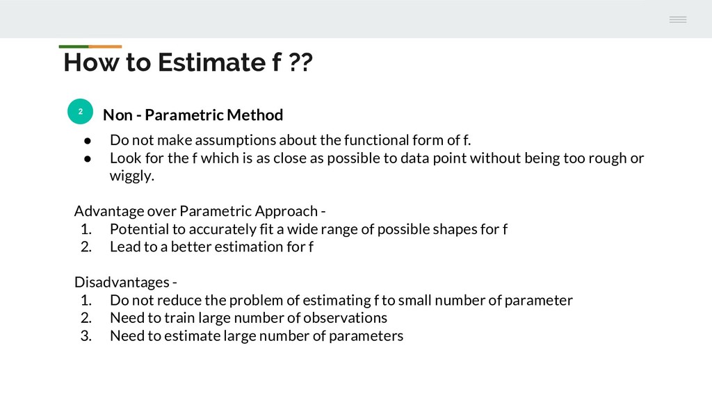
9. • Do not make assumptions about the functional form of f. • Look for the f which is as close as possible to data point without being too rough or wiggly. Advantage over Parametric Approach - 1. Potential to accurately fit a wide range of possible shapes for f 2. Lead to a better estimation for f Disadvantages - 1. Do not reduce the problem of estimating f to small number of parameter 2. Need to train large number of observations 3. Need to estimate large number of parameters How to Estimate f ?? 2 Non - Parametric Method
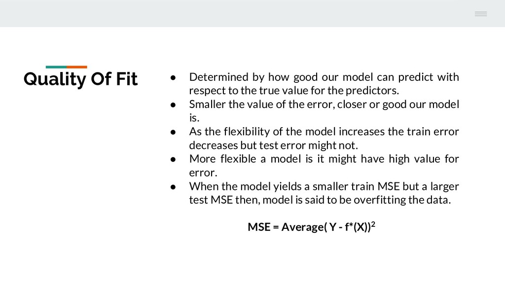
10. Quality Of Fit • Determined by how good our model can predict with respect to the true value for the predictors. • Smaller the value of the error, closer or good our model is. • As the flexibility of the model increases the train error decreases but test error might not. • More flexible a model is it might have high value for error. • When the model yields a smaller train MSE but a larger test MSE then, model is said to be overfitting the data. MSE = Average( Y - f*(X))2
11. Variance The amount by which the f* would changed if we trained it using a different dataset. A method have high variance then small change in training dataset can leads to a larger change in the f*. More flexible model have high variance. • Low Variance: Suggests small changes to the estimate of the target function with changes to the training dataset. Example of low variance algorithm: Linear Regression, LDA and Logistic Regression. • High Variance (Overfitting): Suggests large changes to the estimate of the target function with changes to the training dataset. Example of high variance algorithm: Decision Trees, kNN and SVM.
12. Bias Means how far off our predictions are from real values. Generally parametric algorithms have a high bias making them fast to learn and easier to understand but generally less flexible. In turn they are have lower predictive performance on complex problems that fail to meet the simplifying assumptions of the algorithms bias. • Low Bias: Suggests more assumptions about the form of the target function. Example of low bias algorithms: Decision Trees, kNN and SVM • High-Bias (Underfitting): Suggests less assumptions about the form of the target function. Example of high bias algorithms: Linear Regression, LDA and Logistic Regression.
16. Bias - Variance Trade Off
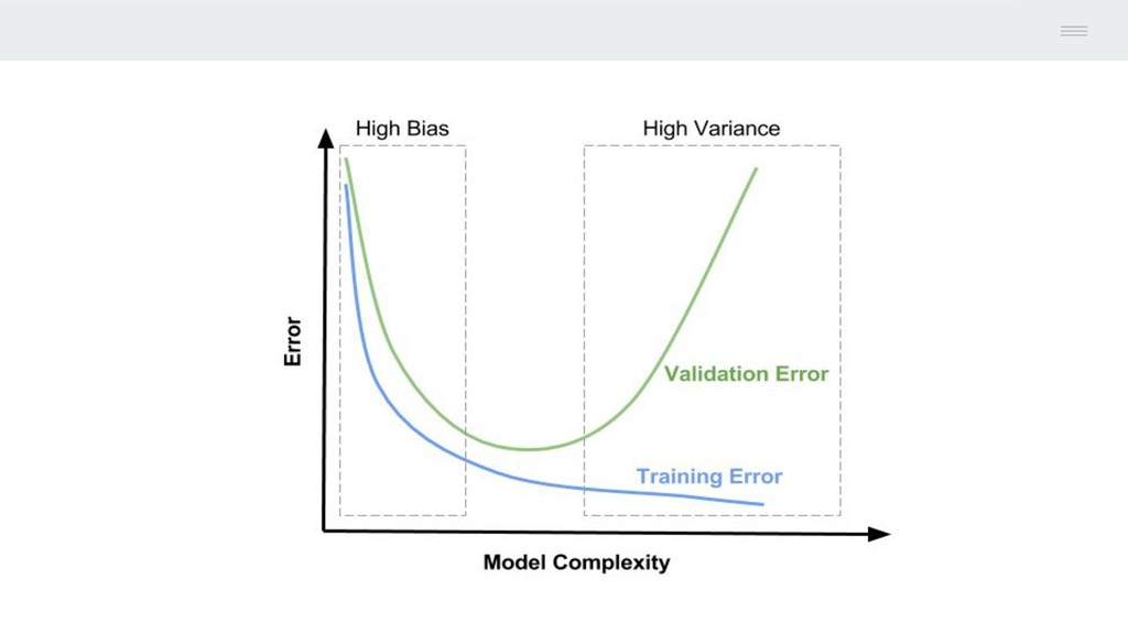
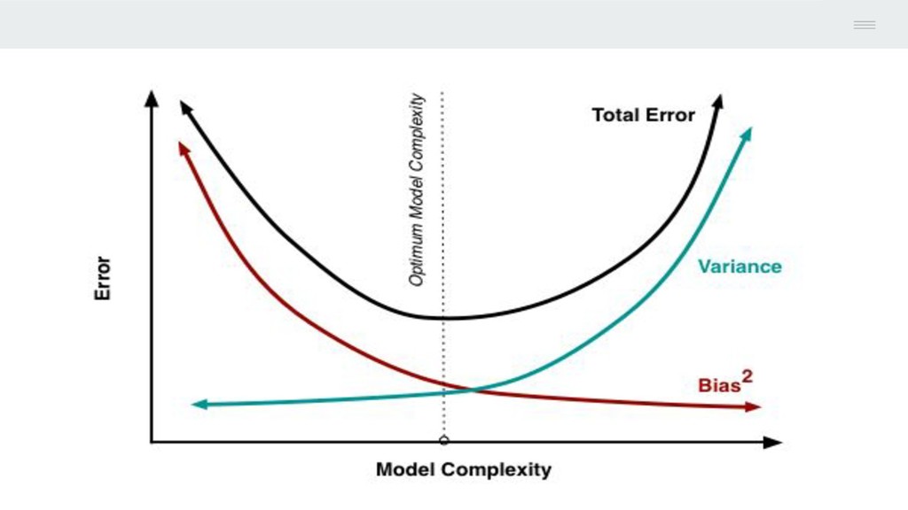
17. Bias-Variance Trade-Off The goal of any supervised machine learning algorithm is to achieve low bias and low variance. In turn the algorithm should achieve good prediction performance. You can see a general trend : • Parametric or linear machine learning algorithms often have a high bias but a low variance. • Non-parametric or non-linear machine learning algorithms often have a low bias but a high variance. The parameterization of machine learning algorithms is often a battle to balance out bias and variance.
18. Bias-Variance Trade-Off Examples of configuring the bias-variance trade-off for specific algorithms: The k-nearest neighbors algorithm has low bias and high variance, but the trade-off can be changed by increasing the value of k which increases the number of neighbors that contribute t the prediction and in turn increases the bias of the model.
19. Bias-Variance Trade-Off There is no escaping the relationship between bias and variance in machine learning. • Increasing the bias will decrease the variance. • Increasing the variance will decrease the bias. There is a trade-off at play between these two concerns and the algorithms you choose and the way you choose to configure them are finding different balances in this trade-off for your problem
21. Thank you. Find me here mayank_skb mayankskb