RTCA Dr Jenny Stocker - The use of monitoring to improve emissions estimates

Transcript

1. Jenny Stocker Routes to Clean Air 2026 Birmingham Routes to Clean Air 2026
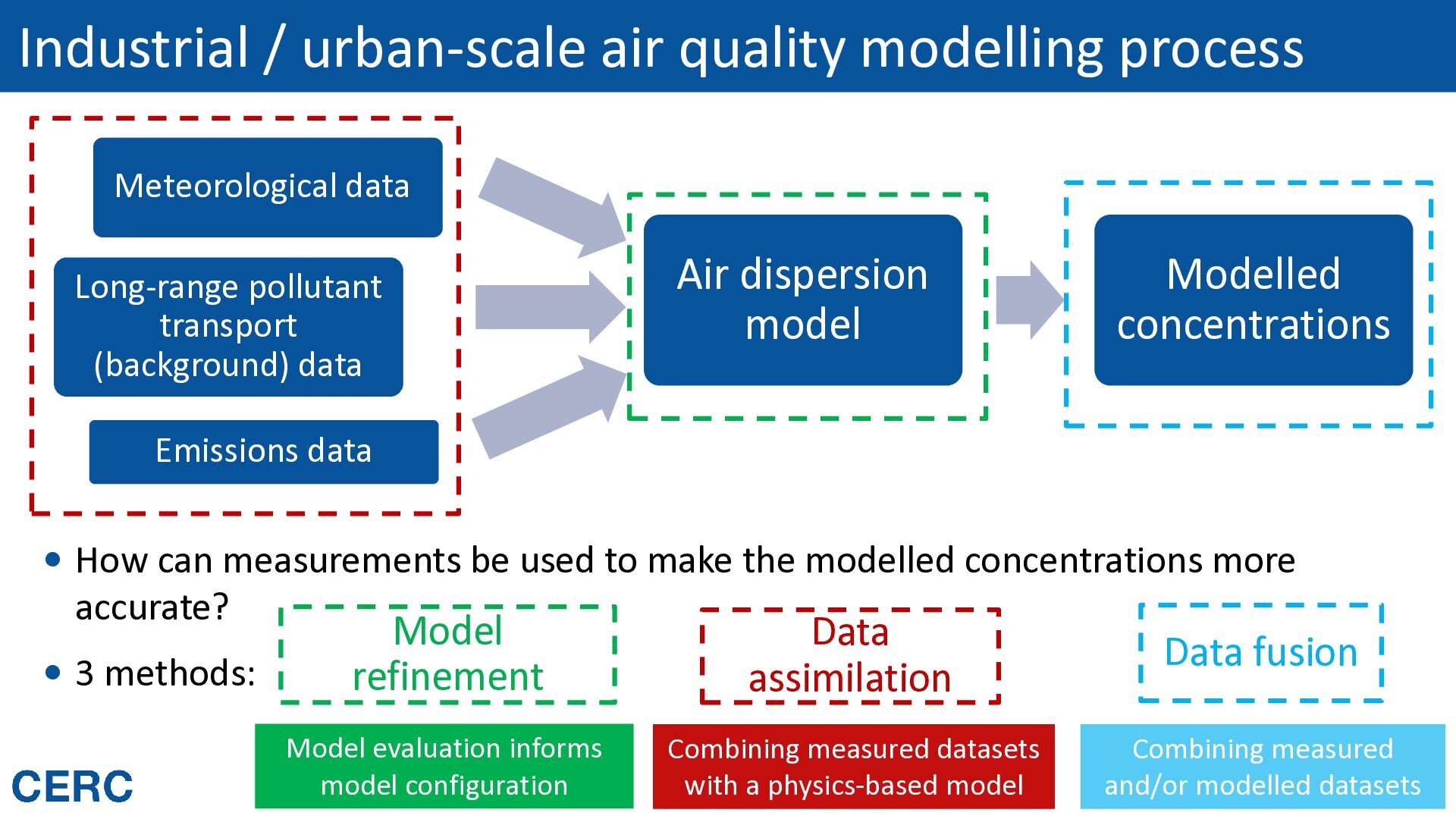
2. Industrial / urban-scale air quality modelling process Meteorological data Long-range pollutant transport (background) data Air dispersion model Modelled concentrations Emissions data  How can measurements be used to make the modelled concentrations more accurate?  3 methods: Model refinement Data assimilation Data fusion Model evaluation informs model configuration Combining measured datasets with a physics-based model Combining measured Routes to Clean Air 2026 and/or modelled datasets
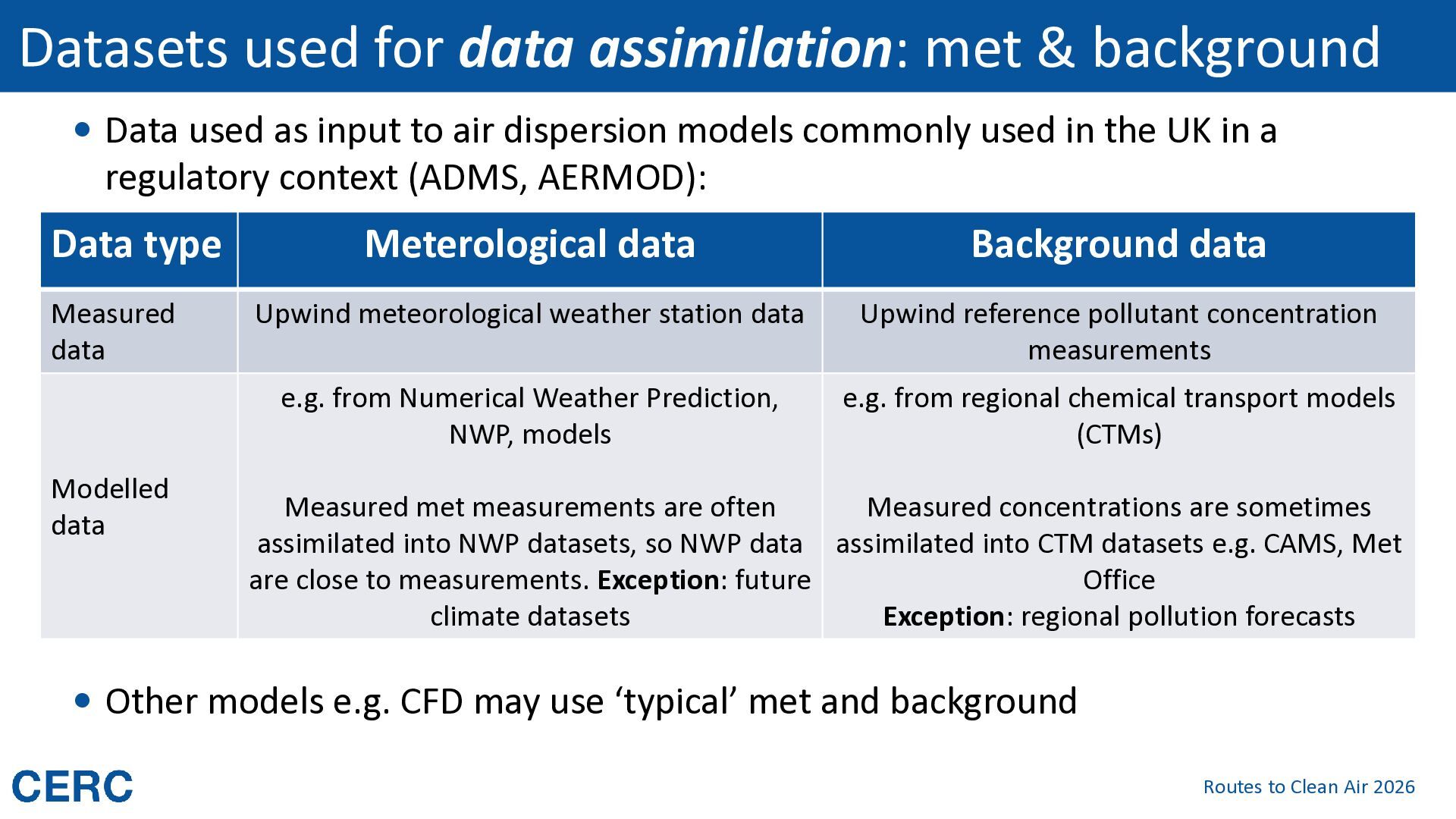
3. Datasets used for data assimilation: met & background  Data used as input to air dispersion models commonly used in the UK in a regulatory context (ADMS, AERMOD): Data type Measured data Modelled data Meterological data Background data Upwind meteorological weather station data Upwind reference pollutant concentration measurements e.g. from Numerical Weather Prediction, NWP, models e.g. from regional chemical transport models (CTMs) Measured met measurements are often Measured concentrations are sometimes assimilated into NWP datasets, so NWP data assimilated into CTM datasets e.g. CAMS, Met are close to measurements. Exception: future Office climate datasets Exception: regional pollution forecasts  Other models e.g. CFD may use ‘typical’ met and background Routes to Clean Air 2026
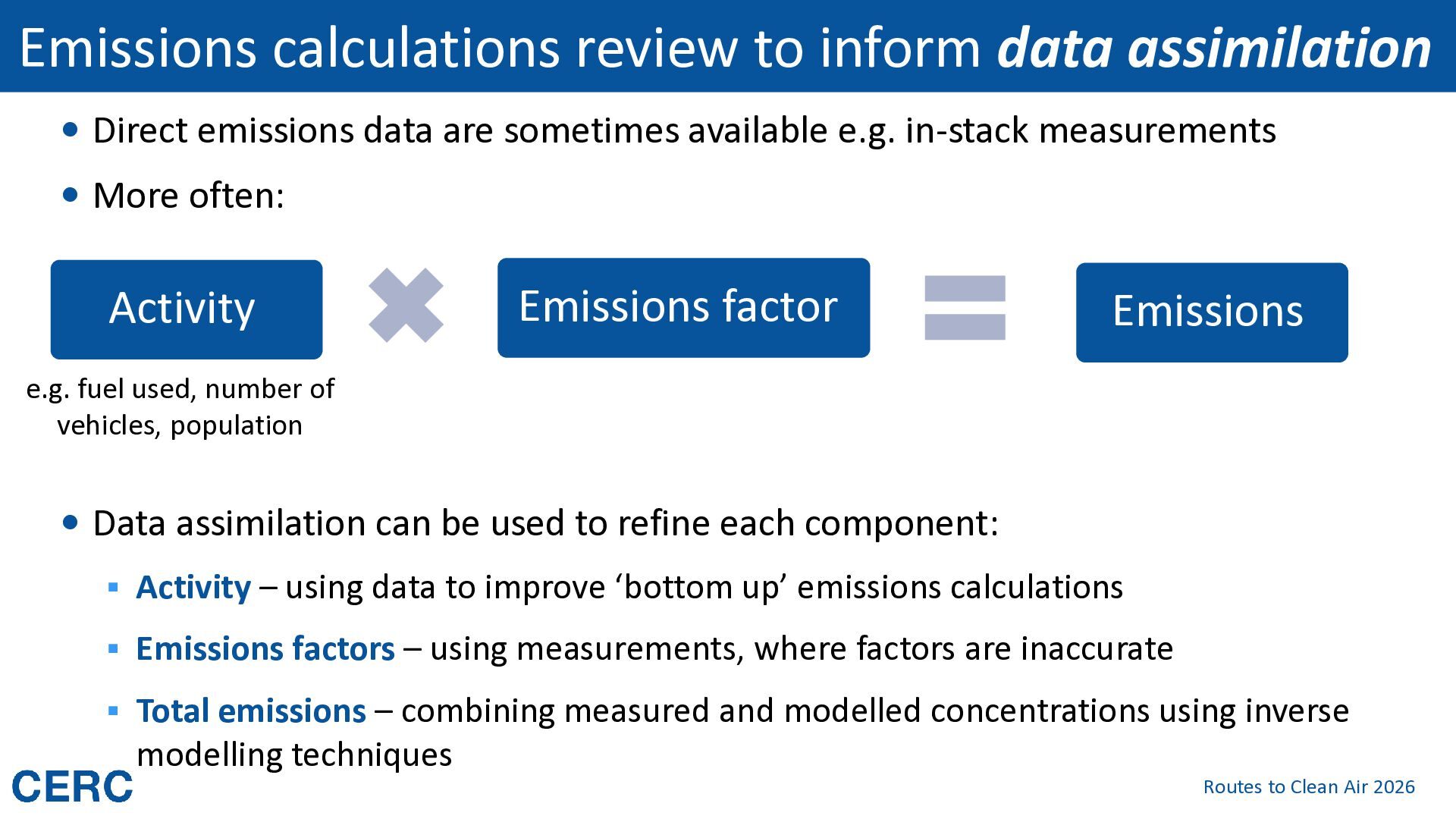
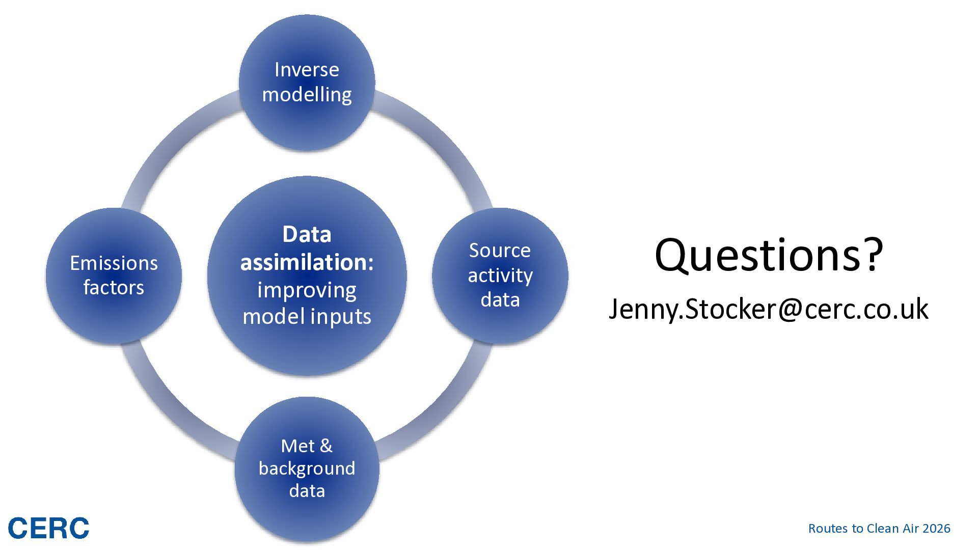
4. Emissions calculations review to inform data assimilation  Direct emissions data are sometimes available e.g. in-stack measurements  More often: Activity Emissions factor Emissions e.g. fuel used, number of vehicles, population  Data assimilation can be used to refine each component: ▪ Activity – using data to improve ‘bottom up’ emissions calculations ▪ Emissions factors – using measurements, where factors are inaccurate ▪ Total emissions – combining measured and modelled concentrations using inverse modelling techniques Routes to Clean Air 2026
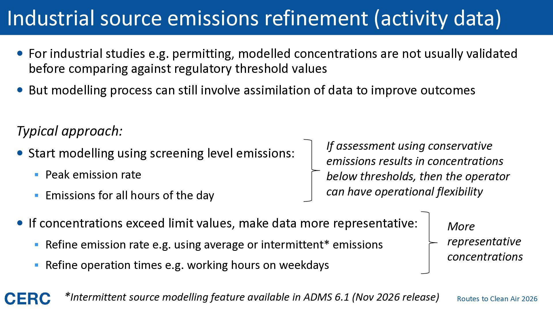
5. Industrial source emissions refinement (activity data)  For industrial studies e.g. permitting, modelled concentrations are not usually validated before comparing against regulatory threshold values  But modelling process can still involve assimilation of data to improve outcomes Typical approach:  Start modelling using screening level emissions: ▪ Peak emission rate ▪ Emissions for all hours of the day If assessment using conservative emissions results in concentrations below thresholds, then the operator can have operational flexibility  If concentrations exceed limit values, make data more representative: ▪ Refine emission rate e.g. using average or intermittent* emissions ▪ Refine operation times e.g. working hours on weekdays *Intermittent source modelling feature available in ADMS 6.1 (Nov 2026 release) More representative concentrations Routes to Clean Air 2026
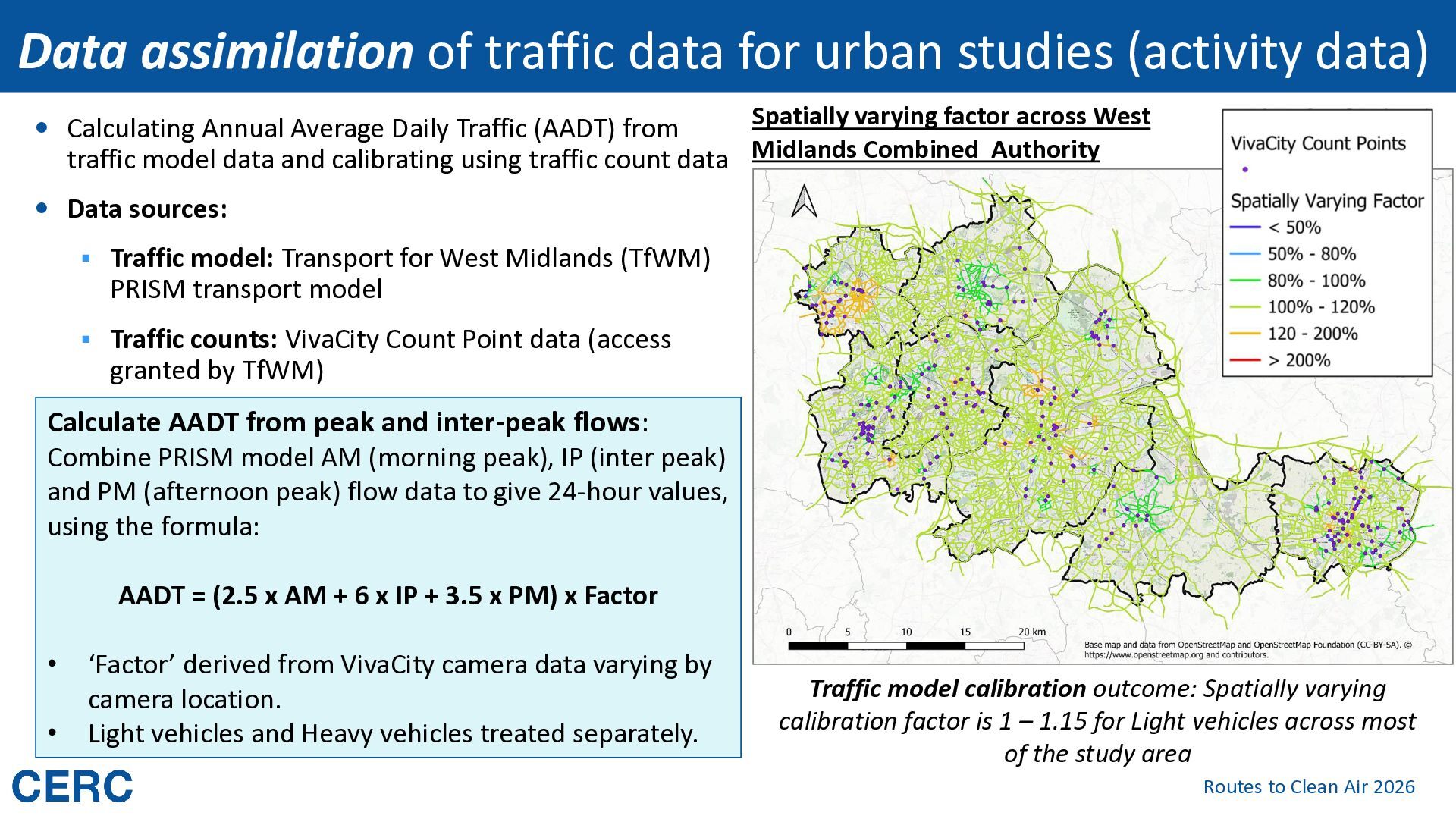
6. Data assimilation of traffic data for urban studies (activity data) Spatially varying factor across West traffic model data and calibrating using traffic count data Midlands Combined Authority  Calculating Annual Average Daily Traffic (AADT) from  Data sources: ▪ Traffic model: Transport for West Midlands (TfWM) PRISM transport model ▪ Traffic counts: VivaCity Count Point data (access granted by TfWM) Calculate AADT from peak and inter-peak flows: Combine PRISM model AM (morning peak), IP (inter peak) and PM (afternoon peak) flow data to give 24-hour values, using the formula: AADT = (2.5 x AM + 6 x IP + 3.5 x PM) x Factor • • ‘Factor’ derived from VivaCity camera data varying by camera location. Light vehicles and Heavy vehicles treated separately. Traffic model calibration outcome: Spatially varying calibration factor is 1 – 1.15 for Light vehicles across most of the study area Routes to Clean Air 2026
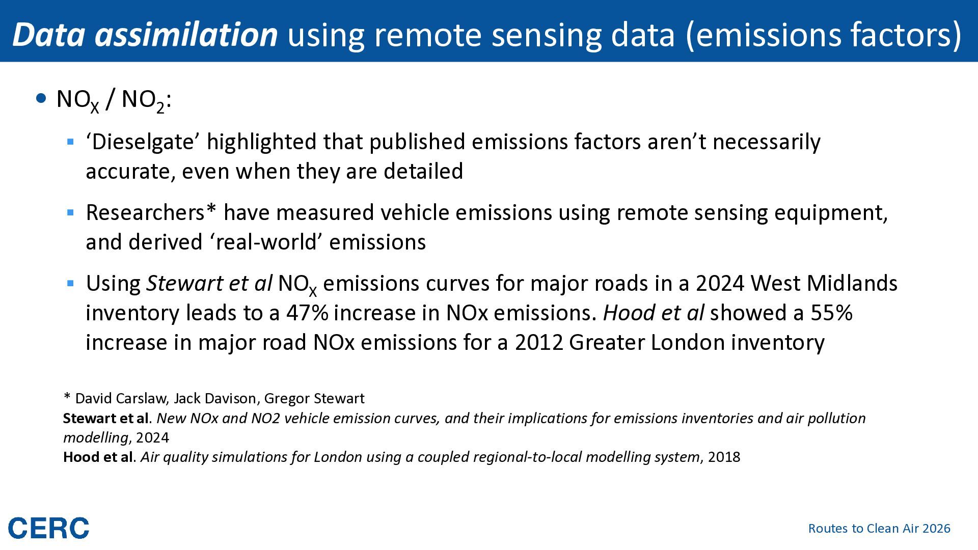
7. Data assimilation using remote sensing data (emissions factors)  NOX / NO2: ▪ ‘Dieselgate’ highlighted that published emissions factors aren’t necessarily accurate, even when they are detailed ▪ Researchers* have measured vehicle emissions using remote sensing equipment, and derived ‘real-world’ emissions ▪ Using Stewart et al NOX emissions curves for major roads in a 2024 West Midlands inventory leads to a 47% increase in NOx emissions. Hood et al showed a 55% increase in major road NOx emissions for a 2012 Greater London inventory * David Carslaw, Jack Davison, Gregor Stewart Stewart et al. New NOx and NO2 vehicle emission curves, and their implications for emissions inventories and air pollution modelling, 2024 Hood et al. Air quality simulations for London using a coupled regional-to-local modelling system, 2018 Routes to Clean Air 2026
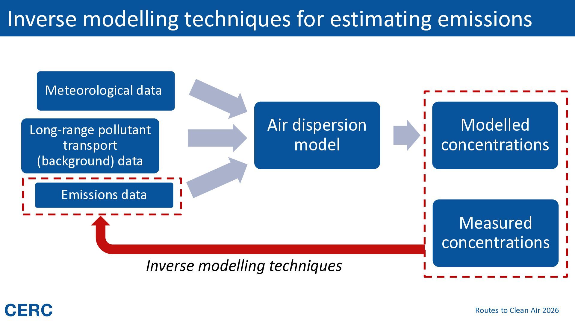
8. Inverse modelling techniques for estimating emissions Meteorological data Long-range pollutant transport (background) data Air dispersion model Modelled concentrations Emissions data Measured concentrations Inverse modelling techniques Routes to Clean Air 2026
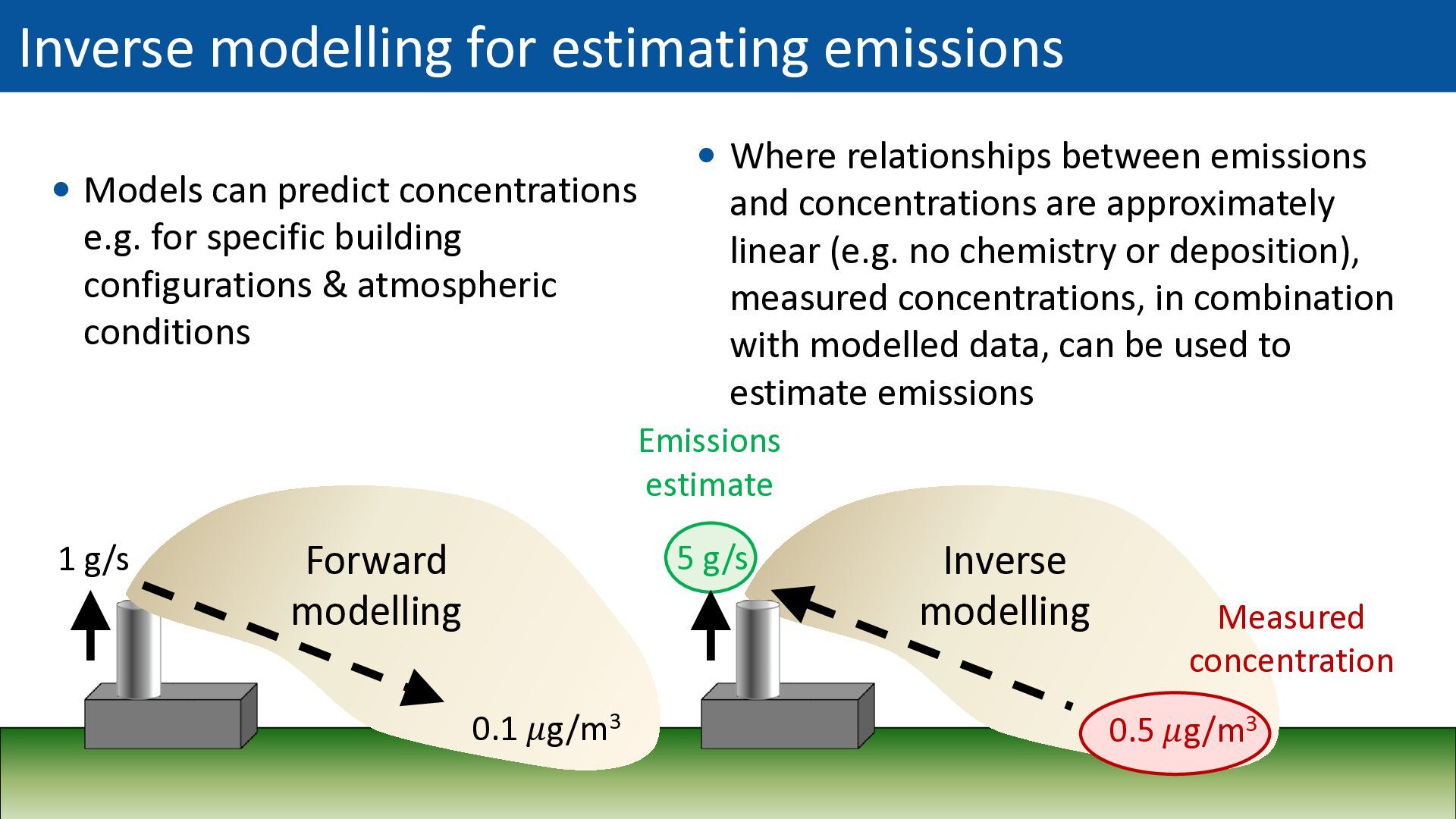
9. Inverse modelling for estimating emissions  Models can predict concentrations e.g. for specific building configurations & atmospheric conditions  Where relationships between emissions and concentrations are approximately linear (e.g. no chemistry or deposition), measured concentrations, in combination with modelled data, can be used to estimate emissions Emissions estimate 1 g/s Forward modelling 5 g/s 0.1 𝜇g/m3 Inverse modelling Measured concentration 0.5 𝜇g/m3 Routes to Clean Air 2026
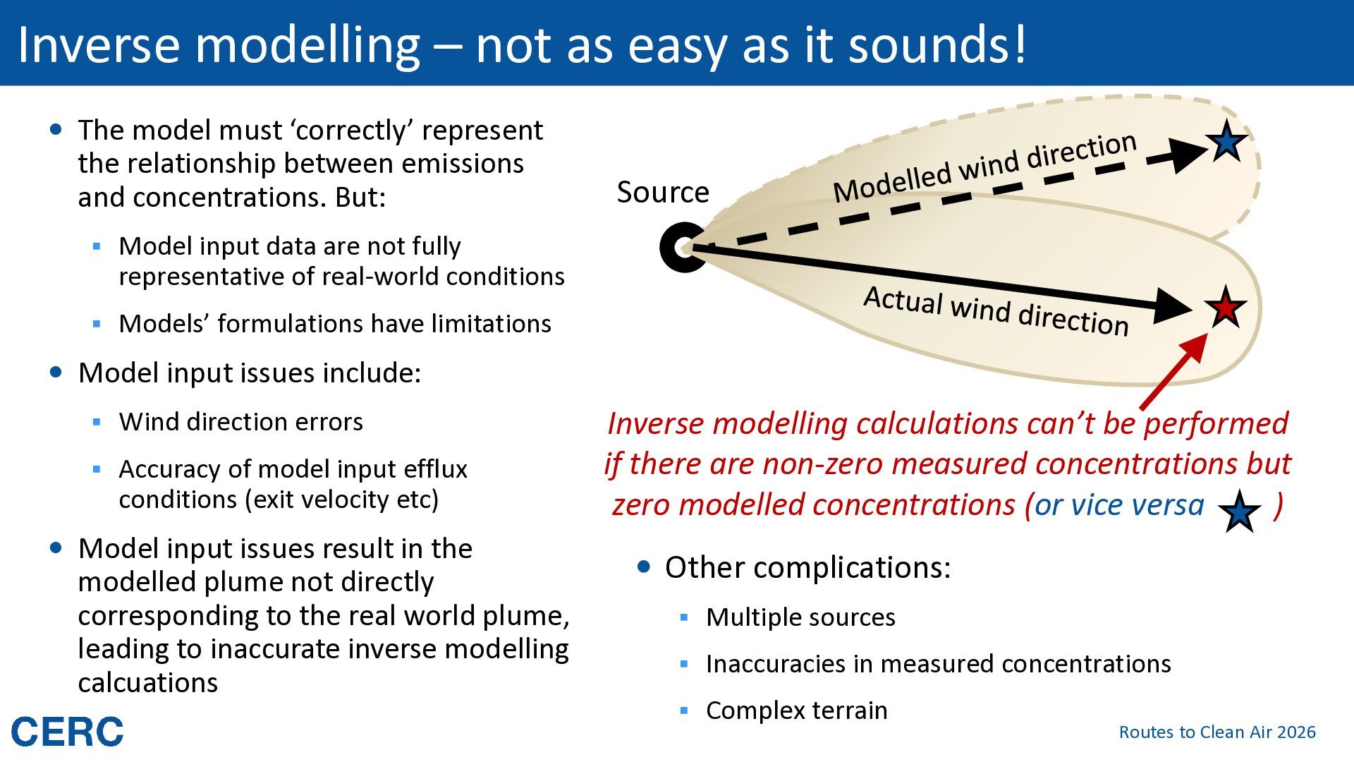
10. Inverse modelling – not as easy as it sounds!  The model must ‘correctly’ represent the relationship between emissions and concentrations. But: Source ▪ Model input data are not fully representative of real-world conditions ▪ Models’ formulations have limitations  Model input issues include: ▪ Wind direction errors ▪ Accuracy of model input efflux conditions (exit velocity etc)  Model input issues result in the modelled plume not directly corresponding to the real world plume, leading to inaccurate inverse modelling calcuations Inverse modelling calculations can’t be performed if there are non-zero measured concentrations but zero modelled concentrations (or vice versa )  Other complications: ▪ Multiple sources ▪ Inaccuracies in measured concentrations ▪ Complex terrain Routes to Clean Air 2026
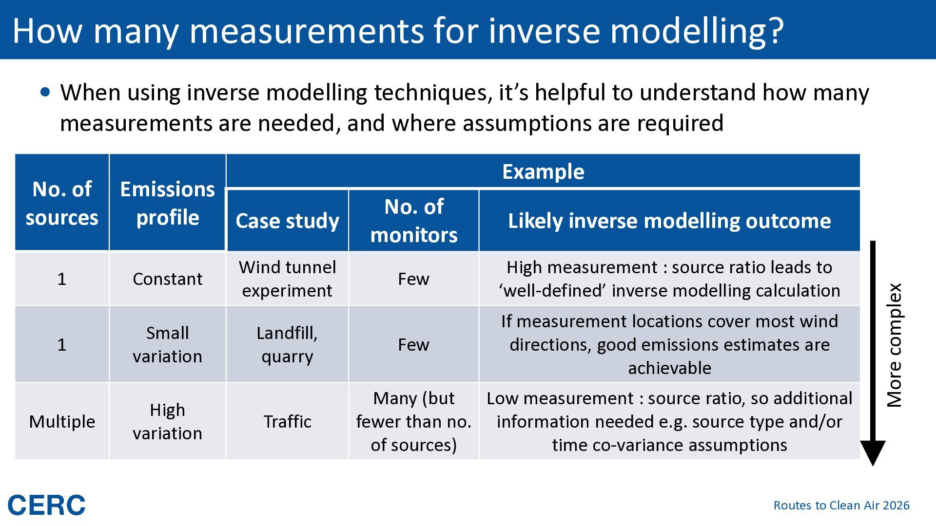
11. How many measurements for inverse modelling?  When using inverse modelling techniques, it’s helpful to understand how many measurements are needed, and where assumptions are required 1 Constant Wind tunnel experiment 1 Small variation Landfill, quarry Multiple High variation Traffic No. of monitors Likely inverse modelling outcome Few High measurement : source ratio leads to ‘well-defined’ inverse modelling calculation Few If measurement locations cover most wind directions, good emissions estimates are achievable Many (but Low measurement : source ratio, so additional fewer than no. information needed e.g. source type and/or of sources) time co-variance assumptions More complex No. of Emissions sources profile Case study Example Routes to Clean Air 2026
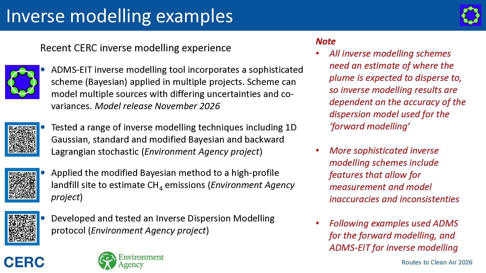
12. Inverse modelling examples Recent CERC inverse modelling experience  ADMS-EIT inverse modelling tool incorporates a sophisticated scheme (Bayesian) applied in multiple projects. Scheme can model multiple sources with differing uncertainties and covariances. Model release November 2026  Tested a range of inverse modelling techniques including 1D Gaussian, standard and modified Bayesian and backward Lagrangian stochastic (Environment Agency project) Note • All inverse modelling schemes need an estimate of where the plume is expected to disperse to, so inverse modelling results are dependent on the accuracy of the dispersion model used for the ‘forward modelling’ • More sophisticated inverse modelling schemes include features that allow for measurement and model inaccuracies and inconsistenties • Following examples used ADMS for the forward modelling, and ADMS-EIT for inverse modelling  Applied the modified Bayesian method to a high-profile landfill site to estimate CH4 emissions (Environment Agency project)  Developed and tested an Inverse Dispersion Modelling protocol (Environment Agency project) Routes to Clean Air 2026
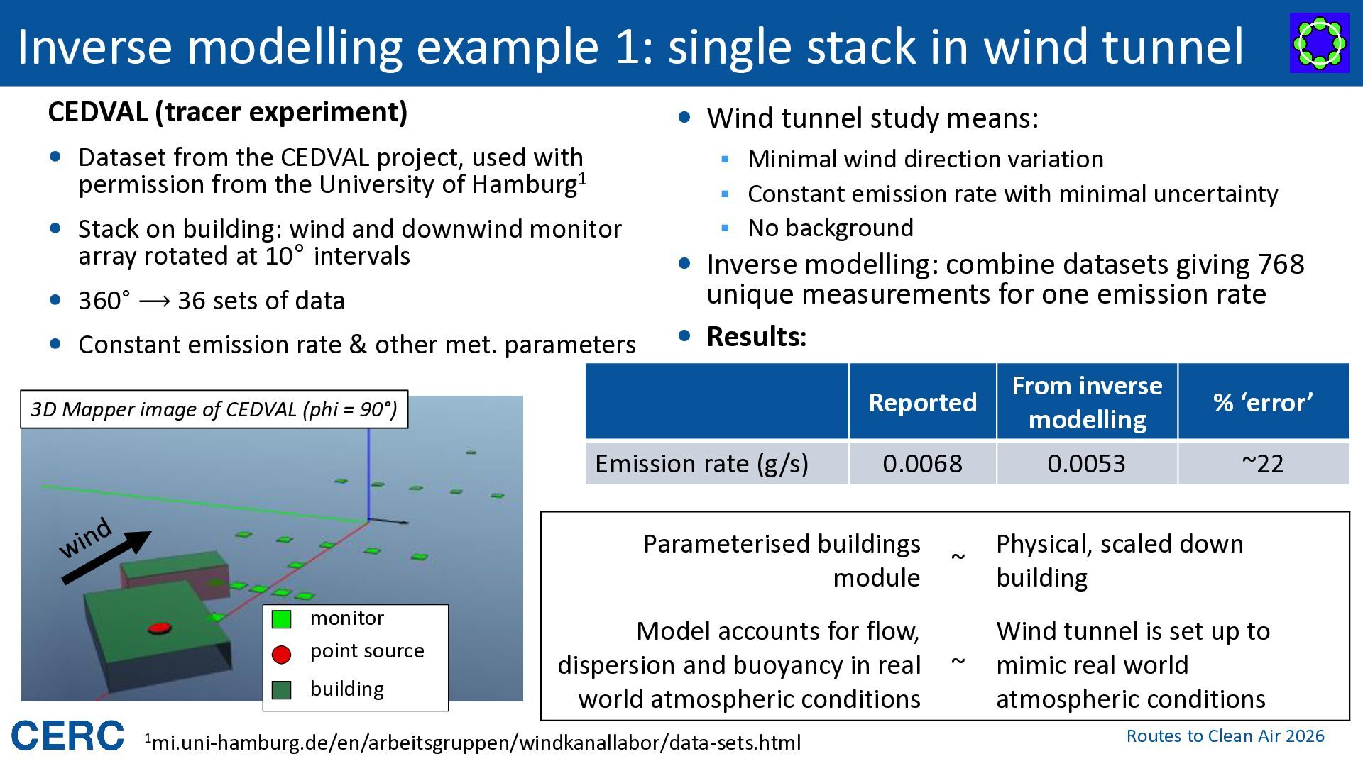
13. Inverse modelling example 1: single stack in wind tunnel CEDVAL (tracer experiment)  Wind tunnel study means:  Dataset from the CEDVAL project, used with ▪ Minimal wind direction variation permission from the University of Hamburg1 ▪ Constant emission rate with minimal uncertainty  Stack on building: wind and downwind monitor array rotated at 10° intervals ▪ No background  Inverse modelling: combine datasets giving 768  360° ⟶ 36 sets of data  Constant emission rate & other met. parameters unique measurements for one emission rate  Results: 3D Mapper image of CEDVAL (phi = 90°) Emission rate (g/s) Reported From inverse modelling % ‘error’ 0.0068 0.0053 ~22 Parameterised buildings module monitor point source building Model accounts for flow, dispersion and buoyancy in real world atmospheric conditions 1mi.uni-hamburg.de/en/arbeitsgruppen/windkanallabor/data-sets.html ~ Physical, scaled down building ~ Wind tunnel is set up to mimic real world atmospheric conditions Routes to Clean Air 2026
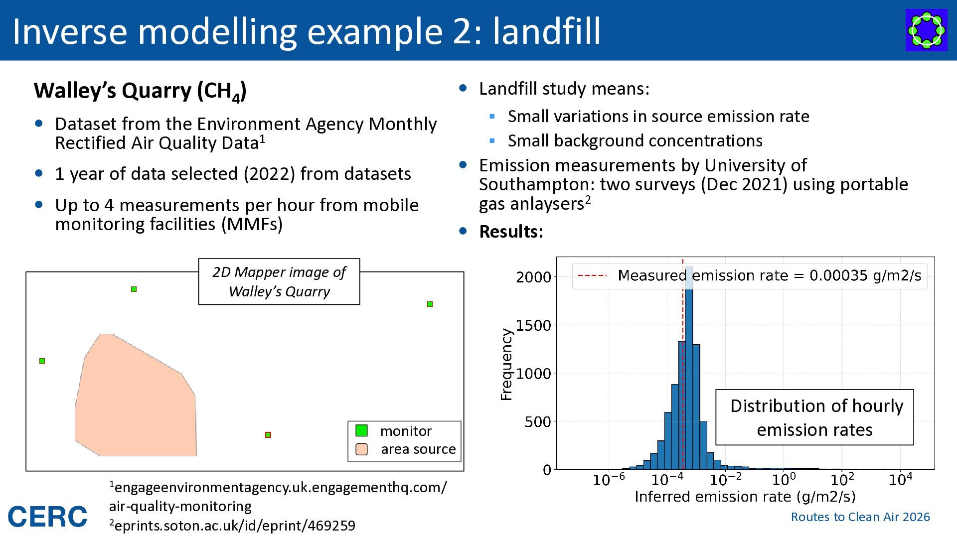
14. Inverse modelling example 2: landfill Walley’s Quarry (CH4)  Dataset from the Environment Agency Monthly Rectified Air Quality Data1  1 year of data selected (2022) from datasets  Up to 4 measurements per hour from mobile monitoring facilities (MMFs)  Landfill study means: ▪ Small variations in source emission rate ▪ Small background concentrations  Emission measurements by University of Southampton: two surveys (Dec 2021) using portable gas anlaysers2  Results: 2D Mapper image of Walley’s Quarry monitor area source Distribution of hourly emission rates 1engageenvironmentagency.uk.engagementhq.com/ air-quality-monitoring 2eprints.soton.ac.uk/id/eprint/469259 Routes to Clean Air 2026
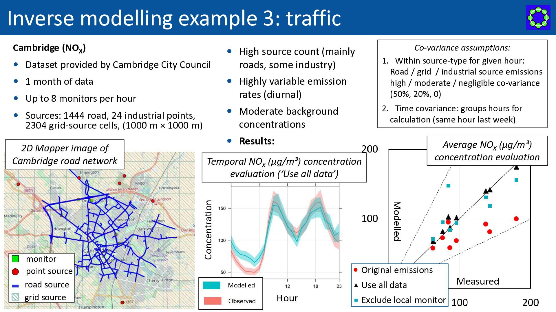
15. Inverse modelling example 3: traffic Cambridge (NOX)  High source count (mainly  Dataset provided by Cambridge City Council  Highly variable emission  1 month of data rates (diurnal)  Up to 8 monitors per hour  Moderate background  Sources: 1444 road, 24 industrial points, concentrations 2304 grid-source cells, (1000 m × 1000 m) Average NOX (µg/m³) concentration evaluation Temporal NOX (µg/m³) concentration evaluation (‘Use all data’) Modelled monitor point source road source grid source 2. Time covariance: groups hours for calculation (same hour last week)  Results: Concentration 2D Mapper image of Cambridge road network roads, some industry) Co-variance assumptions: 1. Within source-type for given hour: Road / grid / industrial source emissions high / moderate / negligible co-variance (50%, 20%, 0) Measured Modelled Hour Routes to Clean Air 2026
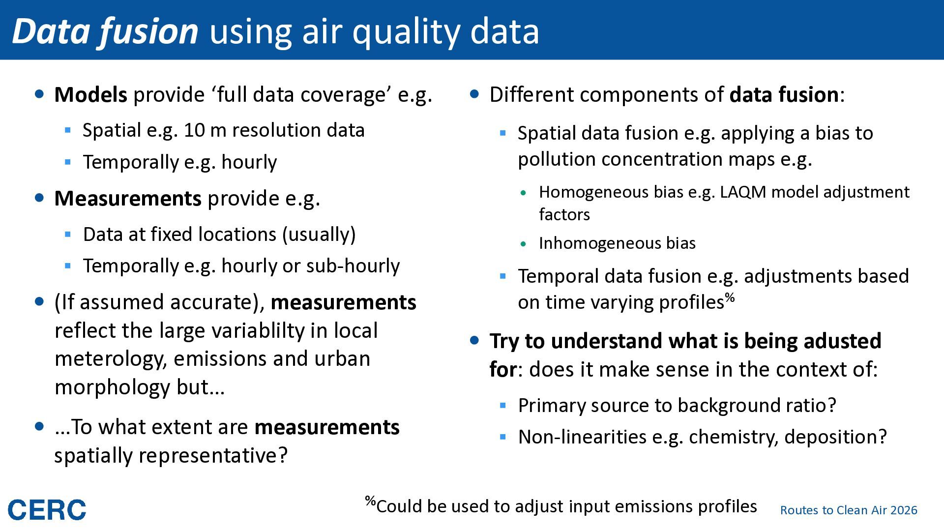
16. Data fusion using air quality data  Models provide ‘full data coverage’ e.g. ▪ Spatial e.g. 10 m resolution data ▪ Spatial data fusion e.g. applying a bias to pollution concentration maps e.g. ▪ Temporally e.g. hourly  Measurements provide e.g. ▪ Data at fixed locations (usually) ▪ Temporally e.g. hourly or sub-hourly  (If assumed accurate), measurements reflect the large variablilty in local meterology, emissions and urban morphology but…  …To what extent are measurements spatially representative?  Different components of data fusion:  Homogeneous bias e.g. LAQM model adjustment factors  Inhomogeneous bias ▪ Temporal data fusion e.g. adjustments based on time varying profiles%  Try to understand what is being adusted for: does it make sense in the context of: ▪ Primary source to background ratio? ▪ Non-linearities e.g. chemistry, deposition? %Could be used to adjust input emissions profiles Routes to Clean Air 2026
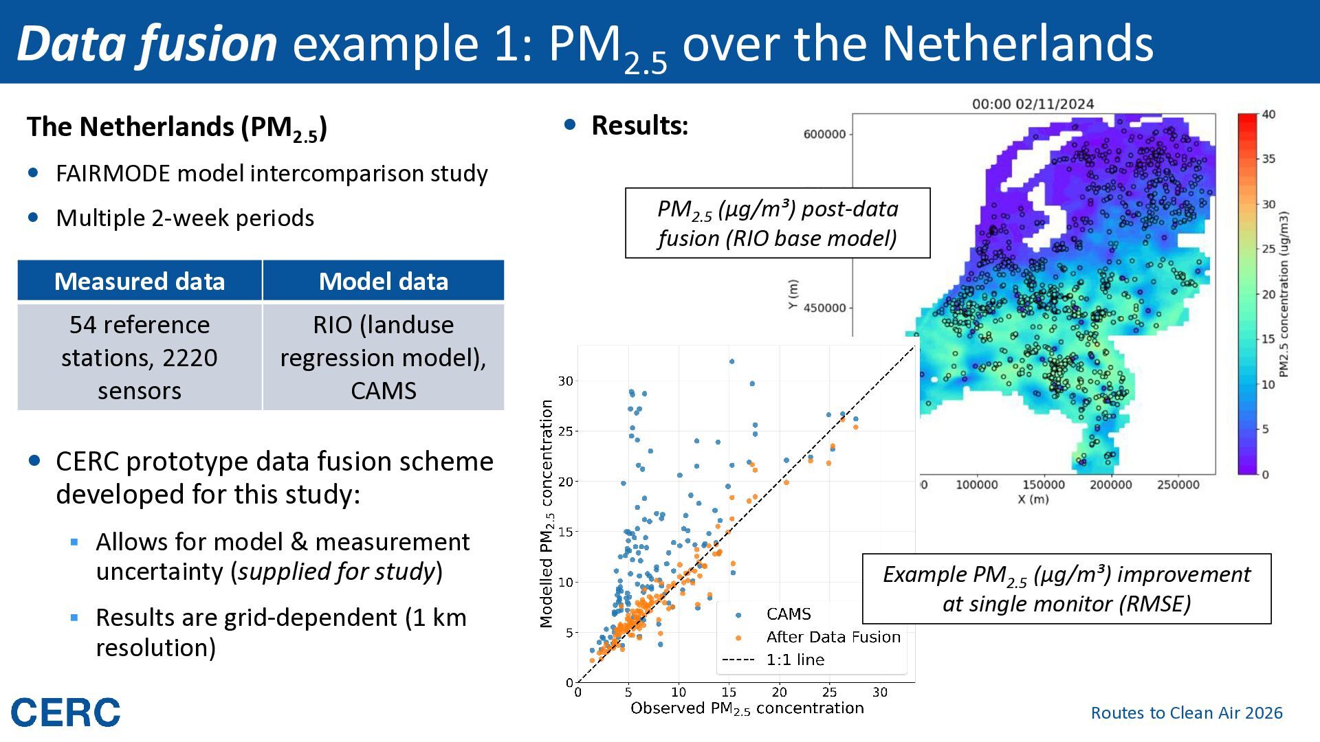
17. Data fusion example 1: PM2.5 over the Netherlands The Netherlands (PM2.5)  Results:  FAIRMODE model intercomparison study PM2.5 (µg/m³) post-data fusion (RIO base model)  Multiple 2-week periods Measured data Model data 54 reference stations, 2220 sensors RIO (landuse regression model), CAMS  CERC prototype data fusion scheme developed for this study: ▪ Allows for model & measurement uncertainty (supplied for study) ▪ Results are grid-dependent (1 km Example PM2.5 (µg/m³) improvement at single monitor (RMSE) resolution) Routes to Clean Air 2026
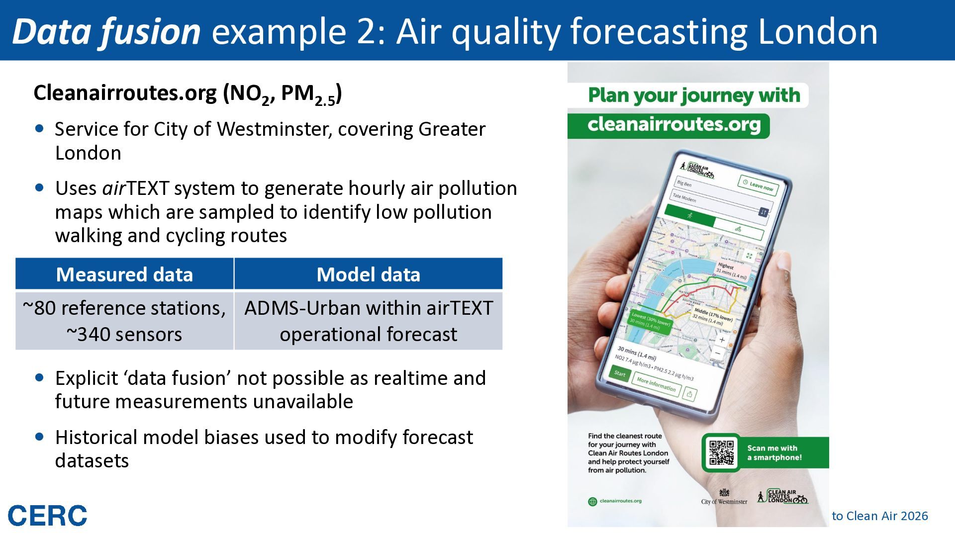
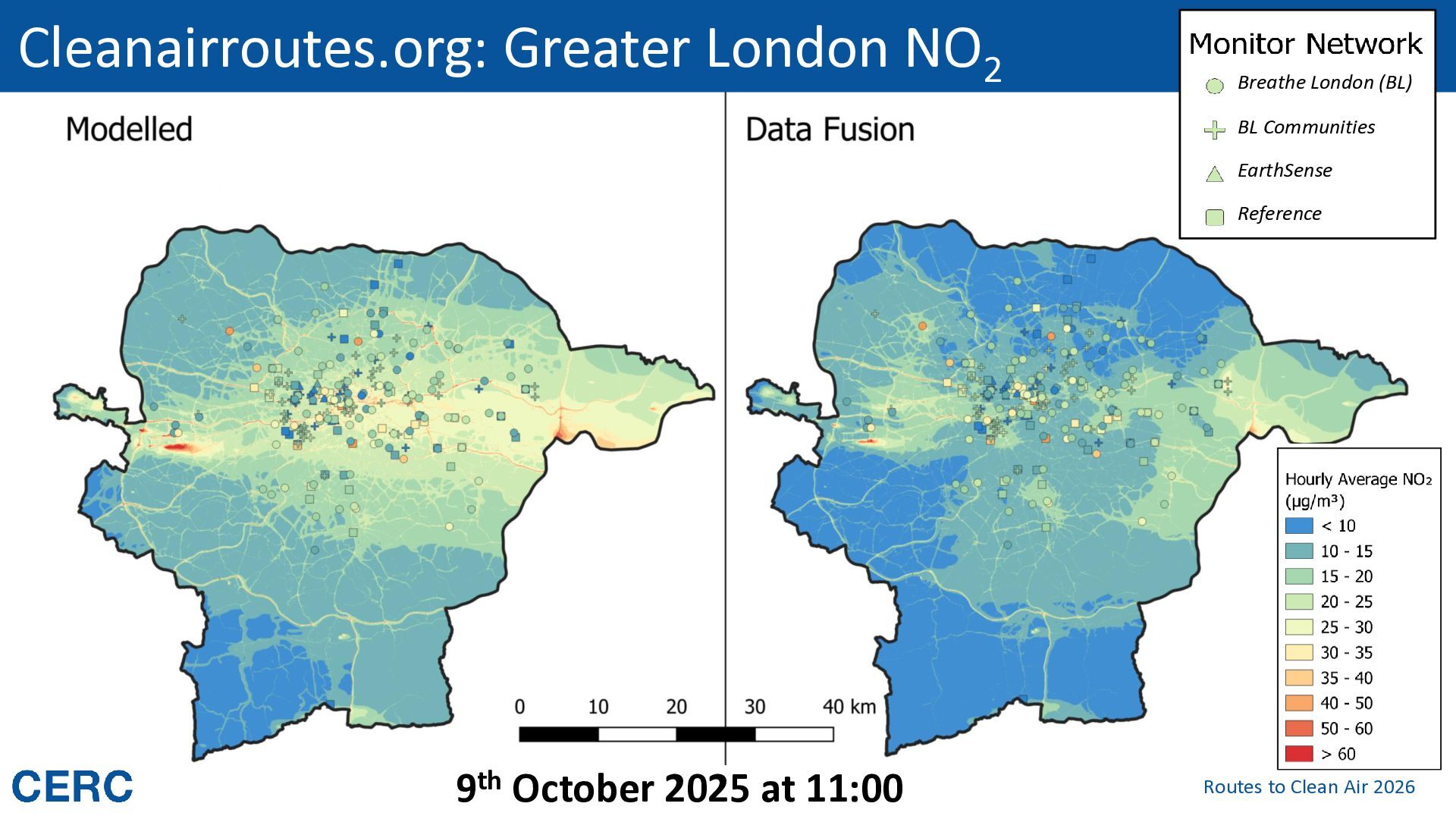
18. Data fusion example 2: Air quality forecasting London Cleanairroutes.org (NO2, PM2.5)  Service for City of Westminster, covering Greater London  Uses airTEXT system to generate hourly air pollution maps which are sampled to identify low pollution walking and cycling routes Measured data Model data ~80 reference stations, ADMS-Urban within airTEXT ~340 sensors operational forecast  Explicit ‘data fusion’ not possible as realtime and future measurements unavailable  Historical model biases used to modify forecast datasets Routes to Clean Air 2026
19. Cleanairroutes.org: Greater London NO2 Breathe London (BL) BL Communities EarthSense Reference 9th October 2025 at 11:00 Routes to Clean Air 2026
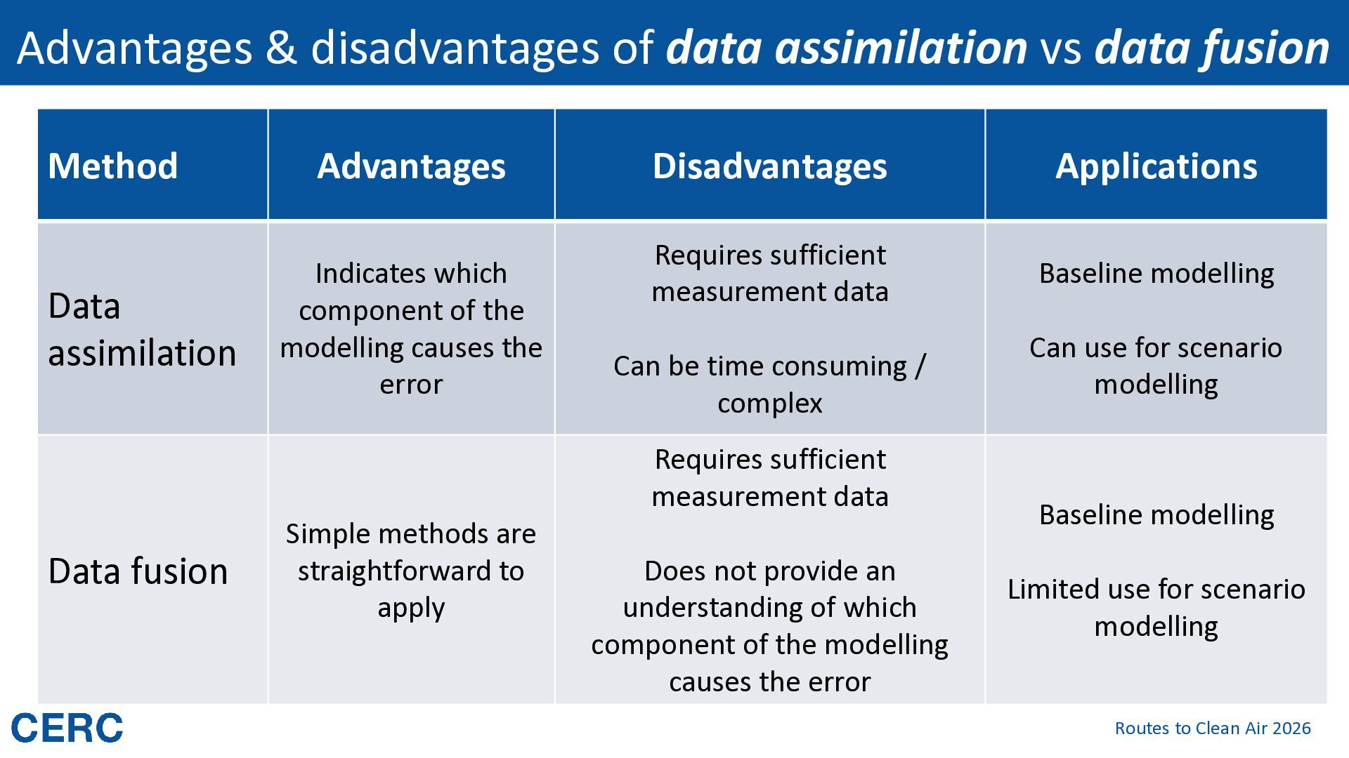
20. Advantages & disadvantages of data assimilation vs data fusion Method Data assimilation Advantages Indicates which component of the modelling causes the error Disadvantages Applications Requires sufficient measurement data Baseline modelling Can be time consuming / complex Requires sufficient measurement data Data fusion Simple methods are straightforward to apply Does not provide an understanding of which component of the modelling causes the error Can use for scenario modelling Baseline modelling Limited use for scenario modelling Routes to Clean Air 2026
21. Inverse modelling Emissions factors Data assimilation: improving model inputs Source activity data Questions? Jenny.Stocker@cerc.co.uk Met & background data Routes to Clean Air 2026