RTCA Dr Nosha Assareh - The UK Compliance Air Quality Modelling System: Methods, components, and policy applications

Transcript

1. UK compliance modelling Components and policy applications Nosha Assareh Environmental Research Group, Imperial College London Routes to Clean Air (RTCA) 2026 n.assareh@imperial.ac.uk
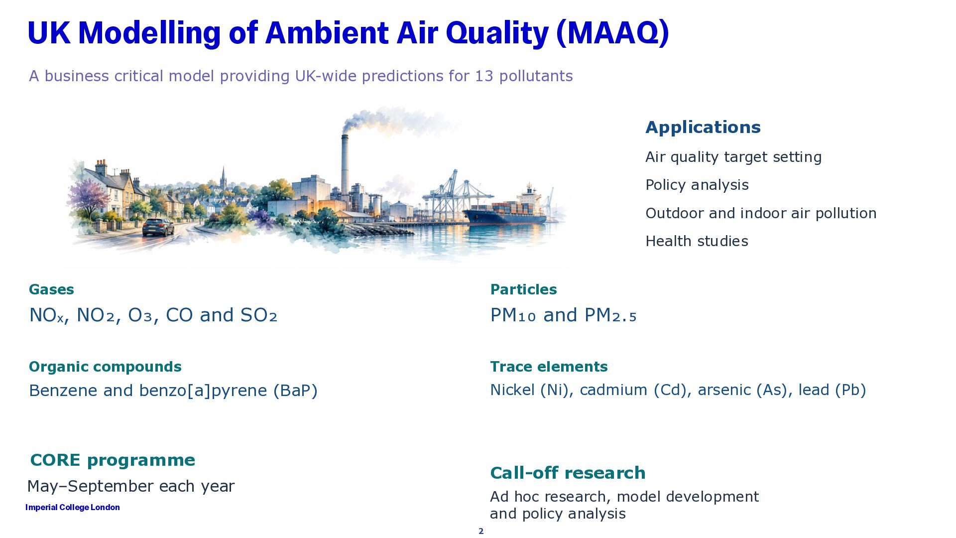
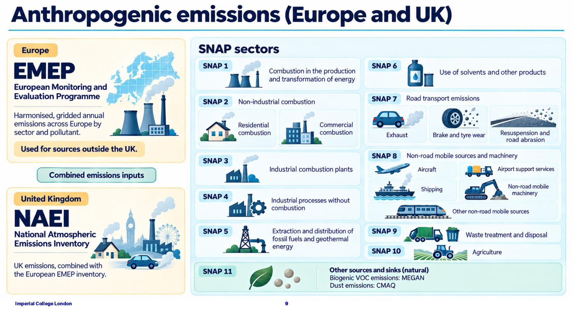
2. UK Modelling of Ambient Air Quality (MAAQ) A business critical model providing UK-wide predictions for 13 pollutants Applications Air quality target setting Policy analysis Outdoor and indoor air pollution Health studies Gases Particles NOₓ, NO₂, O₃, CO and SO₂ PM₁₀ and PM₂.₅ Organic compounds Trace elements Benzene and benzo[a]pyrene (BaP) Nickel (Ni), cadmium (Cd), arsenic (As), lead (Pb) CORE programme Call-off research May–September each year Ad hoc research, model development and policy analysis Imperial College London 2
3. MAAQ flow diagram Imperial College London 3
4. Modelling domains and outputs Air pollution outputs Imperial College London Road-by-road estimates • 1 km national maps • 20–100 m industrial results 6
5. WRF meteorology Imperial College London 5
6. CMAQ chemistry and transport Imperial College London 6 10/26/2026
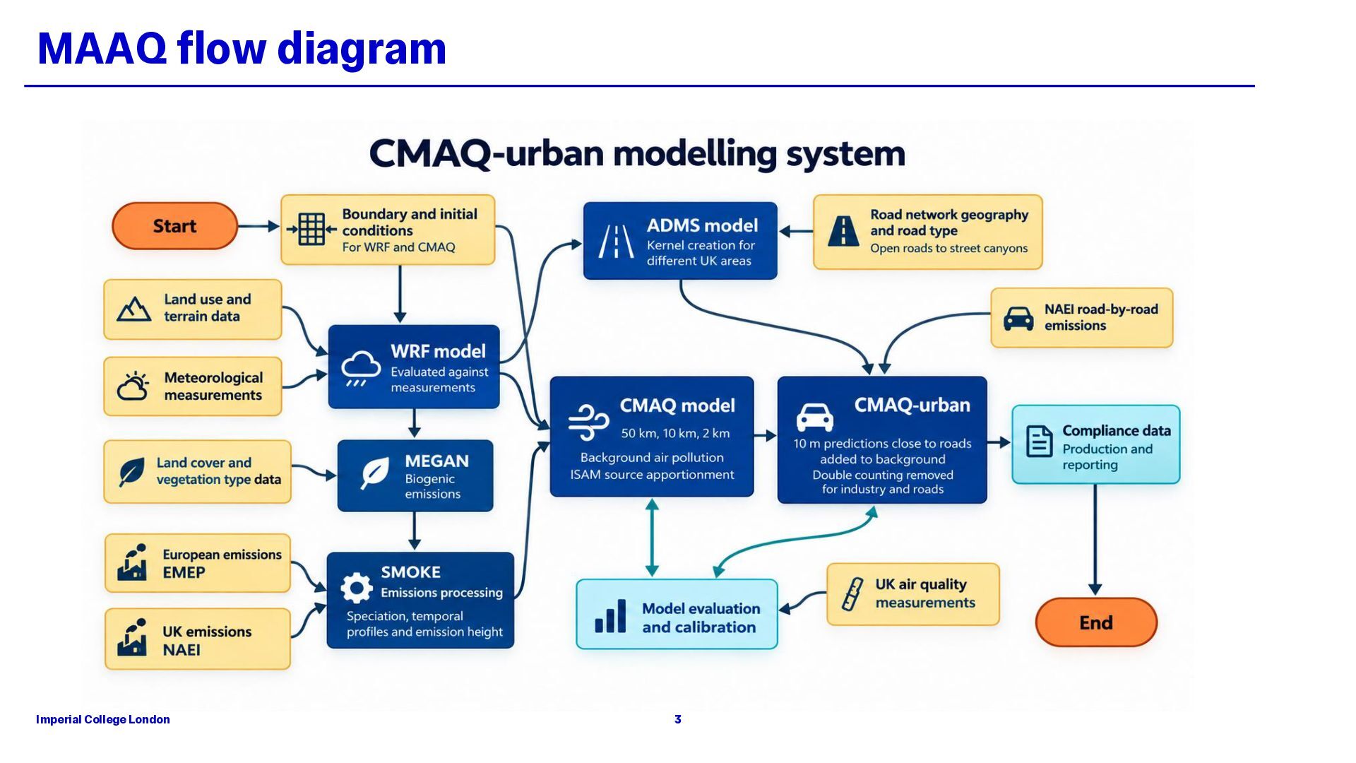
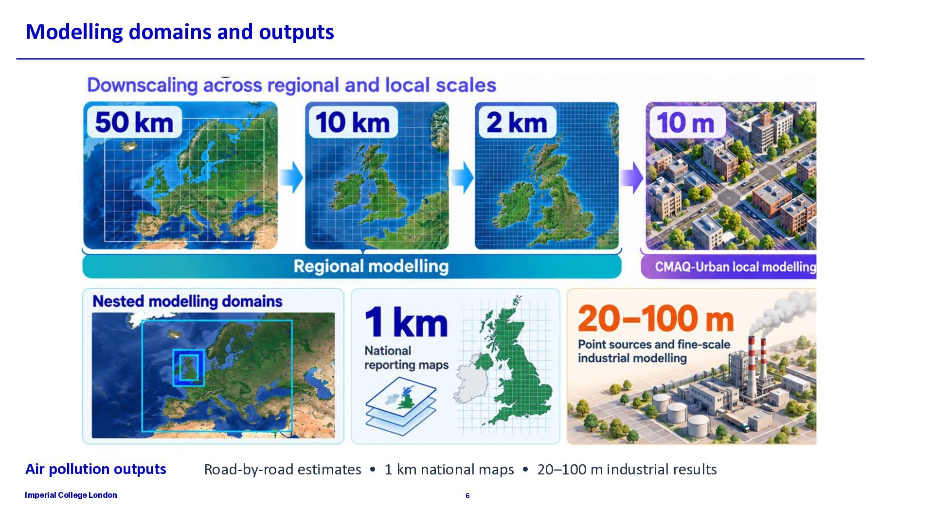
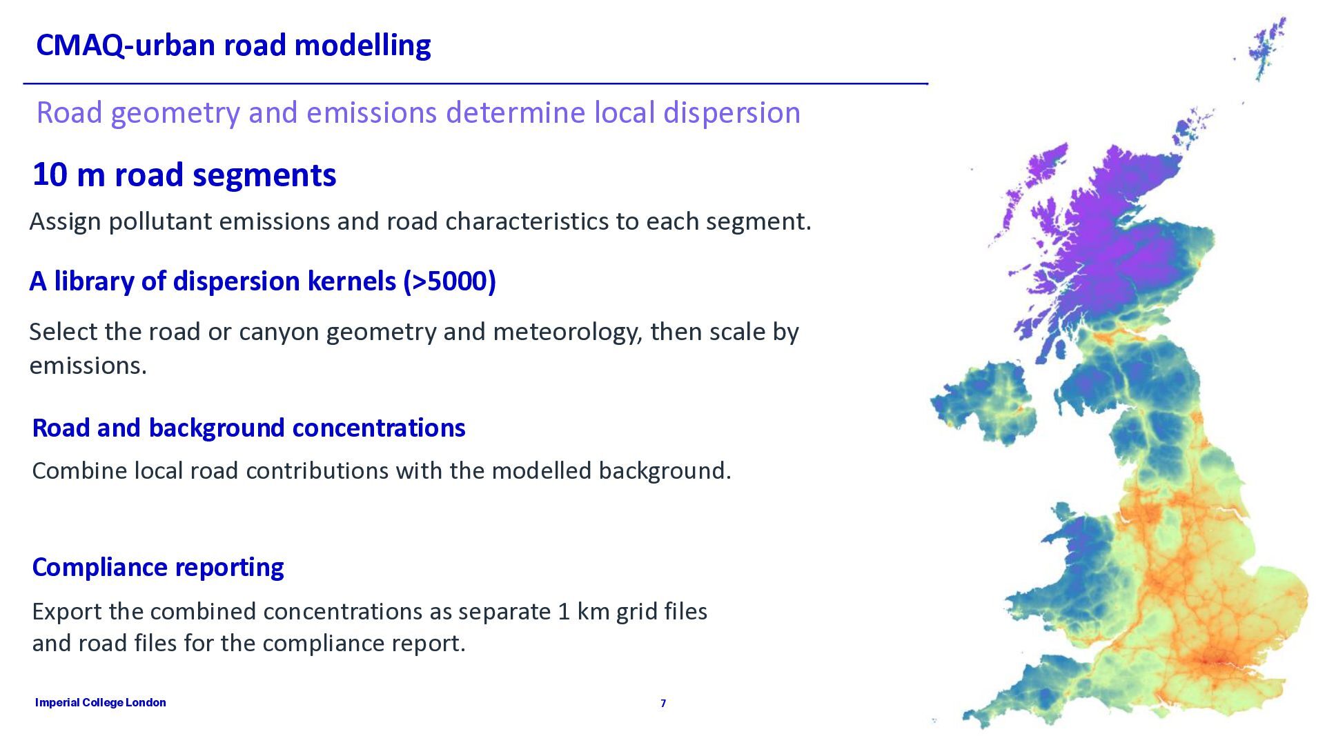
7. CMAQ-urban road modelling Road geometry and emissions determine local dispersion 10 m road segments Assign pollutant emissions and road characteristics to each segment. A library of dispersion kernels (>5000) Select the road or canyon geometry and meteorology, then scale by emissions. Road and background concentrations Combine local road contributions with the modelled background. Compliance reporting Export the combined concentrations as separate 1 km grid files and road files for the compliance report. Imperial College London 7
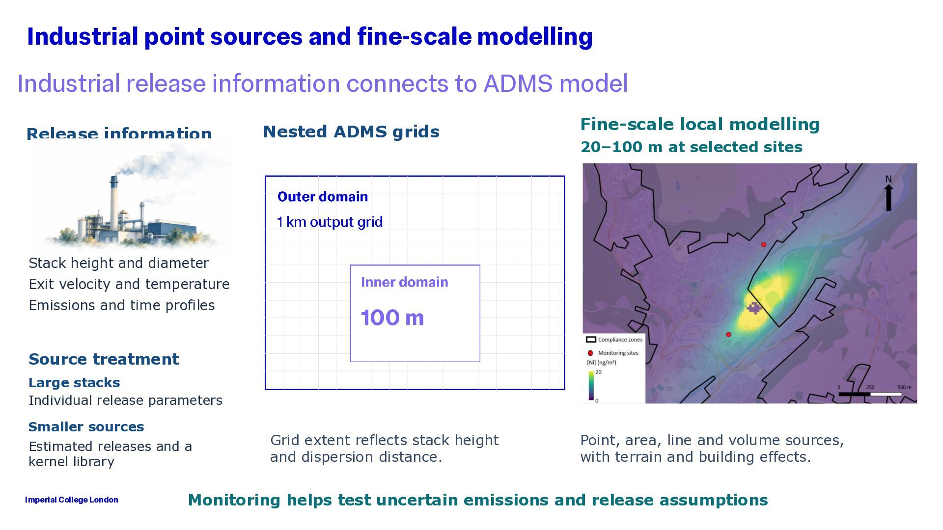
8. Industrial point sources and fine-scale modelling Industrial release information connects to ADMS model Release information Nested ADMS grids Fine-scale local modelling 20–100 m at selected sites Stack height and diameter Exit velocity and temperature Emissions and time profiles Source treatment Large stacks Individual release parameters Smaller sources Estimated releases and a kernel library Imperial College London Grid extent reflects stack height and dispersion distance. Point, area, line and volume sources, with terrain and building effects. Monitoring helps test uncertain emissions and release assumptions
9. Emission inventories Imperial College London 9
10. MEGAN biogenic emissions Imperial College London 10 10/26/2026
11. SMOKE emissions processing Imperial College London 11 10/26/2026
12. ISAM source tagging Imperial College London 12
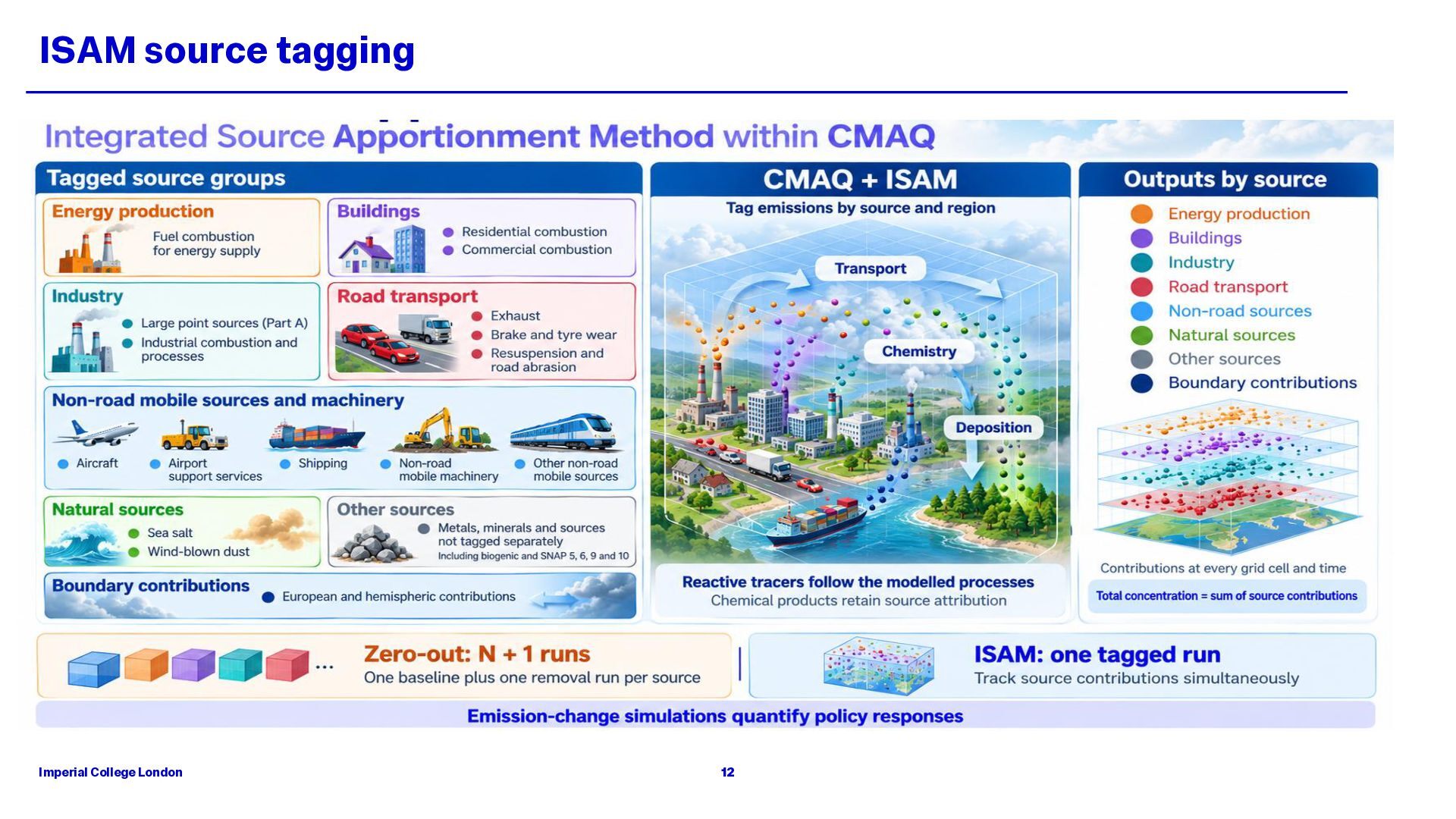
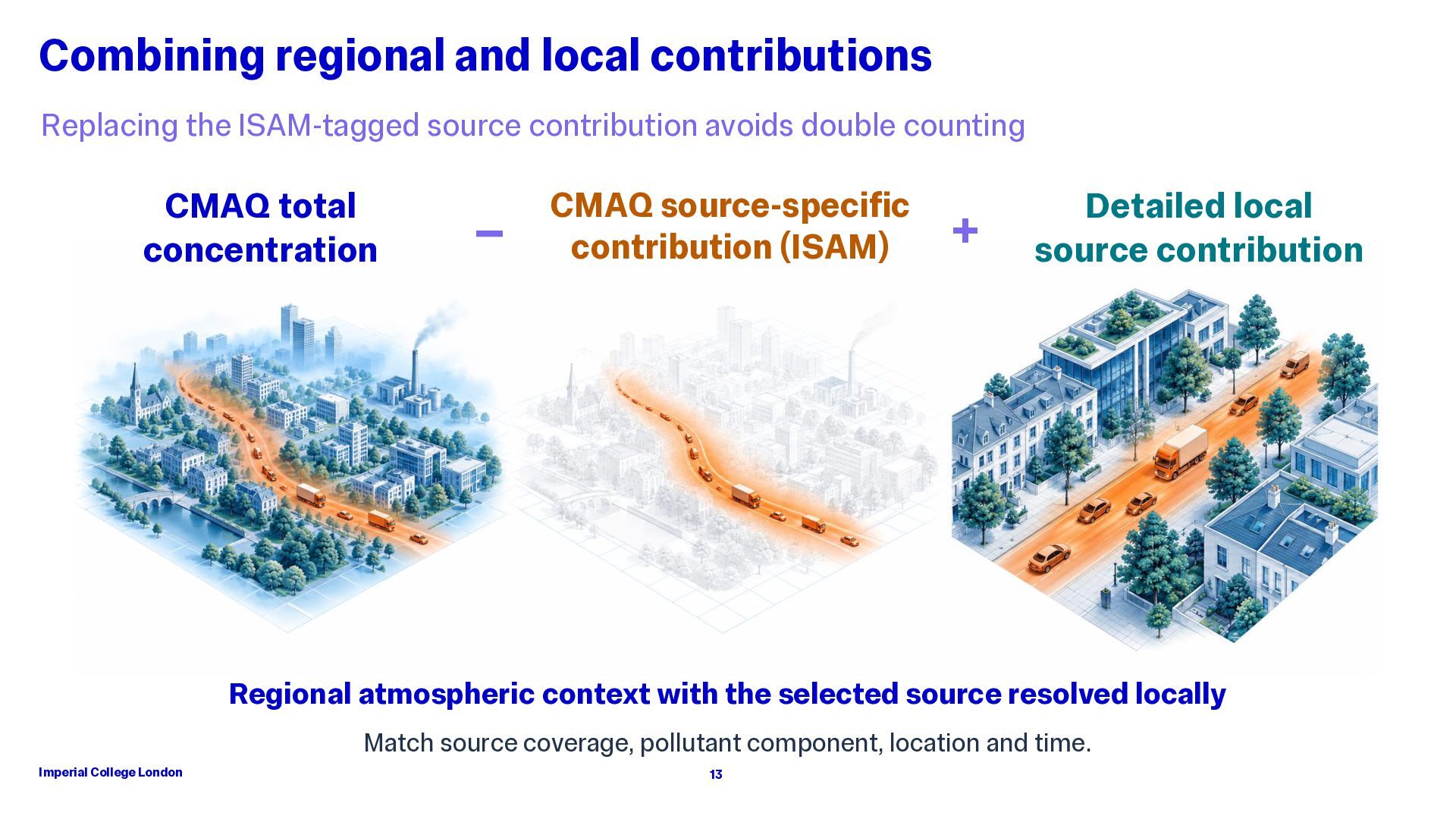
13. Combining regional and local contributions Replacing the ISAM-tagged source contribution avoids double counting CMAQ total concentration − CMAQ source-specific contribution (ISAM) + Detailed local source contribution Regional atmospheric context with the selected source resolved locally Match source coverage, pollutant component, location and time. Imperial College London 13
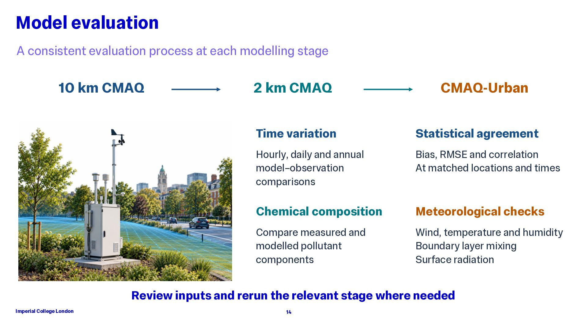
14. Model evaluation A consistent evaluation process at each modelling stage 10 km CMAQ 2 km CMAQ CMAQ-Urban Time variation Statistical agreement Hourly, daily and annual model–observation comparisons Bias, RMSE and correlation At matched locations and times Chemical composition Meteorological checks Compare measured and modelled pollutant components Wind, temperature and humidity Boundary layer mixing Surface radiation Review inputs and rerun the relevant stage where needed Imperial College London 14
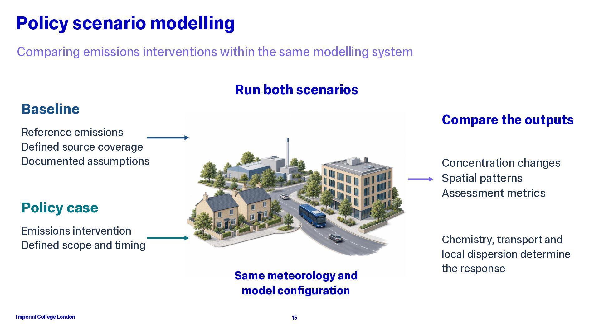
15. Policy scenario modelling Comparing emissions interventions within the same modelling system Run both scenarios Baseline Compare the outputs Reference emissions Defined source coverage Documented assumptions Concentration changes Spatial patterns Assessment metrics Policy case Emissions intervention Defined scope and timing Same meteorology and model configuration Imperial College London 15 Chemistry, transport and local dispersion determine the response
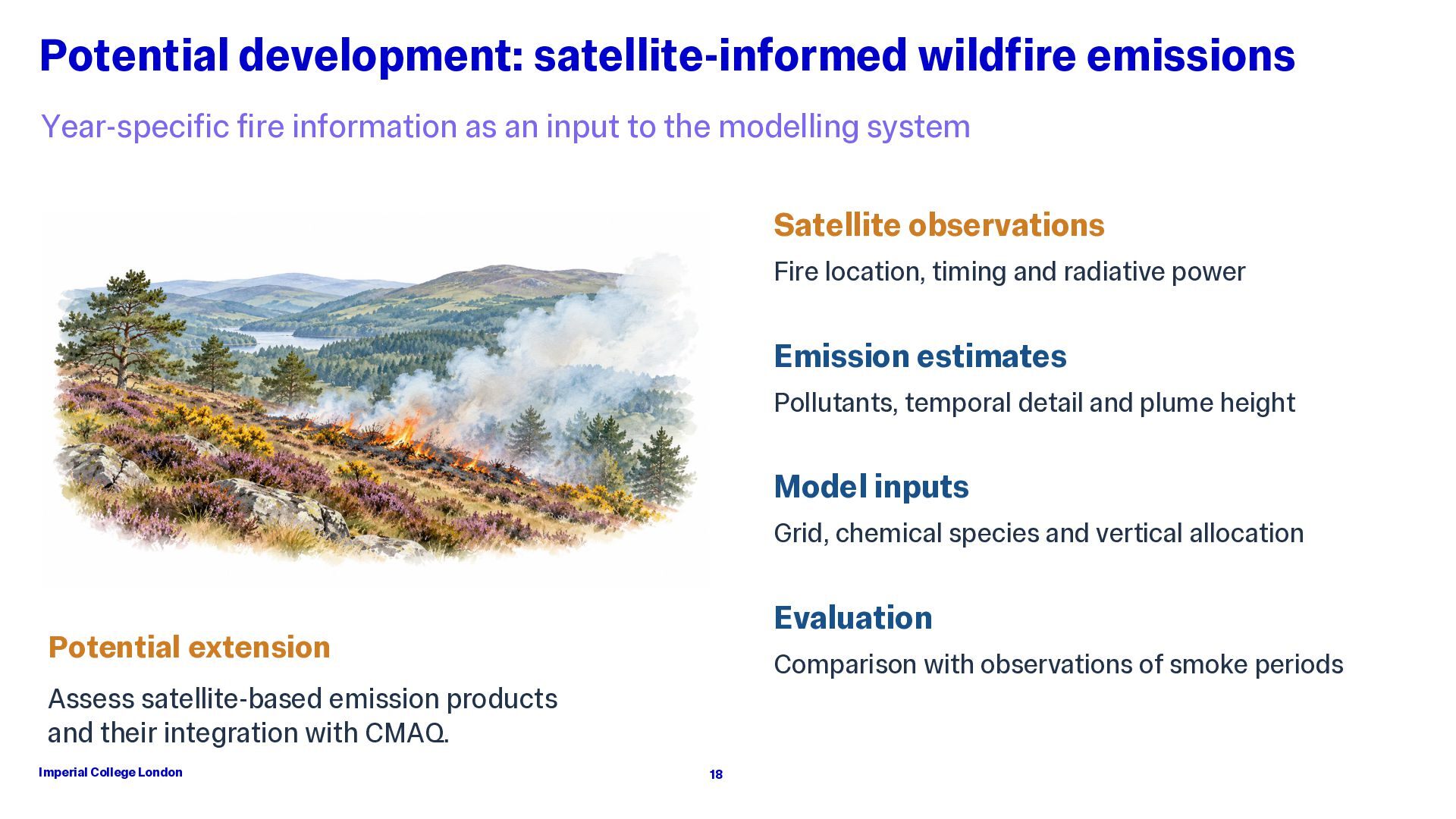
16. Potential development: satellite-informed wildfire emissions Year-specific fire information as an input to the modelling system Satellite observations Fire location, timing and radiative power Emission estimates Pollutants, temporal detail and plume height Model inputs Grid, chemical species and vertical allocation Evaluation Potential extension Comparison with observations of smoke periods Assess satellite-based emission products and their integration with CMAQ. Imperial College London 18
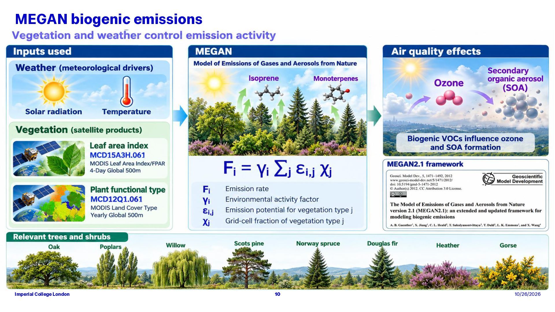
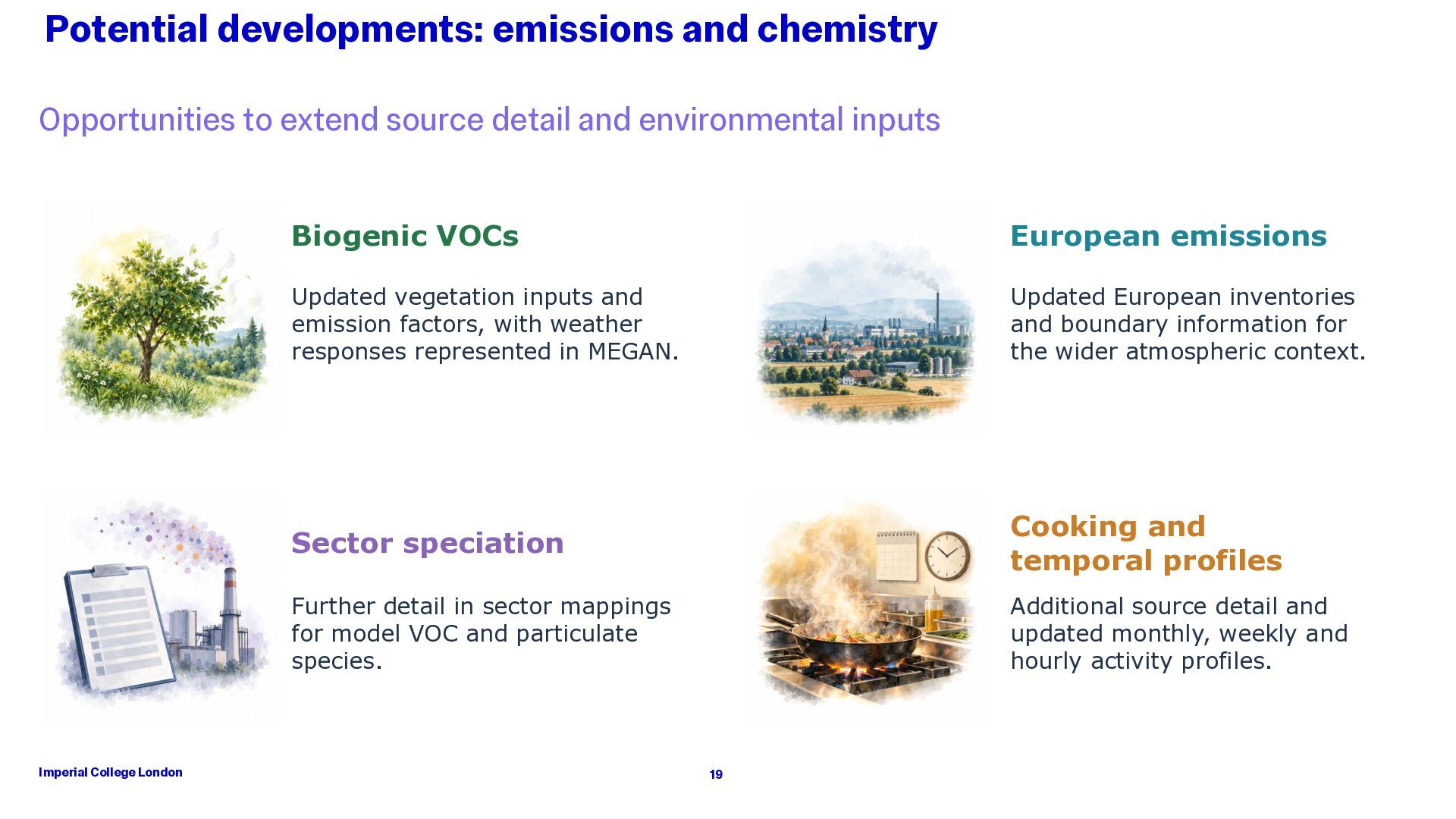
17. Potential developments: emissions and chemistry Opportunities to extend source detail and environmental inputs Imperial College London Biogenic VOCs European emissions Updated vegetation inputs and emission factors, with weather responses represented in MEGAN. Updated European inventories and boundary information for the wider atmospheric context. Sector speciation Cooking and temporal profiles Further detail in sector mappings for model VOC and particulate species. Additional source detail and updated monthly, weekly and hourly activity profiles. 19
18. Potential developments: Roadside Model Diagnosis Imperial College London Edit this text via Insert > Header and Footer 18
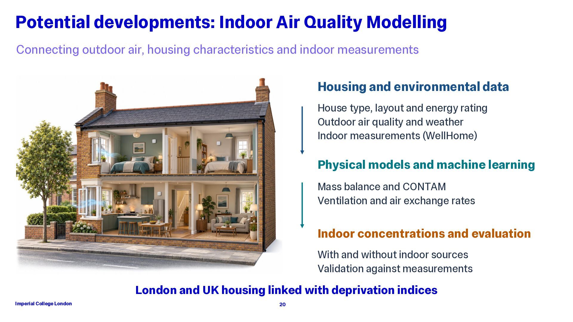
19. Potential developments: Indoor Air Quality Modelling Connecting outdoor air, housing characteristics and indoor measurements Housing and environmental data House type, layout and energy rating Outdoor air quality and weather Indoor measurements (WellHome) Physical models and machine learning Mass balance and CONTAM Ventilation and air exchange rates Indoor concentrations and evaluation With and without indoor sources Validation against measurements London and UK housing linked with deprivation indices Imperial College London 20
20. Questions and acknowledgements UK compliance modelling, components and policy applications Thank you Nosha Assareh n.assareh@imperial.ac.uk Sean Beevers, Andrew Beddows, Gregor Stewart, David Dajnak, Yuanlin Wang and Gargi Sengupta Imperial College London 20