Surfaces Can be represented by huge number of points (polygons or triangles) + arbitrary shapes possible – large memory requirements – changes cause much work – corners - scaling Can be represented by two sets of orthogonal curves – only for some shape categories + marginal memory requirements + changes are rather simple + definition arbitrarily exact 3
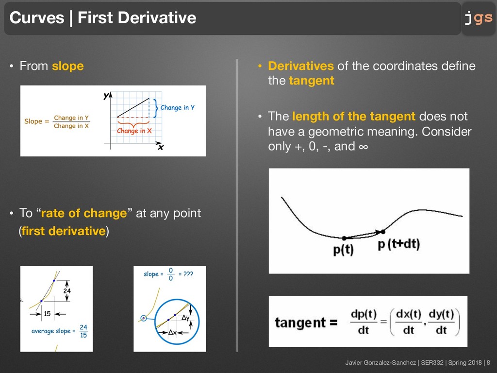
• Derivatives of the coordinates define the tangent • The length of the tangent does not have a geometric meaning. Consider only +, 0, -, and ∞ • From slope • To “rate of change” at any point (first derivative) Curves | First Derivative
• Derivatives of the coordinates define the tangent • The length of the tangent does not have a geometric meaning. Consider only +, 0, -, and ∞ • From slope • To “rate of change” at any point (first derivative) Curves | First Derivative
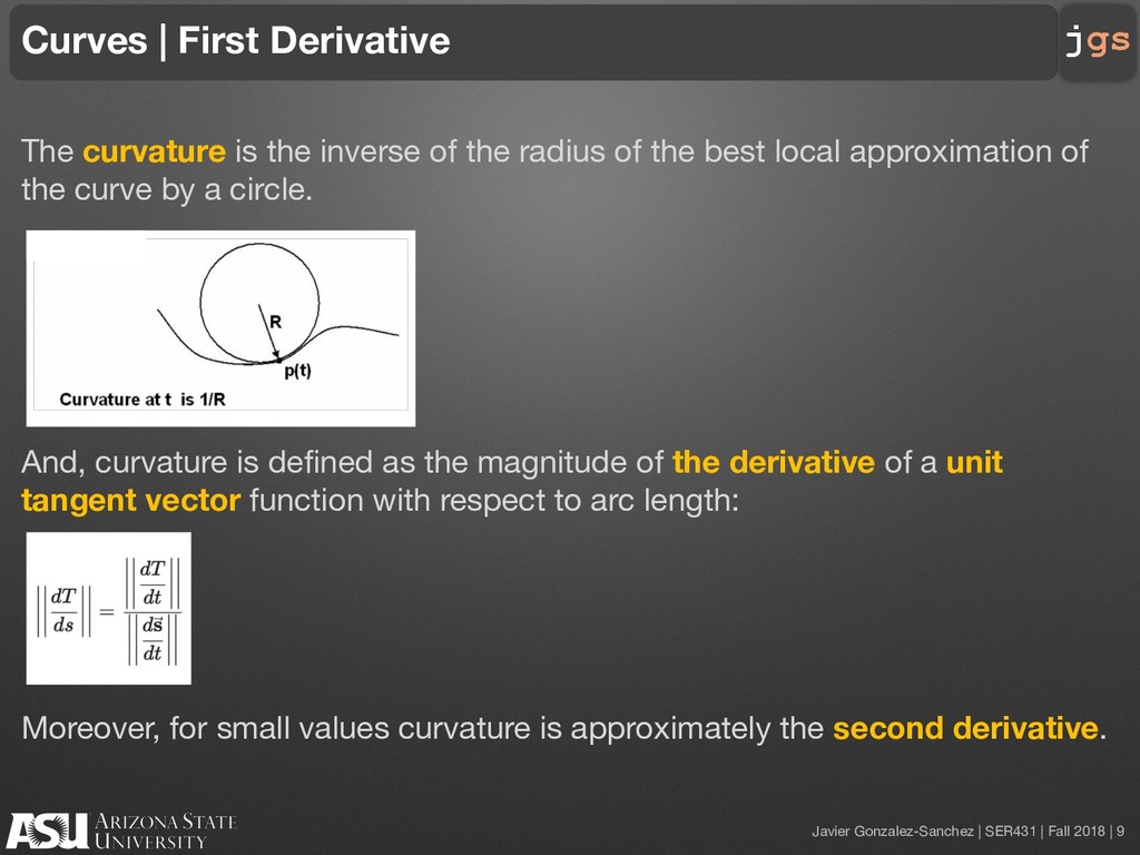
Curves | First Derivative The curvature is the inverse of the radius of the best local approximation of the curve by a circle. And, curvature is defined as the magnitude of the derivative of a unit tangent vector function with respect to arc length: Moreover, for small values curvature is approximately the second derivative.
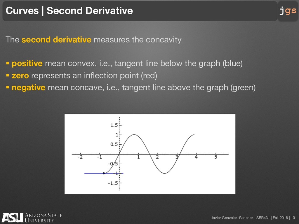
Curves | Second Derivative The second derivative measures the concavity § positive mean convex, i.e., tangent line below the graph (blue) § zero represents an inflection point (red) § negative mean concave, i.e., tangent line above the graph (green)
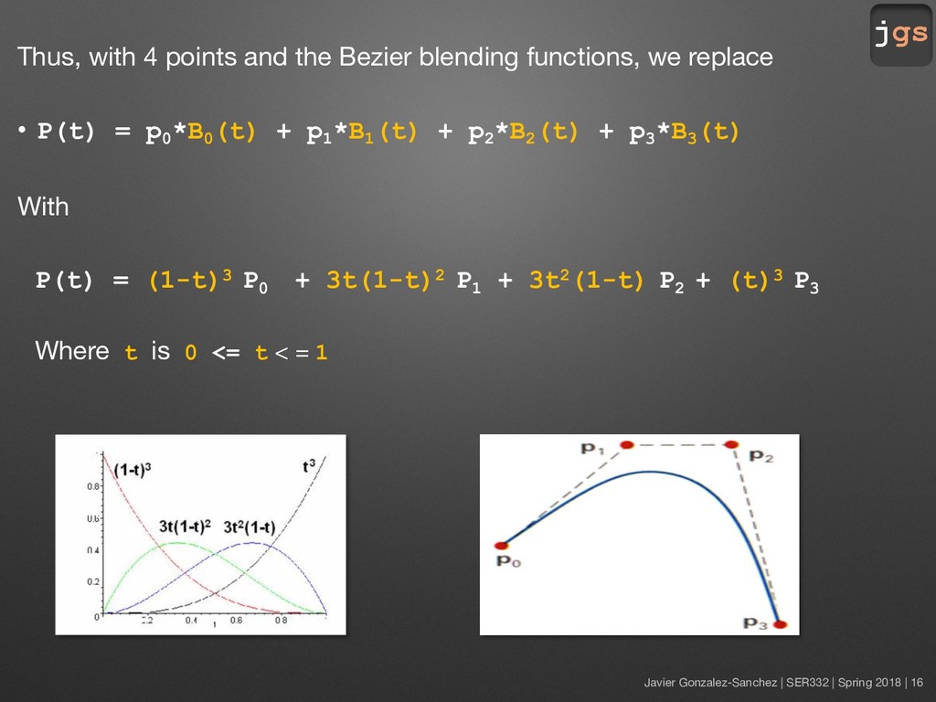
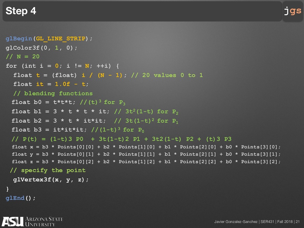
Curves and Splines § A curve can be a concatenation of splines. § Control points determine the shape of the spline curve. § For each point specify a blending function which determines how the control point influence the shape of the curve for values of parameter t. § Therefore, a curve spline is specified as P(t) = p0 *B0 (t) + p1 *B1 (t) + p2 *B2 (t) + p3 *B3 (t) + ... § This is axis independent, i.e., it does not change when the coordinate system is rotated. 12
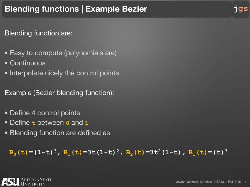
Blending functions | Example Bezier Blending function are: § Easy to compute (polynomials are) § Continuous § Interpolate nicely the control points Example (Bezier blending function): § Define 4 control points § Define t between 0 and 1 § Blending function are defined as B0 (t)=(1-t)3, B1 (t)=3t(1-t)2, B2 (t)=3t2(1-t), B1 (t)=(t)3
Blending functions | Example Bezier Blending function are: § Easy to compute (polynomials are) § Continuous § Interpolate nicely the control points Example (Bezier blending function): § Define 4 control points § Define t between 0 and 1 § Blending function are defined as B0 (t)=(1-t)3, B1 (t)=3t(1-t)2, B2 (t)=3t2(1-t), B1 (t)=(t)3
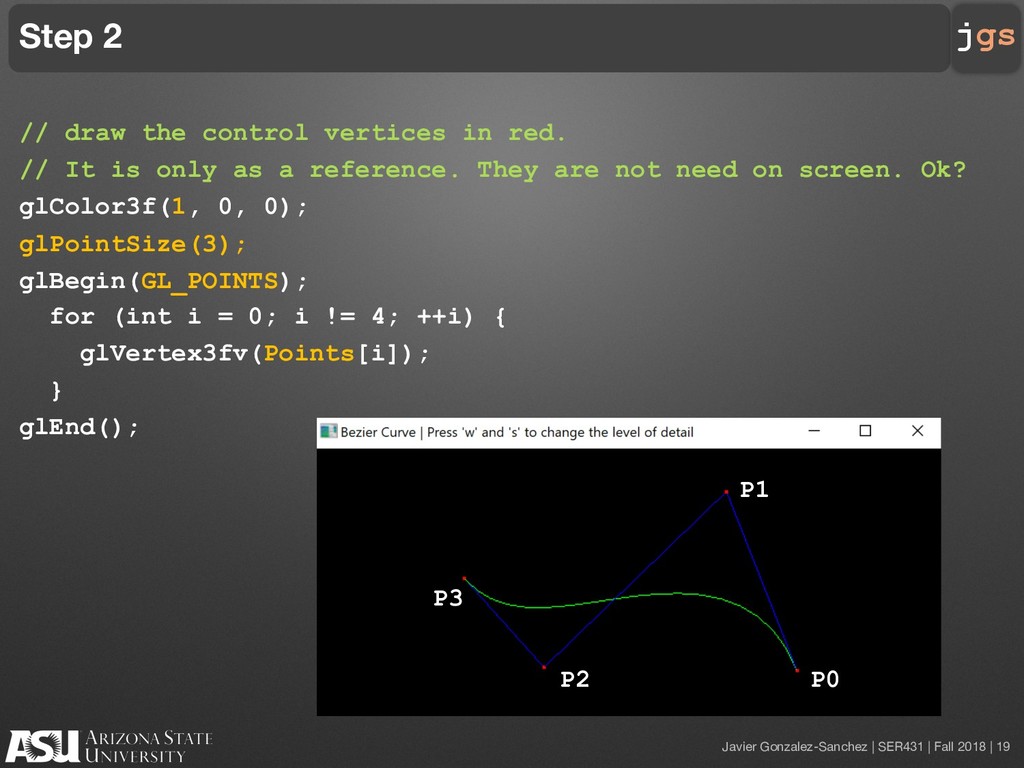
Step 2 // draw the control vertices in red. // It is only as a reference. They are not need on screen. Ok? glColor3f(1, 0, 0); glPointSize(3); glBegin(GL_POINTS); for (int i = 0; i != 4; ++i) { glVertex3fv(Points[i]); } glEnd(); P3 P0 P1 P2
Step 3 // control graph in blue glColor3f(0, 0, 1); glBegin(GL_LINE_STRIP); for (int i = 0; i != 4; ++i) { glVertex3fv(Points[i]); } glEnd(); P3 P0 P1 P2
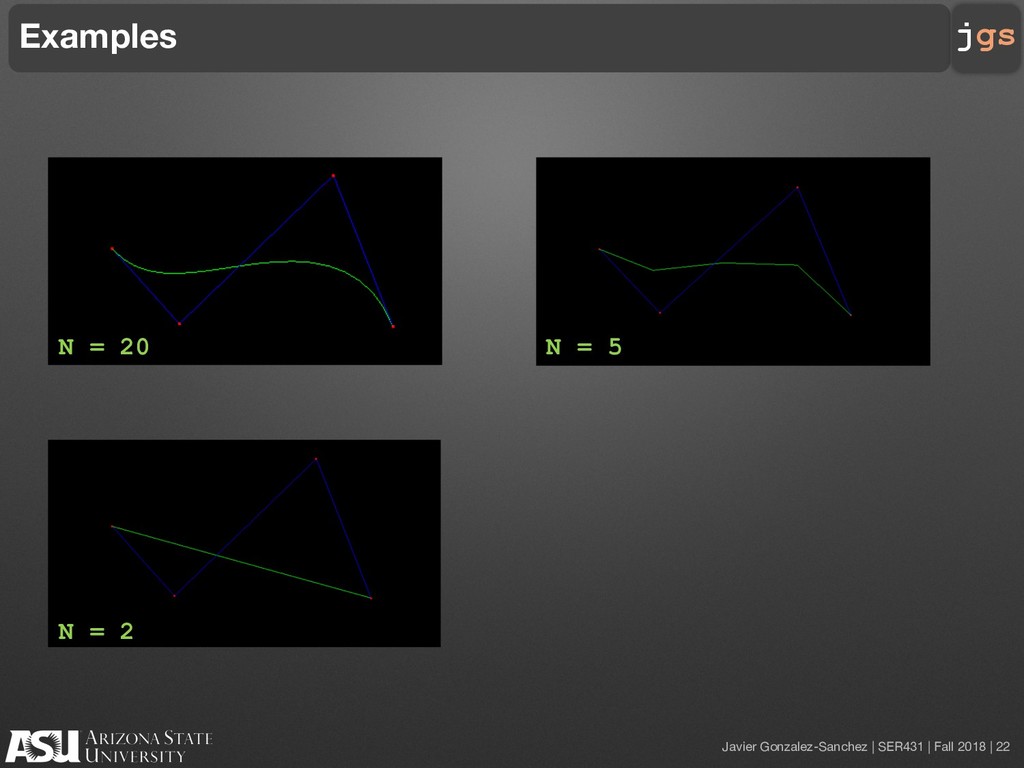
§ Review the source code posted on GitHub Test yourselves: § Change the coordinates of the control points; for instance, play with diverse combinations of positive and negative x and y. § Draw a second Bezier spline adjacent to the first one § Draw a second Bezier spline parallel to the first one Homework
![jgs SER431 Advanced Graphics Javier Gonzalez-Sanchez [email protected] Fall 2018 Disclaimer.](https://files.speakerdeck.com/presentations/5aefc695a08244b4b44360724449b403/slide_23.jpg)