Modeling Motor Learning

Transcript

1. 1 MODELING MOTOR LEARNING USING HETEROSKEDASTIC FUNCTIONAL PRINCIPAL COMPONENTS ANALYSIS JEFF GOLDSMITH, PHD DEPARTMENT OF BIOSTATISTICS
2. 2 Acknowledgements • Daniel Backenroth, Michelle D. Harran, Juan C. Cortes, John W. Krakauer, Tomoko Kitago • Funded by R21EB018917, R01NS097423, and R01HL123407
3. 3 Interest is in motor learning • People get better at motor tasks through practice • Mean change can be minimal for simple tasks • Variance change can be relatively large
4. 4 Experiment set-up
5. 5 Kinematic data • • • • • • • • −20 −10 0 10 20 −20 −10 0 10 20 X Y −20 −10 0 10 20 0 10 20 PX(t) 20 20
6. 6 Dataset • 26 right-handed subjects • 24 motions to each target with each hand • Target direction was semi-randomized • Data are [PX ij (t), PY ij (t)]
7. 7 Kinematic data • • • • • • • • −20 −10 0 10 20 −20 −10 0 10 20 X Y −20 −10 0 10 20 0 10 20 30 40 50 t PX(t) −20 −10 0 10 20 0 10 20 30 40 50 t PY(t) • • • • • • • • −20 −10 0 10 20 −20 −10 0 10 20 X Y −20 −10 0 10 20 0 10 20 30 40 50 t PX(t) −20 −10 0 10 20 0 10 20 30 40 50 t PY(t)
8. 8 Traditional FPCA Pij(t) = µij(t) + ij(t) = µij(t) + K X k=1 ⇠ijk k(t) + ✏ij(t) Scores are uncorrelated random variables with and . ⇠ijk E(⇠ijk) = 0 var(⇠ijk) = k
9. 9 Problem • Distribution of the scores determines the variability curves • Motion variance can depend on baseline motor control or training ⇠ijk Constant variance is wrong for our data.
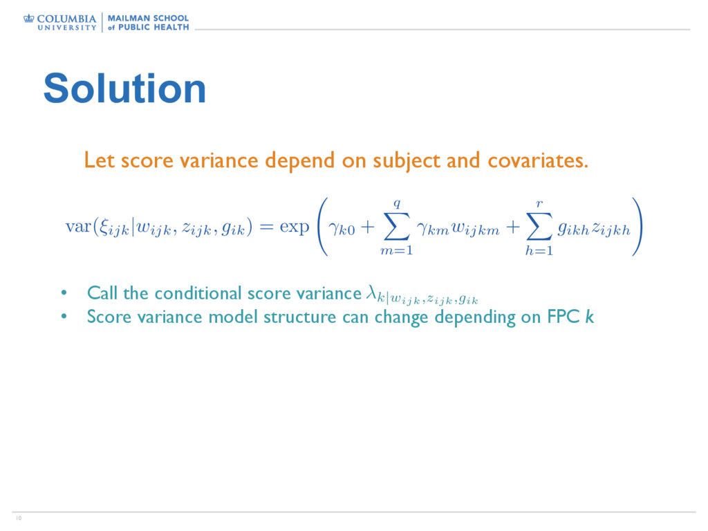
10. 10 Solution • Call the conditional score variance • Score variance model structure can change depending on FPC k Let score variance depend on subject and covariates. var( ⇠ijk |wijk, zijk, gik) = exp k0 + q X m=1 kmwijkm + r X h=1 gikhzijkh ! k|wijk,zijk,gik
11. 11 Implications I Conditional covariance cov[ ij( s ) , ij( t ) |wijk, zijk, gik] = K X k=1 k|wijk,zijk,gik k( s ) k( t )
12. 12 Implications II Marginal covariance cov[ ij( s ) , ij( t )] = K X k=1 E ⇥ k|wijk,zijk,gik ⇤ k( s ) k( t )
13. 13 Assumptions I • Scores still need to have mean zero • We model the mean using function-on-scalar regression: µij( t ) = 0( t ) + p X l=1 xijl l( t ) + bi( t )
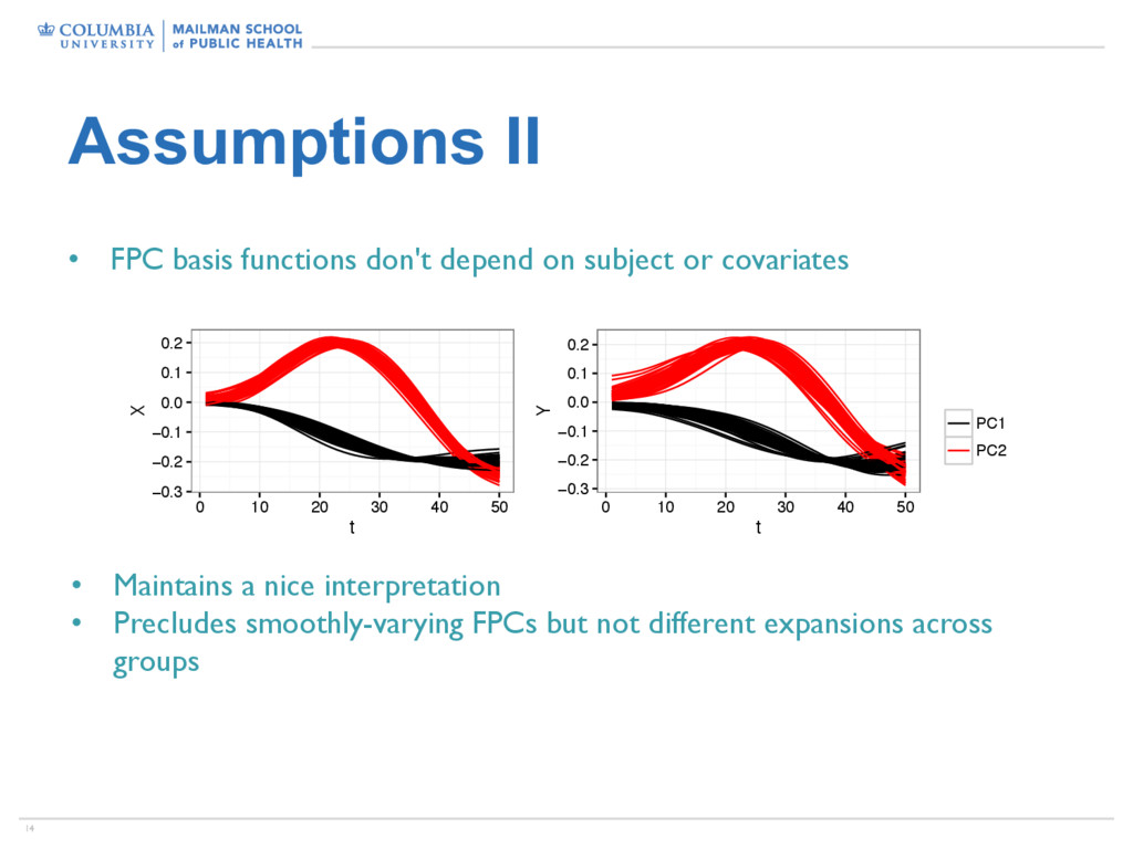
14. 14 Assumptions II • FPC basis functions don't depend on subject or covariates • Maintains a nice interpretation • Precludes smoothly-varying FPCs but not different expansions across groups −0.3 −0.2 −0.1 0.0 0.1 0.2 0 10 20 30 40 50 t X −0.3 −0.2 −0.1 0.0 0.1 0.2 0 10 20 30 40 50 t Y PC1 PC2
15. 15 Alternatives • Build a model for the scores directly (Chiou et al 2003) • Implies some covariate dependence in the variance, but mostly focuses on the mean • Allow complete covariance to be covariate dependent (Jiang and Wang 2010) • Non-constant FPCs are harder to interpret • Difficult to posit complex models
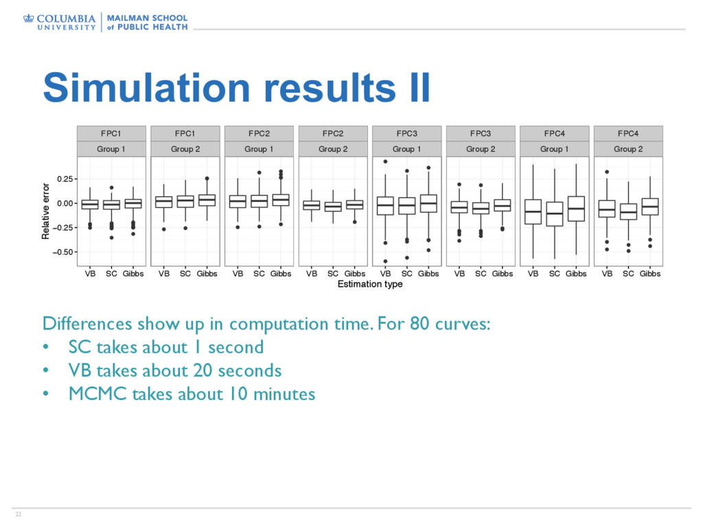
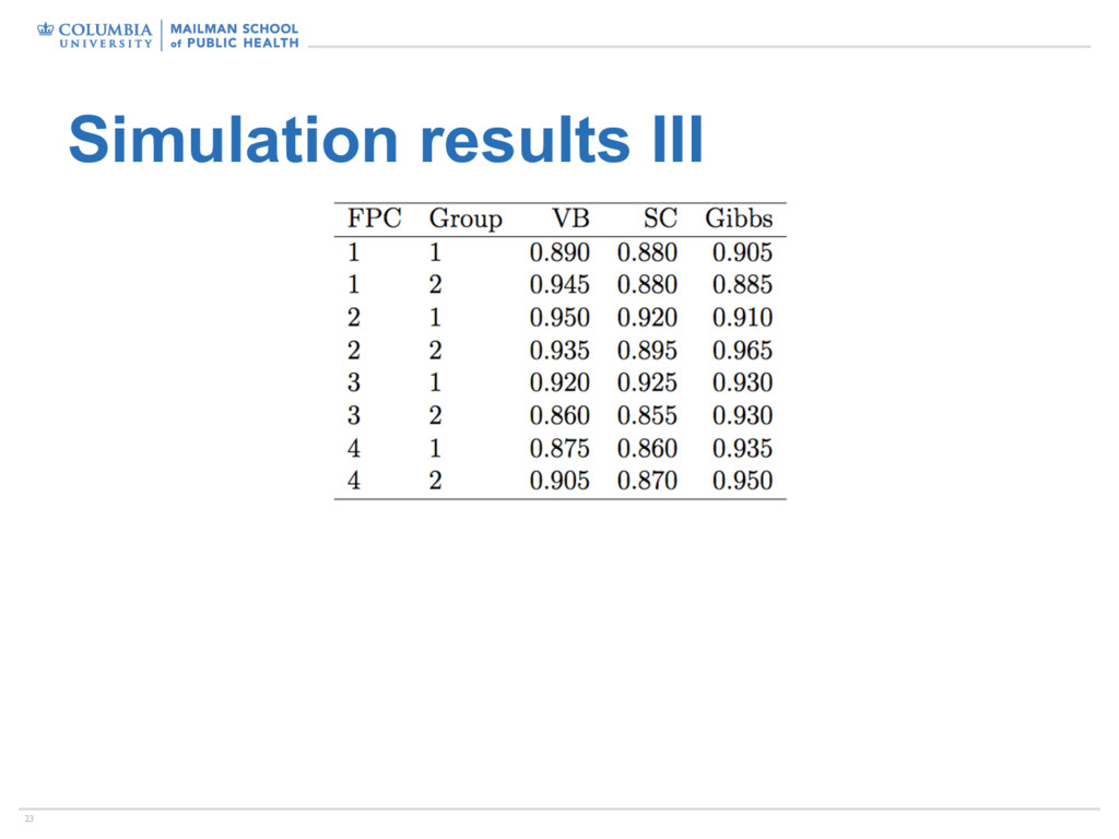
16. 16 Estimation Several possible approaches: • Smooth covariance decomposition + score estimation + score variance model • Probabilistic / Bayesian FPCA • Variational Bayes • MCMC Advantages and disadvantages for each We tried each and compared in simulations
17. 17 Bayesian model
18. 18 Rotations • Model specification didn't constrain orthogonality • Needed for scores to be interpretable across iterations • Quick work-around: SVD step in the sampler / VB algorithm
19. 19 Cross sectional simulation design I • and are and • and are and • • • pi(t) = 0 + 4 X k=1 ⇠ik k(t) + ✏i(t) t 2 [0, 2⇡] I 2 {20, 40, 80, 160, 320} 2 = 0.25 1(t) 2(t) 3(t) 4(t) sin(t) cos( t ) sin(2t) cos(2 t )
20. 20 Cross sectional simulation design II Score Variances FPC 1 FPC 2 FPC 3 FPC 4 Group 1 36 12 6 4 Group 1I 18 24 12 6 pi(t) = 0 + 4 X k=1 ⇠ik k(t) + ✏i(t) Single binary covariate:
21. 21 Simulation results I FPC1 FPC2 FPC3 FPC4 −0.2 −0.1 0.0 0.1 0.2 0 10 20 30 40 50 0 10 20 30 40 50 0 10 20 30 40 50 0 10 20 30 40 50 t • • • • • • • • • • • • • • • • • • • • • • • • • • • • • • • • • • • • • • • • • • • • • • • • • • • • • • • • • • • • • • • • • • • • • • • • • • • • • • • • • • • • • • • • • • • • • • • • • • • • • • • • • • • • • • • • • • • • • • • • • • • • • • • • • • • • • • • • • • • • • • • • • • • • • • • • • • • • • • • • • • • • • • • • • • • • • • • • • • • • • • • • • • • • • • • • • • • • • • • • • • • • • • • • • • • • • • • • • • • • • • • • • • • • • • • • • FPC1 FPC2 FPC3 FPC4 0.0 0.5 1.0 1.5 2.0 20 40 80 160 320 20 40 80 160 320 20 40 80 160 320 20 40 80 160 320 Number of curves ISE • • • • • • • • • • • • • • • • • • • • • • • • • • • • • • • • • • • • • • • • • • • • • • • • • • • • • • • • • • • • • • • • • • • • • • • • • • • • • • • • • • • • • • • • • • • • • • • • • • • • • • • • • • • FPC1 Group 1 FPC1 Group 2 FPC2 Group 1 FPC2 Group 2 FPC3 Group 1 FPC3 Group 2 FPC4 Group 1 FPC4 Group 2 −2 −1 0 20 40 80 160320 20 40 80 160320 20 40 80 160320 20 40 80 160320 20 40 80 160320 20 40 80 160320 20 40 80 160320 20 40 80 160320 Number of curves Relative error
22. 22 Simulation results II • • • • • • • • • • • • • • • • • • • • • • • • • • • • • • • • • • • • • • • • • • • • • • • • • • • • • • • • • • • • • • • • • • • FPC1 Group 1 FPC1 Group 2 FPC2 Group 1 FPC2 Group 2 FPC3 Group 1 FPC3 Group 2 FPC4 Group 1 FPC4 Group 2 −0.50 −0.25 0.00 0.25 VB SC Gibbs VB SC Gibbs VB SC Gibbs VB SC Gibbs VB SC Gibbs VB SC Gibbs VB SC Gibbs VB SC Gibbs Estimation type Relative error Differences show up in computation time. For 80 curves: • SC takes about 1 second • VB takes about 20 seconds • MCMC takes about 10 minutes
23. 23 Simulation results III
24. 24 Other simulations • Vary ME variance • Vary dimension of spline basis • Vary truncation lag • Examine multilevel structures
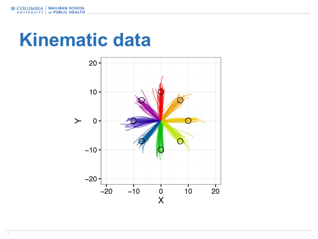
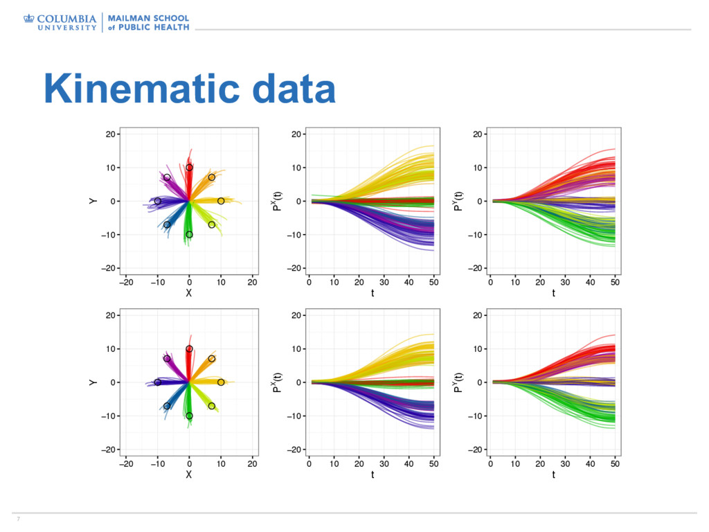
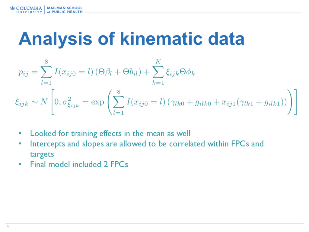
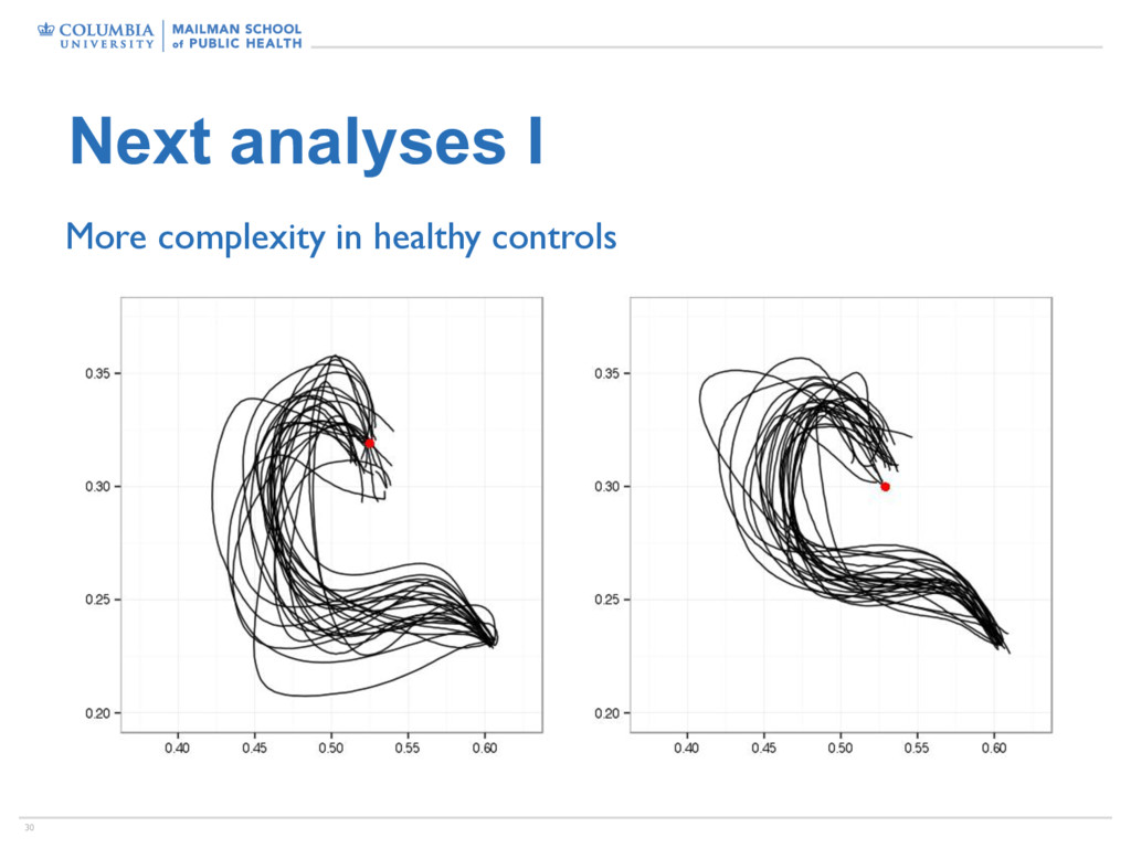
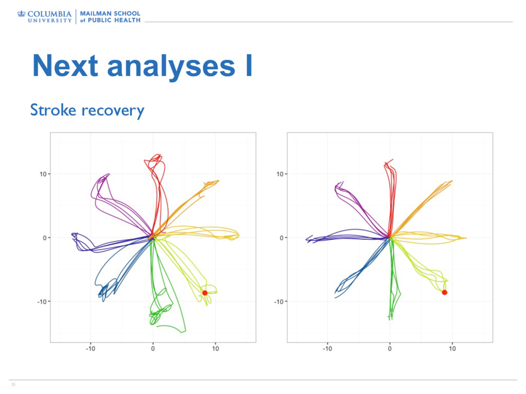
25. 25 Analysis of kinematic data Covariate of interest is repetition number • Allow separate effects for each target • Include subject-specific random intercepts and slopes for each target Prior to analysis, curves are rotated to lie on the positive X axis • Variation in X direction relates to extent • Variation in Y direction relates to direction
26. 26 Analysis of kinematic data • Looked for training effects in the mean as well • Intercepts and slopes are allowed to be correlated within FPCs and targets • Final model included 2 FPCs pij = 8 X l=1 I(xij0 = l) (⇥ l + ⇥bil) + K X k=1 ⇠ijk⇥ k ⇠ijk ⇠ N " 0, 2 ⇠ijk = exp 8 X l=1 I(xij0 = l) ( lk0 + gilk0 + xij1( lk1 + gilk1)) !#
27. 27 Analysis results I X 0° X 45° X 90° X 135° X 180° X 225° X 270° X 315° Y 0° Y 45° Y 90° Y 135° Y 180° Y 225° Y 270° Y 315° 0 10 20 30 40 50 0 10 20 30 40 50 1 6 12 18 24 1 6 12 18 24 1 6 12 18 24 1 6 12 18 24 1 6 12 18 24 1 6 12 18 24 1 6 12 18 24 1 6 12 18 24 Motion number Estimated score variance
28. 28 Analysis results II • • • • • • • • • • • • • • • • • • • • • • • • • • • • • • • • X Y −0.06 −0.04 −0.02 0.00 0.02 0° 45° 90° 135° 180° 225° 270° 315° 0° 45° 90° 135° 180° 225° 270° 315° Target Estimated slope parameter • • VB Gibbs
29. 29 Analysis results III • • • • • • • • • • • • • • • • • • • • • • • • • • • • • • • • • • • • • • • • • • • • • • • • • • • • • • • • • • • • • • • • • • • • • • • • • • • • • • • • • • • • • • • • • • • • • • • • • • • • • • • • • • • • • • • • • • • • • • • • • • • • • • • • • • • • • • • • • • • • • • • • • • • • • • • • • • • • • • • • • • • • • • • • • • • • • • • • • • • • • • • • • • • • • • • • • • • • • • • • • • • • • • • • • • • • • • • • • • • • • • • • • • • • • • • • • • • • • • • • • • • • • • • • • • • • • • • • • • • • • • • • • • • • • • • • • • • • • • • • • • • • • • • • • • • • • • • • • • • • • • • • • • • • • • • • • • • • • • • • • • • • • • • • • • • • • • • • • • • • • • • • • • • • • • • • • • • • • • • • • • • • • • • • • • • • • • • • • • • • • • • • • • • • • • • • • • • • • • • • • • • • • • • • • • • • • • • • Left Hand Right Hand −0.5 0.0 0.5 1.0 1.5 Subject Random intercept Target • • • • • • • • 0° 45° 90° 135° 180° 225° 270° 315°
30. 30 Next analyses I More complexity in healthy controls
31. 31 Next analyses I Stroke recovery
32. 32 Discussion • Useful extension of FPCA framework • Some more work to do • Applications to other datasets are ongoing
33. 33 Thanks! • jeff.goldsmith@columbia.edu • jeffgoldsmith.com • github.com/jeff-goldsmith/