UT Austin Colloquium 2017

Colloquium given at the UT Austin astronomy department.

Transcript

1. Spots and Flares: Stellar Magnetism Revealed by Kepler James R. A. Davenport NSF Astronomy & Astrophysics Postdoctoral Fellow, Western Washington University DIRAC Fellow, University of Washington jradavenport 1 Collaborators: Riley Clarke, Kevin Covey, Zachery Laycock Suzanne Hawley, Brett Morris, Leslie Hebb
2. 2 Sunspot drawing by R. Carrington (1859) jradavenport
3. SDO (2014) 3 jradavenport
4. 12 hours later… 4 Aurora Borealis - Frederic Edwin Church (1865) whoa… jradavenport “Aurora appeared, illuminating the city so brightly as to draw crowds into the streets” (New York Times, September 5, 1859).
5. Ouch! Reports of telegraph interference, and even burned some operators! What? 5
6. TV Noooooooooooo! jradavenport 6
7. 2012 July 23 2012: a Carrington-class “near miss” jradavenport 7 1800 mi/s Sun Earth
8. 8 Raises basic & important questions! • How often do these giant spots appear? • How long do they live? • How often do huge flares happen? • Could they affect life? • What can spots & flares tell us about a star? • Are spots & flares on other stars the same? • How do they change over (astronomical) time? jradavenport
9. 9 Kepler 4 years, 1 field Study 200,000 stars Stars of all ages! jradavenport
10. K2 jradavenport • Post reaction wheel failure • ~4 fields per year • doubled the Kepler sample • wider range of star ages
11. jradavenport 11
12. Time (days) GJ 1243, M4 Prot=0.59 days, ~300days 1-min data So many flares! COLLECT THEM ALL! jradavenport 12
13. Large Flare Samples for Single Stars • 6107 unique flares for GJ 1243 alone
 most for any star, besides the Sun! • 15% flares are “complex”
 higher % for large energy flares • wide energy range: Log E = 28-33 erg
 large solar flares around 1E32 erg jradavenport 13 Hawley et al. (2014) Davenport et al. (2014)
14. Flare Template: Study Morphology 885 “clean” flares from GJ 1243 Time (FWHM) Davenport et al. (2014) jradavenport 14
15. Complex Flare Fitting Use to objectively determine “complex” vs “classical” events & decompose events! Time (days) Relative Flux Davenport et al. (2014) jradavenport 15
16. Boutique –> Industrial jradavenport 16
17. find every flare in Kepler: appaloosa *why “appaloosa”? Ask me later jradavenport 17
18. 3 steps to find flares in Kepler: 1. Detrend 2. Detect 3. Distrust jradavenport 18
19. 3 steps to find flares in Kepler: 1. Detrend 2. Detect 3. Distrust – iterative removal of “noise” – find “significant” peaks – artificial flare injection and recovery jradavenport 19
20. Automated flare detection 20 jradavenport Over 3M light curve files 1-min and 30-min data many different kinds of noise/signal to remove many completeness tests
21. Surveying ALL the Kepler stars 21 jradavenport Low mass stars flare more frequently ~4100 flaring stars
22. 22 Age vs. Activity Lyra (2005) log Ca II Flux log age (yrs) ACTIVE! inactive Sun More Flares Fewer Flares jradavenport
23. from Kepler fast rotation Davenport (2016) slow low flare rate high flare rate jradavenport Flare activity declines with rotation (age) Similar to other activity indicators (X-rays, UV, H) *up to ~M3 dwarfs 23
24. Long Cadence Short Cadence GJ 1243 Davenport (2016) jradavenport 24 Flare Frequency Distribution
25. Cumulative Flare Rate (#/day) Time log Energy (erg) jradavenport Flare rates decline with age 25
26. Cumulative Flare Rate (#/day) Time log Energy (erg) jradavenport Flare rates decline with age ? 26
27. Cumulative Flare Rate Davenport 2016 log Flare Energy 68% Completeness Test Limit individual quarters of data Flare Frequency Distribution jradavenport 27
28. Cumulative Flare Rate By-Hand Davenport 2016 Hawley (2014) Davenport (2014) log Flare Energy Flare Frequency Distribution jradavenport 28
29. Flare Frequency vs. Rotation Fast (1-day) Slow (18-day) Cumulative Flare Rate log Flare Energy jradavenport 29
30. Flare Frequency vs. Rotation jradavenport 30
31. Add terms for mass and age Fit with powerlaw flare rate slope specific flare rate *Age from gyrochronology model jradavenport 31
32. log flare rate (#/day) Lbol-corrected Flare Rate vs. (Mass, Age) Davenport et al. (2017 in prep) jradavenport 32
33. More to learn with K2 • ~double the sample size • wider range of stellar ages jradavenport 33
34. A bright future with TESS! • nearly all sky! • ~20 Million stars! • Simultaneous data from ground! jradavenport 34
35. Activity Cycles • 11-year cycle • Traced back to Galileo • See also S-index, 
 Ca II H&K, TSI, etc… A. Özgüç, et al. (2003), SoPh jradavenport 35
36. Solar Max Solar Min Veronig et al. (2002) Flare rate varies by an order of magnitude between active/quiet Sun! Activity Cycles with Flares? jradavenport 36
37. Flare activity in wide binary stars Riley Clarke + (in prep) GJ 1245AB Lurie+2015 low S/N B >> A B << A “N orm al” jradavenport 37
38. Riley Clarke + (in prep) GJ 1245AB Lurie+2015 low S/N B >> A B << A “N orm al” jradavenport 38 Flare activity in wide binary stars
39. Flare Summary Kepler, a revolution for flare studies Flares evolve like other B activity metrics Flare rates do change with stellar age! Flare rate models now available! jradavenport 39
40. 40 Part 2: Starspots NASA - SDO Hoge 1947, Mt. Wilson Observatory
41. Strassmeier (1999) • Observed across range of 
 mass, evolutionary phase
 • Evolve on timescales from 
 days to years (perhaps longer!)
 • Trace surface B field geometry,
 rotation, differential rotation Starspots: a generic result of B fields SDO Carroll (2012) 41
42. • Get rotation period, starspot sizes • Map back to surface features (at least longitudes) 42 Phase / Longitude Flux Starspots with Photometry Walkowicz+ (2010) jradavenport
43. – Stellar rotation rate – Spot sizes
 – Differential rotation rate – Spot Lifetimes
 – Stellar activity stellar cycles – Evolution of spots with stellar age 43 Starspots: Parameters/Physics of Interest jradavenport
44. The Astrophysical Journal Supplement Series, 211:24 (14pp), 2014 April McQuillan, Mazeh, & Aigrain Figure 1. Period vs. mass with comparison to previous rotation period measurements. The 34,030 new rotation periods derived using AutoACF are shown as cyan points. The mass was derived using the models of Baraffe et al. (1998), as described in the text. This figure also displays periods from Baliunas et al. (1996) and Kiraga & Stepien (2007; 114 circles) and MEarth data from Irwin et al. (2011; 41 stars), with gray and black symbols representing objects with young and old disk kinematics, respectively, all of which have available mass estimates. Additional M-dwarf periods from the WFCAM Transit Survey (Goulding et al. 2012), for which no kinematic classification is available (65 triangles), with masses derived from Pecaut & Mamajek (2013). Also included are periods from (Hartman et al. 2011; 1686 small black dots), with mass estimates obtained using Teff and the models of Baraffe et al. (1998), and periods from (Harrison et al. 2012; 265 crosses), with masses derived from a J − K to Teff conversion using data from Kenyon & Hartmann (1995), and the isochrones of Baraffe et al. (1998). (A color version of this figure is available in the online journal.) Table 2 Details of the 99,000 Stars with No Significant Period Detection KIC Teff log g M Prot σP LPH w DC (K) (dex) (M⊙ ) (days) (days) using isochrone no. 1 for M < 0.7 M⊙ and isochrone no. 3 for higher masses, and assuming an age of ∼1 Gyr. We checked that the change in results is negligible if the age is varied by a factor of up to 10. The typical uncertainty associated with the McQuillan+2014 +30,000 Rotation Periods from Kepler Mass Prot (days) jradavenport 44
45. Differential Rotation Law 45 Rotation Period (days) Lat (deg) 0 45 10 15 90 jradavenport
46. Aigrain+2015 Differential Rotation: not so good… injected recovered “Hares and Hounds” Realistic light curve simulations Multiple teams analyzing jradavenport 46
47. reminder: do this for every time window! 47 Kepler 17 jradavenport
48. Every 8th Transit Prot = 12.1 d Porb = 1.5 d 48 Kepler 17 jradavenport
49. Kepler 17 Davenport+2015 (PhDT) Tracing Spot Evolution & (limited) Differential Rotation jradavenport 49
50. HAT-P-11 Morris+2017 jradavenport 50
51. HAT-P-11: Evidence for a Solar-like Dynamo 15 Figure 9. Spots detected on HAT-P-11 with STSP (see Section 3). The radius of each circle corresponds to the size of the spot. The shading beneath corresponds to the number of times the planet occulted that spatial bin on the stellar surface, which can be used as a proxy for relative completeness. Note that the spots occur preferentially at two active latitudes near ±15 . The 6:1 period commensurability between the orbital period and stellar rotation period produces the alternating longitudinal stripes in relative occultation number. The two red circles in the western hemisphere near longitude 90 highlight the spots derived from the transit light curve in Figure 8, and the four blue circles in the eastern hemisphere near longitude 30 correspond to the spots derived from the transit light curve in Figure 6. The green circle near longitude 100 corresponds to the large spot discussed in Figure 13. for the sensitivities and biases of the di↵erent observing methods is beyond the scope of this paper. The latitude distribution of spots of HAT- show the mean latitudes of spots on each hemi- sphere of the Sun, and the standard deviations of the spot distributions. The pattern of the solar activity cycle is visible — sunspots in the 16 Figure 10. Distribution of spo years of observations for both Sun. The four years of solar spond to the maximum of sol served by Howard et al. (1984 spot latitudes and their unce from the best-fit solutions fr occultation model. Both star HAT-P-11: Active Latitudes Morris+2017 jradavenport 51
52. The Astrophysical Journal Letters, 733:L9 (5pp), 2011 May 20 Figure 1. Surface (orange) in the three-dimensional space of color (mass, x- axis), age (Myr, y-axis), and stellar rotation period (days, z-axis). The surface is an extrapolation in age, using P ∝ √ t (Skumanich 1972), of the color–period relation observed among moderate-to-slow rotators in the Hyades and younger clusters (black curve). The black dot marks the color, age, and rotation period of the Sun. The dashed blue curves mark the ages and color ranges of the stars being observed by Kepler in the four open clusters located within its field of Figure 2. Color–magnitude g and r bands and from th http://archive.stsci.edu/kepl a 0. ◦5 radius of the cluster candidate members are ma Meibom+2011 (B-V) Age (Myr) Prot “Gyrochronology” jradavenport 52
53. Astrophysical Journal Supplement Series, 211:24 (14pp), 2014 April McQuillan, Mazeh, & Aigrain e 1. Period vs. mass with comparison to previous rotation period measurements. The 34,030 new rotation periods derived using AutoACF are shown as cyan . The mass was derived using the models of Baraffe et al. (1998), as described in the text. This figure also displays periods from Baliunas et al. (1996) and a & Stepien (2007; 114 circles) and MEarth data from Irwin et al. (2011; 41 stars), with gray and black symbols representing objects with young and old disk atics, respectively, all of which have available mass estimates. Additional M-dwarf periods from the WFCAM Transit Survey (Goulding et al. 2012), for which ematic classification is available (65 triangles), with masses derived from Pecaut & Mamajek (2013). Also included are periods from (Hartman et al. 2011; 1686 black dots), with mass estimates obtained using Teff and the models of Baraffe et al. (1998), and periods from (Harrison et al. 2012; 265 crosses), with masses d from a J − K to Teff conversion using data from Kenyon & Hartmann (1995), and the isochrones of Baraffe et al. (1998). or version of this figure is available in the online journal.) Table 2 Details of the 99,000 Stars with No Significant Period Detection using isochrone no. 1 for M < 0.7 M⊙ and isochrone no. 3 for higher masses, and assuming an age of ∼1 Gyr. We checked McQuillan+2014 with +30,000 Rotation Periods? Mass Prot (days) “Gyrochronology” jradavenport 53
54. F/G G K van Saders + (2016) Gyrochronology broken? Possible break in spin-down for older stars 54
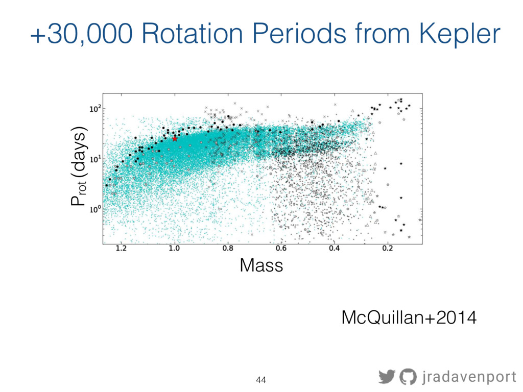
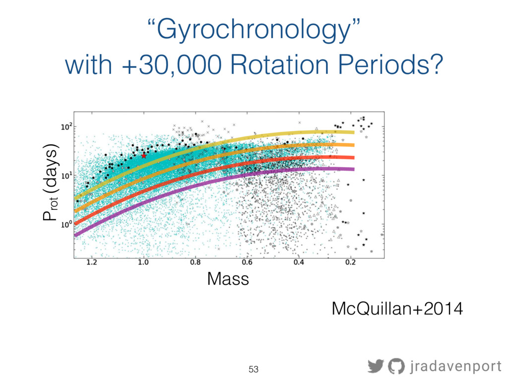
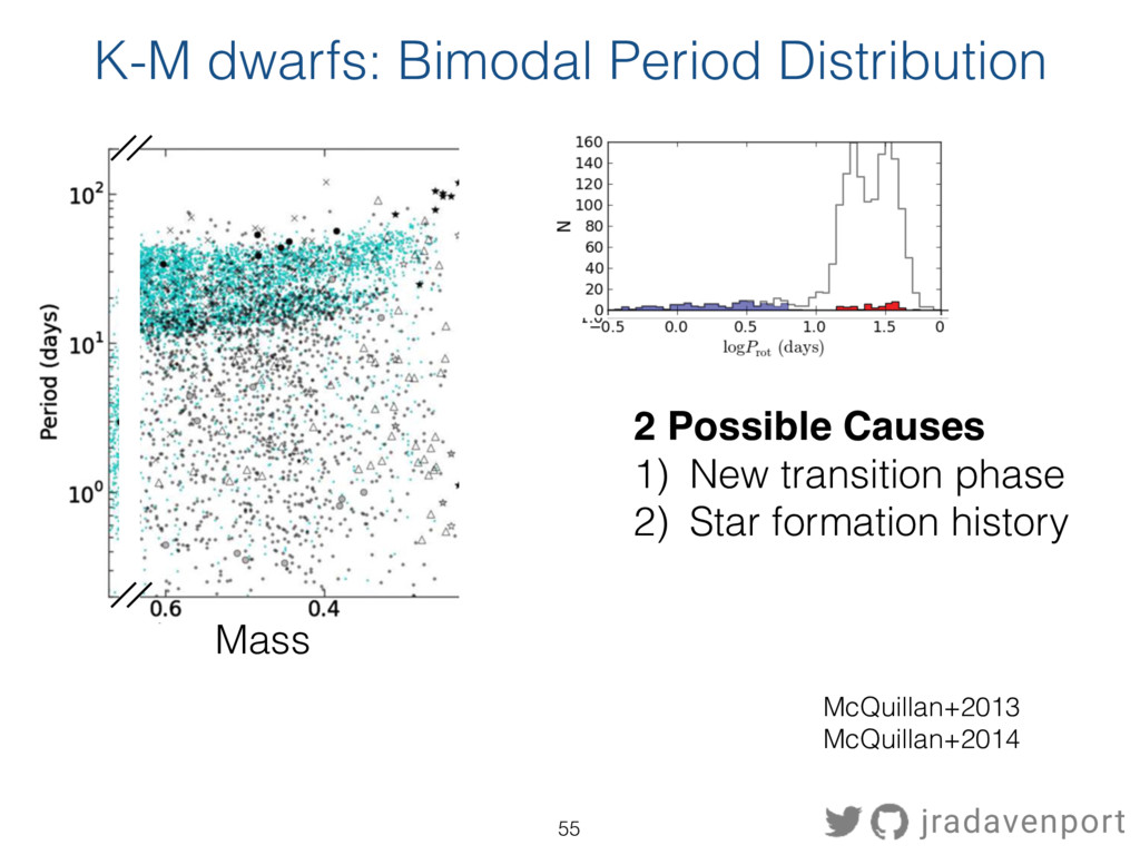
55. 4 April McQuillan, Mazeh, & Aigrain measurements. The 34,030 new rotation periods derived using AutoACF are shown as cyan as described in the text. This figure also displays periods from Baliunas et al. (1996) and 2011; 41 stars), with gray and black symbols representing objects with young and old disk tional M-dwarf periods from the WFCAM Transit Survey (Goulding et al. 2012), for which from Pecaut & Mamajek (2013). Also included are periods from (Hartman et al. 2011; 1686 s of Baraffe et al. (1998), and periods from (Harrison et al. 2012; 265 crosses), with masses ann (1995), and the isochrones of Baraffe et al. (1998). l Journal Supplement Series, 211:24 (14pp), 2014 April McQuillan, Maze . mass with comparison to previous rotation period measurements. The 34,030 new rotation periods derived using AutoACF are as derived using the models of Baraffe et al. (1998), as described in the text. This figure also displays periods from Baliunas et 2007; 114 circles) and MEarth data from Irwin et al. (2011; 41 stars), with gray and black symbols representing objects with youn vely, all of which have available mass estimates. Additional M-dwarf periods from the WFCAM Transit Survey (Goulding et al. 20 fication is available (65 triangles), with masses derived from Pecaut & Mamajek (2013). Also included are periods from (Hartman et with mass estimates obtained using Teff and the models of Baraffe et al. (1998), and periods from (Harrison et al. 2012; 265 crosses K to Teff conversion using data from Kenyon & Hartmann (1995), and the isochrones of Baraffe et al. (1998). K-M dwarfs: Bimodal Period Distribution Mass 1212 A. McQuillan, S. Aigrain and T. Mazeh Figure 9. Period versus amplitude for the rotating Kepler field M dwarfs. The blue dots represent objects with Prot < 10 d, whi stable modulation patterns in their light curves, and blue stars known, short-period eclipsing binaries (Prˇ sa et al. 2011). The red do of candidate transiting planets (Batalha et al. 2013). All the other M dwarfs with detected rotation periods are shown as grey dot parameter are shown along the corresponding axis, with matching colours. Two long-period binaries are not shown as blue stars in t Figure 9. Period versus amplitude for the rotating Kepler field M dwarfs. The blue dots represent objects with Prot < 10 d, whi stable modulation patterns in their light curves, and blue stars known, short-period eclipsing binaries (Prˇ sa et al. 2011). The red do of candidate transiting planets (Batalha et al. 2013). All the other M dwarfs with detected rotation periods are shown as grey dot parameter are shown along the corresponding axis, with matching colours. Two long-period binaries are not shown as blue stars in t Figure 10. Period versus effective temperature for the rotating Kepler field Figure 11. Histogram of the short- and long-pe McQuillan+2013 McQuillan+2014 2 Possible Causes 1) New transition phase 2) Star formation history jradavenport 55
56. Davenport 2017 Use Gaia DR1 to filter out subgiants Select only main sequence jradavenport 56
57. before after Davenport 2017 Rotation Bimodality: all nearby dwarf stars! MS-filtered 600 Myr “gyrochrone” Crude gyrochonology for field stars! jradavenport 57
58. Next: Extend to K2 & TESS (+Gaia) • How localized is the bimodality? • Star formation history on small scales? • Effects of spiral arms visible? Davenport + Angus (2018?) jradavenport 58
59. 59 Summary: Stellar Magnetism with Kepler A revolution for flare studies Flare rates do change with stellar age! jradavenport HAT-P-11: Evidence for a Solar-like Dynamo 15 Figure 9. Spots detected on HAT-P-11 with STSP (see Section 3). The radius of each circle corresponds to the size of the spot. The shading beneath corresponds to the number of times the planet occulted that spatial bin on the stellar surface, which can be used as a proxy for relative completeness. Note that the spots occur preferentially at two active latitudes near ±15 . The 6:1 period commensurability between the orbital period and stellar rotation period produces the alternating longitudinal stripes in relative occultation number. The two red circles in the western hemisphere near longitude 90 highlight the spots derived from the transit light curve in Figure 8, and the four blue circles in the eastern hemisphere near longitude 30 correspond to the spots derived from the transit light curve in Figure 6. The green circle near longitude 100 corresponds to the large spot discussed in Figure 13. for the sensitivities and biases of the di↵erent observing methods is beyond the scope of this paper. The latitude distribution of spots of HAT- P-11 and four years of solar observations are shown in Figure 10. The four-year span of solar observations closely resembles the mean spot latitudes and standard deviation of spot latitudes that we measure for HAT-P-11. The sunspots included in Figure 10 span the active maximum of solar Cycle 19, which was the so- lar maximum with the largest recorded num- ber of spots since telescopic observations began (Solanki et al. 2013). show the mean latitudes of spots on each hemi- sphere of the Sun, and the standard deviations of the spot distributions. The pattern of the solar activity cycle is visible — sunspots in the beginning of the cycle appear in small numbers at high latitudes, then large numbers near 15 , before settling back to lower numbers near the equator. The standard deviations of the spot distributions are correlated with the mean lat- itude — the active latitudes are broadest at the beginning of the activity cycle when spots form at high latitudes, and the active latitudes become narrower as they approach the equator later in the activity cycle. The combined e↵ect Detailed starspot properties for some systems! +30k stellar rotation periods Field gyrochronology possible!