ESTRUTURAS DE DADOS PROBABILÍSTICAS PARA REPRESENTAÇÃO DE GRAFOS GIGANTES

Transcript

1. ESTRUTURAS DE DADOS PROBABILÍSTICAS PARA REPRESENTAÇÃO DE GRAFOS GIGANTES Juan P. A. Lopes, Fabiano S. Oliveira*, Paulo E. D. Pinto*, Valmir C. Barbosa 28 de novembro de 2018
2. Agenda Motivation Probabilistic Representations Graph Streams 2 Outlook
3. Motivation Why are sketching data structures relevant to graph problems? 3
4. Some real-life graphs are massive Observing global structures is hard 2.2 billion 128 MB 66 billion 23 billion 100’s of billions Number of connected devices, 2018. https://www.statista.com/statistics/471264/iot- number-of-connected-devices-worldwide/ Internet Estimated number of directed edges, 2018. http://files.shareholder.com/downloads/AMD A-2F526X/5887909887x0x961126/1C3B57 60-08BC-4637-ABA1-A9423C80F1F4/Q31 7_Selected_Company_Metrics_and_Financia ls.pdf Twitter Number of active users, 2018. https://www.statista.com/statistics/264810/number-of-monthl y-active-facebook-users-worldwide/ Facebook Typical amount of RAM in a typical router. Routers Number of basepairs in a typical metagenomic sample. https://arxiv.org/abs/1112.4193 Metagenomic assemblies 4
5. Memory is limited Too many vertices Even sparse graphs with hundreds of billions of vertices may have a hard time fitting in main memory. Too many edges The amount of memory needed to represent dense graphs grow quadratically with the number of vertices. Limited hardware Modern IoT setups sometimes rely on hardware with limited amount of resources to spare in a graph processing application. Graphs are getting bigger 5
6. 6 SKETCHING DATA STRUCTURES also known as Probabilistic Data Structures
7. Metagenomic assembly De novo assembly of genomes from short-reads in metagenomic samples. • A read is a variable-length fragment of larger genomes. • Each read is broken down into fixed-length strings: a k-mer. • Those k-mers define a de Bruijn graph. 7 Pell, Jason, et al. (2012). Scaling metagenome sequence assembly with probabilistic de Bruijn graphs. Proceedings of the National Academy of Sciences. ...GTCATACTACGATACATAACTAGACTAGACTAAGACATACGATA... GTCATACTA ATACTACGATA ATACATAACTA CTAGACTAGACTAAGAC AAGACATACGATA 1. Sample 2. Short-reads 3. K-mers ATACTACGATA ATACTAC TACTACG ACTACGA CTACGAT TACGATA GTCATACTA GTCATAC TCATACT CATACTA 4. de Bruijn graph ATACTAC …G …A …T …A C… T… G…
8. Metagenomic assembly De novo assembly of genomes from short-reads in metagenomic samples. • The good: you do not really need to store edges. • The bad: O(4k) vertices. Human genome alone: 512GB. Problem: to find components in the graph created from a metagenomic sample. 8 Pell, Jason, et al. (2012). Scaling metagenome sequence assembly with probabilistic de Bruijn graphs. Proceedings of the National Academy of Sciences. 4. De Bruijn graph ATACTAC T… G… C… A… …T …G …C …A
9. Bloom filter Represents sets, allowing membership tests with a probability of false positives. • There are no false negatives; • 10 bits per element are enough to ensure for a probability of false positives of less than 1%. • Some applications can handle as high as 15% f.p., requiring less than 4 bits per element. 0 1 0 0 1 1 1 0 0 1 0 0 1 0 0 1 h 1 (x) h 3 (x) h 2 (x) 9 Bloom, B. H. (1970). Space/time trade-offs in hash coding with allowable errors. Communications of the ACM. ATACTAC
10. Not only theory This is production-ready Open-Source Software! Data Intensive Biology Lab, UC Davis School of Veterinary Medicine
11. Probabilistic Implicit Representations Use less memory by allowing errors 11
12. Space Optimal Representations General Graphs Trees Complete Graphs Adjacency Matrix: O(n2) Adjacency List: O(m log n) • A representation is said to be space optimal if it requires O(f(n)) bits to represent a class containing 2ϴ(f(n)) graphs on n vertices; • Optimality depends on the represented class. 12 Spinrad, J. P. (2003). Efficient graph representations. American Mathematical Society.
13. Space Optimal Representations 2ϴ(n log n) members: • Trees; • Interval graphs; • Planar; • Complete graphs; • ... 13 Spinrad, J. P. (2003). Efficient graph representations. American Mathematical Society. 2ϴ(n²) members: • General graphs; • Bipartites/co-bipartite; • Split; • Chordal; • Comparability; • ...
14. 3 2 1 Space Optimal Representations • A representation is said to be space optimal if it requires O(f(n)) bits to represent a class containing 2ϴ(f(n)) graphs on n vertices; • We could just enumerate all labelled graphs and use that as optimal representation. 14 Spinrad, J. P. (2003). Efficient graph representations. American Mathematical Society. A A B A B C 4 A B C 5 A B C 6 A B C . . .
15. Implicit Representations A representation is said to be implicit if it has the following properties: Space optimal O(f(n)) bits to represent a class containing 2ϴ(f(n)) graphs on n vertices; Distributes information Each vertex stores O(f(n)/n) bits; Local adjacency test Only local vertex information is required to test adjacency; 15 Spinrad, J. P. (2003). Efficient graph representations. American Mathematical Society.
16. Probabilistic Implicit Representations Space optimal O(f(n)) bits to represent a class containing 2ϴ(f(n)) graphs on n vertices; Distributes information Each vertex stores O(f(n)/n) bits; Local adjacency test Only local vertex information is required to test adjacency; For probabilistic implicit representations, we introduce a fourth property: Probabilistic adjacency test Constant relative probability of false positives or false negatives. 16
17. Bloom filter Idea: to replace each vertex set in an adjacency list with a Bloom filter. • Each edge would require only O(1) bits, instead of O(log n); • By using Bloom filters, there would be no false negatives, only false positives. • Similarly, a single Bloom filter could be used to store the entire edge set, but technically this would not be an implicit representation. 1 2 3 4 5 2 1 3 2 2 4 1 3 3 5 REGULAR ADJACENCY LIST 1 2 3 4 5 0 BLOOM FILTER REPRESENTATION 1 1 0 1 0 1 1 0 1 1 1 0 1 1 0 0 1 0 1 17
18. MinHash Represents sets through a constant-sized signature and allow computing the Jaccard coefficient between two or more sets. 6 MinHash(A) 71 57 106 81 MinHash(B) 80 34 73 88 6 71 57 106 81 80 73 88 11 6 1 34 11 6 1 34 h 1 h 2 h 3 h 4 h 5 h 6 h 7 h 8 18 Broder, A. Z. (1997). On the resemblance and containment of documents. In Compression and complexity of sequences. Charikar, Moses S. (2002). Similarity estimation techniques from rounding algorithms. Proceedings of STOC’02. • This is known as a Locality-Sensitive Hashing (LSH). • Similar techniques encode other metrics, e.g. Charikar Signatures (SimHash) encode cosine distance.
19. MinHash Idea: construct a set for each vertex, such that the Jaccard index between any pair of vertices encodes their adjacency. 19 {1, 2, 3, 4} {1, 3, 4, 6} {1, 2, 3, 4} {4, 6, 7, 9}
20. MinHash Idea: construct a set for each vertex, such that the Jaccard index between any pair of vertices encodes their adjacency. 0 1 δ A δ B 20
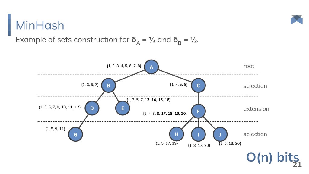
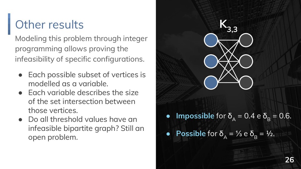
21. MinHash Example of sets construction for δ A = ⅓ and δ B = ½. A C B {1, 2, 3, 4, 5, 6, 7, 8} D E F G {1, 3, 5, 7} {1, 4, 5, 8} {1, 3, 5, 7, 9, 10, 11, 12} {1, 3, 5, 7, 13, 14, 15, 16} {1, 4, 5, 8, 17, 18, 19, 20} {1, 5, 9, 11} root selection extension selection H I J {1, 5, 17, 19} {1, 8, 17, 20} {1, 5, 18, 20} O(n) bits 21
22. Experimental Results For MinHash-based representation 1 Increasing the threshold seems to increase the rate of false negatives and decrease false positives. 2 The perfect threshold depends on the application tolerance for false positives and false negatives. 3 Observations The experiment was run with k=128 hash functions and a graph with n=200 vertices. 22
23. Experimental Results For MinHash-based representation 1 Increasing the signature size seems to have more effect on the rate of false negatives than positives. 2 This effect appears the same for whatever choice of threshold. 3 Observations The experiment was run with δ = 0.375 and a graph with n=200 vertices. 23
24. Other results Any efficient representation for bipartite, co-bipartite or split graphs can be used to represent general graphs efficiently. 1 3 2 5 4 1 2 3 4 5 1 2 3 4 5 24 Spinrad, J. P. (2003). Efficient graph representations. American Mathematical Society.
25. Other results Modeling this problem through integer programming allows proving the infeasibility of specific configurations. x A x AB S A S B S C x B x C x AC x BC x ABC A B C • Each possible subset of vertices is modelled as a variable. • Each variable describes the size of the set intersection between those vertices. 25
26. Other results Modeling this problem through integer programming allows proving the infeasibility of specific configurations. • Each possible subset of vertices is modelled as a variable. • Each variable describes the size of the set intersection between those vertices. • Do all threshold values have an infeasible bipartite graph? Still an open problem. K 3,3 • Impossible for δ A = 0.4 e δ B = 0.6. • Possible for δ A = ⅓ e δ B = ½. 26
27. Wrapping up this section Other graph classes? It seems plausible that other classes with 2ϴ(n log n) graphs should probably admit efficient probabilistic representations. Any class with 2ϴ(n²) graphs? Finding such class could prove this technique useful even for relatively small graphs. Bipartite, co-bipartite, or split? Proving that would imply the existence of an efficient probabilistic representation in O(n) bits for all graphs. Some open questions 27 This work was awarded as one of the top 9 master’s thesis of 2017 in a contest held by the Brazilian Computer Society (SBC).
28. Graph Streams How to represent dynamic graphs in sublinear space? 28
29. Graph Streams Graph Streams are graphs represented in the data stream model, i.e. single-pass through a stream of edge insertions and deletions. Problem: compute parameters with restricted space. A B C E D F +DF, -BC, +BE, +AC +BC, -DF, -BD, +AE 29 McGregor, A. (2014). Graph stream algorithms: a survey. ACM SIGMOD.
30. Graph Streams Graph Streams are graphs represented in the data stream model, i.e. single-pass through a stream of edge insertions and deletions. Problem: compute parameters with restricted space. McGregor, A. (2014). Graph stream algorithms: a survey. ACM SIGMOD. 30
31. Graph Streams Is it possible to check if the graph is connected in a streaming model? Can we sample a full spanning forest using O(n logc n) bits? A B C E D F 31 This is trivial for insert-only streams
32. Graph Streams Idea: we can sample an edge from each vertex and merge its endpoints in a single “super-vertex”. Repeat. This procedures finishes in O(log n) steps. A B C E D F 32 Ahn, K. J., Guha, S., and McGregor, A. (2012). Analyzing graph structure via linear measurements. Proceedings of SODA’12.
33. Graph Streams Idea: we can sample an edge from each vertex and merge its endpoints in a single “super-vertex”. Repeat. This procedures finishes in O(log n) steps. A B C E D F 33 Ahn, K. J., Guha, S., and McGregor, A. (2012). Analyzing graph structure via linear measurements. Proceedings of SODA’12.
34. Graph Streams Idea: we can sample an edge from each vertex and merge its endpoints in a single “super-vertex”. Repeat. This procedures finishes in O(log n) steps. A B C E D F 34 Ahn, K. J., Guha, S., and McGregor, A. (2012). Analyzing graph structure via linear measurements. Proceedings of SODA’12.
35. Graph Streams A simpler problem: Is it possible to sample a random edge from any cut-set [S, V\S] in a graph stream storing O(n logc n) bits? A B C E D F 35 Ahn, K. J., Guha, S., and McGregor, A. (2012). Analyzing graph structure via linear measurements. Proceedings of SODA’12.
36. Sampling edges from cut-set Idea: to represent graph through a modified incidence matrix, where each edge has value 1 or -1, depending on which vertex is the endpoint. A B C E D F 36 A B C D E F 1 1 0 0 0 0 0 0 AB AC BD BE CD CE CF DF -1 0 1 1 0 0 0 0 0 -1 0 0 1 1 1 0 0 0 -1 0 -1 0 0 1 0 0 0 -1 0 -1 0 0 0 0 0 0 0 0 -1 -1
37. Sampling edges from cut-set The main benefit from this representation is the ability to sum incidence vectors to find the corresponding vector of a cut-set. Being able to sample nonzero coordinates from this vector implies sampling edges from such cut-set. A B C E D F 37 A +B +D A+B+D 1 1 0 0 0 0 0 0 AB AC BD BE CD CE CF DF -1 0 1 1 0 0 0 0 0 0 -1 0 -1 0 0 1 0 1 0 1 -1 0 0 1
38. What is ℓ 0 -sampling? Sampling, with uniform probability, of a nonzero coordinate from a vector a, represented incrementally by a stream of updates. • Some updates may cancel others; • Must be done in sublinear space; • Known lower-bound: Ω(log2 n). Cormode, G., Muthukrishnan, S., and Rozenbaum, I. (2005). Summarizing and mining inverse distributions on data streams via dynamic inverse sampling. In Proceedings of VLDB’05. Jowhari, H., Saglam, M., and Tardos, G. (2011). Tight bounds for lp-samplers, finding duplicates in streams, and related problems. In Proceedings of PODS’11. 1 0 8 -4 0 -7 -15 9 -1 0 1 a 2 3 4 5 6 7 8 9 10 (3, +8) (1, +1) (4, -4) (9, +3) (10, -5) (10, -1) 38
39. What is ℓ 0 -sampling? Sampling, with uniform probability, of a nonzero coordinate from a vector a, represented incrementally by a stream of updates. • Some updates may cancel others; • Must be done in sublinear space; • Known lower-bound: Ω(log2 n). Cormode, G., Muthukrishnan, S., and Rozenbaum, I. (2005). Summarizing and mining inverse distributions on data streams via dynamic inverse sampling. In Proceedings of VLDB’05. Jowhari, H., Saglam, M., and Tardos, G. (2011). Tight bounds for lp-samplers, finding duplicates in streams, and related problems. In Proceedings of PODS’11. 1 0 8 -4 0 -7 -15 9 -1 0 1 a 2 3 4 5 6 7 8 9 10 39
40. Sampling edges from cut-set Is it possible to encode each incidence vector in a compact representation? random projection 0 0 1 -1 0 0 -1 1 -1 1 0 0 0 0 1 -1 ℓ 0 -sampler 40
41. ℓ 0 -sampling algorithm Assign each coordinate a random bucket Use hash functions. Each bucket must have exponentially decreasing probabilities of representing each coordinate. Find 1-sparse vector There is a high probability that at least one bucket will represent a 1-sparse vector, that is, a vector with a single nonzero coordinate. Recover its only nonzero coordinate Through a randomized procedure called 1-sparse recovery, it is possible to recover the nonzero coordinates from 1-sparse vectors, using O(log n) bits. The sampling algorithm is based on the following idea: 41
42. 1-sparse recovery Tests if a vector is 1-sparse. If yes, it recovers the single nonzero coordinate. linear transform not 1-sparse yes no 100% sure prob. ≥ 1 - n/p b 0 b 1 b 2 z O(log n) bits 42
43. Variant (a) Variant (b) p=1/4 p=1/2 p=1/8 p=1/16 p=2-m 1 2 3 4 m (u i ,Δ i ) h(u i ) p=1/2 p=1/8 p=1/16 p=2-m p=1/4 1 2 3 4 m (u i ,Δ i ) h j (u i ) • Single hash function (more efficient); • Non-independent buckets. • Multiple hash function; • Independent buckets (easier). 43
44. ℓ 0 -sampling algorithm Two distinct probabilities 44 probability of representing a 1-sparse subvector probability of being chosen to represent a coordinate
45. ℓ 0 -sampling algorithm 1 It is easy to see that for every value of r, there will always be a bucket with high probability of recovery (~0.35). 2 There will also be other adjacent buckets with high probability of recovery. 3 Observations We define r, the number of nonzero coordinates in a vector. p i is the probability of the ith bucket being 1-sparse. r = 200 r = 4096 r = 10.000.000 45
46. ℓ 0 -sampling algorithm m = ⌈log 2 n + 5⌉ is enough to ensure a probability of failure of less than 0.31. analyzing factors’ maxima 46
47. Experimental results Correcly sized setup. Variant (a) Variant (b) 1 Variants behave similarly, with error apparently constant under 20% in both tests. 2 The distribution of sampled coordinates (not shown) was also similar in both tests. 3 Observations We tested both variants in a correctly sized setup, i.e. r ≤ 4096, m = 17. 47
48. Experimental results Undersized setup. Variant (a) Variant (b) 1 Variants behave similarly, with error growing from under 20% to almost 100% in both tests. 2 The distribution of sampled coordinates (not shown) was also similar in both tests. 3 Observations We tested both variants in an undersized setup, i.e. r ≤ 4096, m = 10. 48
49. Outlook What should we expect from sketching data structures in a near future? 49
50. In this talk... Bloom Filter Adjacency test on general graphs in O(m) bits. Specially useful for sparse massive graphs. Has constant probability of false positives. No false negatives. MinHash Adjacency test on trees in O(n) bits. Better space complexity than the optimal deterministic representation. Useful for giant trees (over a billion nodes). ℓ 0 -Sampler Dynamic spanning forest in O(n log3 n) bits. Useful for very dense graphs. … I presented the application of three sketching data structures for massive graph problems. # 50
51. Not only a theory. Not only for graphs. Sketching data structures are growing Mash: Fast genome and metagenome distance estimation using MinHash. Redis PFCOUNT: set distinct count using HyperLogLog. MMDS book chapter 4: several sketch-based stream algorithms. 51
52. Our next steps ℓ 0 -Sampler The ability to sample edges from cut-sets is very useful and can help to produce many new graph algorithms. We are searching for new algorithms that use ℓ 0 -sampling as a primitive 52
53. Questions? Slidedeck available at: juanlopes.net/ac18 53