Monopoly and Contestability 8.1.1 Fixed Costs versus Sunk Costs 8.1.2 Contestability 8.1.3 War of Attrition 3 8.2 Sunk Costs and Barriers to Entry: The Stackelberg-Spence-Dixit Model 8.2.1 Accommodated, Deterred, and Blockaded Entry 8.2.2 Discussion and Extensions (The Spence Dixit model) 8.2.3 Other Forms of Capital 2 / 36
8.1.1 Fixed Costs versus Sunk Costs 8.1.2 Contestability 8.1.3 War of Attrition 3 8.2 Sunk Costs and Barriers to Entry: The Stackelberg-Spence-Dixit Model 8.2.1 Accommodated, Deterred, and Blockaded Entry 8.2.2 Discussion and Extensions (The Spence Dixit model) 8.2.3 Other Forms of Capital 3 / 36
zero profit. • However, the profit rate is systematically greater in certain industries then in others. • In order to explain this, some type of restriction to entry must exist in these industries to prevent other firms from taking advantage of the profitable market situations. • We consider barriers to entry not created by government. 4 / 36
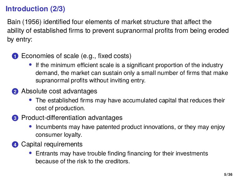
that affect the ability of established firms to prevent supranormal profits from being eroded by entry: 1 Economies of scale (e.g., fixed costs) • If the minimum efficient scale is a significant proportion of the industry demand, the market can sustain only a small number of firms that make supranormal profits without inviting entry. 2 Absolute cost advantages • The established firms may have accumulated capital that reduces their cost of production. 3 Product-differentiation advantages • Incumbents may have patented product innovations, or they may enjoy consumer loyalty. 4 Capital requirements • Entrants may have trouble finding financing for their investments because of the risk to the creditors. 5 / 36
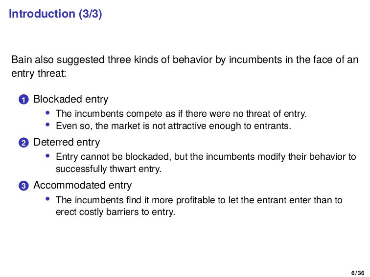
incumbents in the face of an entry threat: 1 Blockaded entry • The incumbents compete as if there were no threat of entry. • Even so, the market is not attractive enough to entrants. 2 Deterred entry • Entry cannot be blockaded, but the incumbents modify their behavior to successfully thwart entry. 3 Accommodated entry • The incumbents find it more profitable to let the entrant enter than to erect costly barriers to entry. 6 / 36
8.1.1 Fixed Costs versus Sunk Costs 8.1.2 Contestability 8.1.3 War of Attrition 3 8.2 Sunk Costs and Barriers to Entry: The Stackelberg-Spence-Dixit Model 8.2.1 Accommodated, Deterred, and Blockaded Entry 8.2.2 Discussion and Extensions (The Spence Dixit model) 8.2.3 Other Forms of Capital 7 / 36
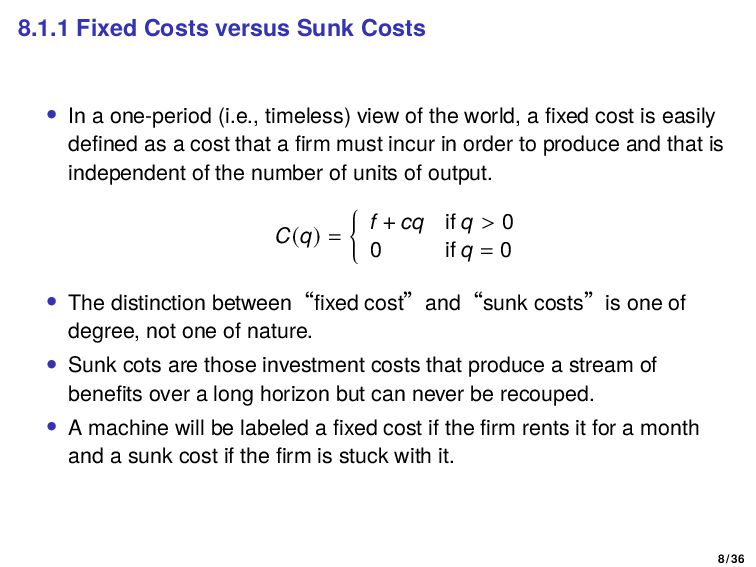
(i.e., timeless) view of the world, a fixed cost is easily defined as a cost that a firm must incur in order to produce and that is independent of the number of units of output. C(q) = { f + cq if q > 0 0 if q = 0 • The distinction between“fixed cost”and“sunk costs”is one of degree, not one of nature. • Sunk cots are those investment costs that produce a stream of benefits over a long horizon but can never be recouped. • A machine will be labeled a fixed cost if the firm rents it for a month and a sunk cost if the firm is stuck with it. 8 / 36
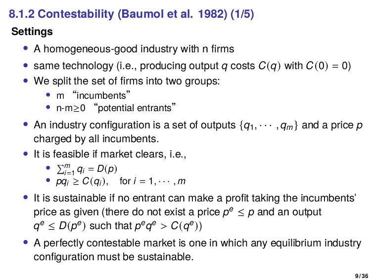
homogeneous-good industry with n firms • same technology (i.e., producing output q costs C(q) with C(0) = 0) • We split the set of firms into two groups: • m “incumbents” • n-m≥0 “potential entrants” • An industry configuration is a set of outputs {q1, · · · , qm } and a price p charged by all incumbents. • It is feasible if market clears, i.e., • ∑ m i=1 qi = D(p) • pqi ≥ C(qi ), for i = 1, · · · , m • It is sustainable if no entrant can make a profit taking the incumbents’ price as given (there do not exist a price pe ≤ p and an output qe ≤ D(pe) such that peqe > C(qe)) • A perfectly contestable market is one in which any equilibrium industry configuration must be sustainable. 9 / 36
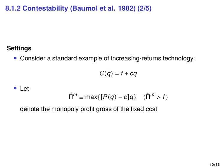
a standard example of increasing-returns technology: C(q) = f + cq • Let ˜ Πm ≡ max{[P(q) − c]q} (˜ Πm > f) denote the monopoly profit gross of the fixed cost 10 / 36
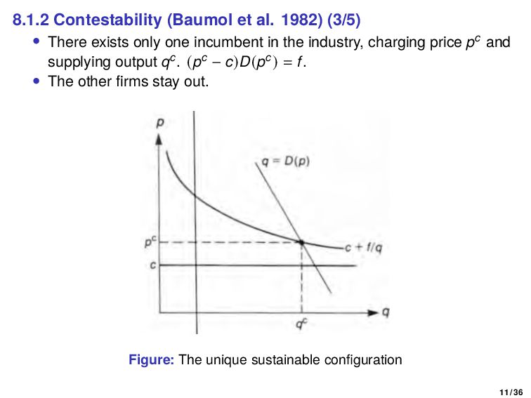
only one incumbent in the industry, charging price pc and supplying output qc. (pc − c)D(pc) = f. • The other firms stay out. Figure: The unique sustainable configuration 11 / 36
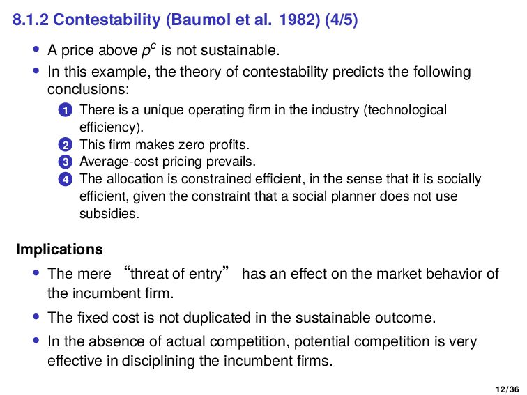
above pc is not sustainable. • In this example, the theory of contestability predicts the following conclusions: 1 There is a unique operating firm in the industry (technological efficiency). 2 This firm makes zero profits. 3 Average-cost pricing prevails. 4 The allocation is constrained efficient, in the sense that it is socially efficient, given the constraint that a social planner does not use subsidies. Implications • The mere “threat of entry” has an effect on the market behavior of the incumbent firm. • The fixed cost is not duplicated in the sustainable outcome. • In the absence of actual competition, potential competition is very effective in disciplining the incumbent firms. 12 / 36
entrants have the same cost function as incumbents. • Prices adjust more slowly than decisions about quantities or entry. • Entry costs are not sunk costs and can be recovered upon exit. By these assumptions, entrants can do “hit-and-run entry.” • Suppose the incumbent’s price is rigid for a length of time 𝜏. • If the incumbent’s price exceeds pc, an entrant can enter, undercut pc slightly, and exit the industry before 𝜏 units of time having elapsed. • Thus, only price pc is sustainable. 13 / 36
adjustments take place more quickly than quantity adjustments. • Two firms fight for control of an increasing-returns industry. • Duopoly competition may be costly because it generates negative profits. • The object of the fight is to induce the rival to give up. • The winning firm obtains monopoly power. • The loser is left wishing it had never entered the fight. • If at some point in time his rival has not yet quit, a player gives up. 14 / 36
continuous from 0 to ∞. • The rate of interest is r. • There are two firms, with identical cost functions: C(q) = { f + cq if q > 0 0 if q = 0 • If the two firms are in the market at time t, price equals marginal cost c and each firm loses f per unit of time. • If only one firm is in the market, the price is equal to the monopoly price, pm, and the firm makes instantaneous profit ˜ Πm − f > 0. • At each instant, each firm decides whether to exit (conditional on the other firm’s still being in the market at that date). • Exit is costless. • The remaining firm stays in forever after its rival has dropped out. 15 / 36
be indifferent, the expected profits from the two actions must be the same. • If both firms are still in the market at date t, each firm drops out with probability: xdt (between t and t+dt), where x ≡ rf ˜ Πm − f . • Firm 1 is indifferent between dropping out at date t and staying until t + dt if 0 = −fdt + (xdt) [ ˜ Πm − f r ] + 0. • Each firm drops out according to a Poisson process with parameter x. • The equilibrium is not unique. 16 / 36
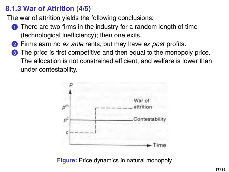
the following conclusions: 1 There are two firms in the industry for a random length of time (technological inefficiency); then one exits. 2 Firms earn no ex ante rents, but may have ex post profits. 3 The price is first competitive and then equal to the monopoly price. The allocation is not constrained efficient, and welfare is lower than under contestability. Figure: Price dynamics in natural monopoly 17 / 36
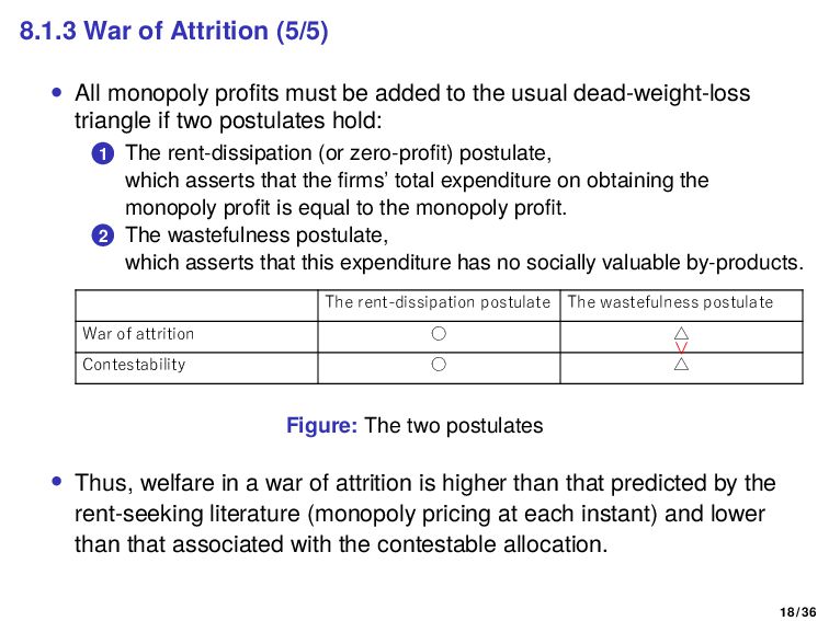
be added to the usual dead-weight-loss triangle if two postulates hold: 1 The rent-dissipation (or zero-profit) postulate, which asserts that the firms’ total expenditure on obtaining the monopoly profit is equal to the monopoly profit. 2 The wastefulness postulate, which asserts that this expenditure has no socially valuable by-products. The wastefulness postulate The rent-dissipation postulate △ ◦ War of attrition △ ◦ Contestability > Figure: The two postulates • Thus, welfare in a war of attrition is higher than that predicted by the rent-seeking literature (monopoly pricing at each instant) and lower than that associated with the contestable allocation. 18 / 36
8.1.1 Fixed Costs versus Sunk Costs 8.1.2 Contestability 8.1.3 War of Attrition 3 8.2 Sunk Costs and Barriers to Entry: The Stackelberg-Spence-Dixit Model 8.2.1 Accommodated, Deterred, and Blockaded Entry 8.2.2 Discussion and Extensions (The Spence Dixit model) 8.2.3 Other Forms of Capital 19 / 36
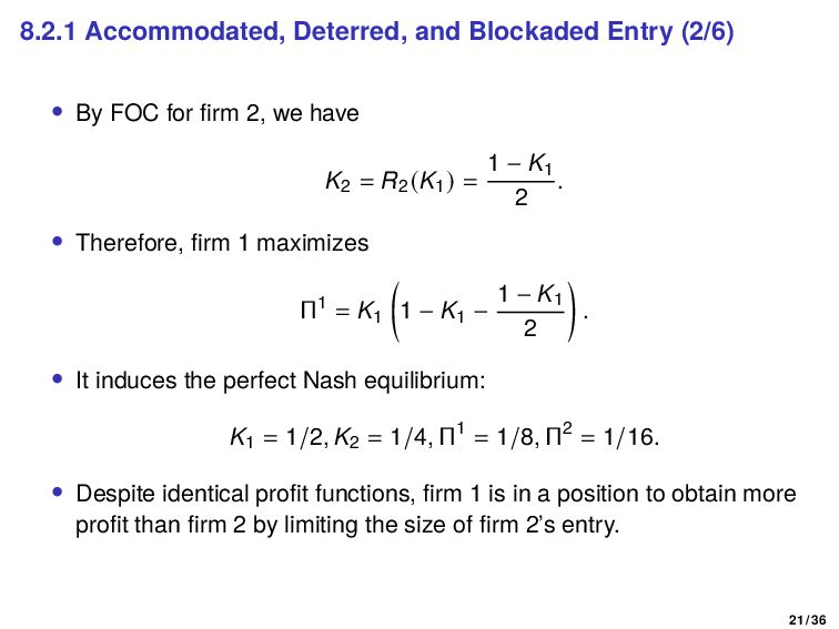
(1934) • Consider a two-firm industry. • Firm 1 (the incumbent) chooses a level of capital K1, which is fixed. • Firm 2 (the potential entrant) observes K1 and then chooses K2, which is fixed. • Assume that the profits of the two firms are specified by Π1(K1, K2 ) = K1 (1 − K1 − K2 ) Π2(K1, K2 ) = K2 (1 − K1 − K2 ). • Assume the following two properties, Πi j < 0 and Πi ij < 0 (the capital levels are strategic substitutes.) • Assume that there is no fixed cost of entry. • Firm 1 must anticipate the reaction of firm 2 to K1. 20 / 36
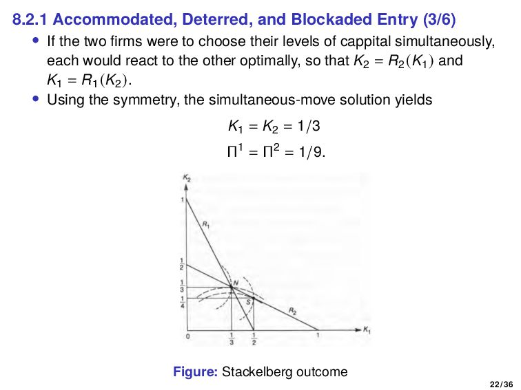
two firms were to choose their levels of cappital simultaneously, each would react to the other optimally, so that K2 = R2 (K1 ) and K1 = R1 (K2 ). • Using the symmetry, the simultaneous-move solution yields K1 = K2 = 1/3 Π1 = Π2 = 1/9. Figure: Stackelberg outcome 22 / 36
of the irreversibility of capital levels should be stressed. • Firm 1 is not on its reaction curve ex post; K1 = R1 (1/4) = 3 8 < 1 2 . • Firm 2 then choose K2 = R2 (3/8) = 5 16 > 1 4 . • In this sense, firm 1 loses by being flexible. • The fact that the investment cost is sunk is a barrier to exit and allows the incumbent to commit to a high capital level. • Hence, it is important that the capital investment be somewhat difficult to reverse if it is to have a commitment value. 23 / 36
and Porter (1977), we will show a barrier to mobility. • Firm 2 declines to enter (K2 = R2 (K1 ) = 0) only if K1 ≥ 1, which would yield negative profits to firm 1. • If firm 1 makes positive profits, firm 2 can choose a small level of capital, hardly affect the market price, and make a profit itself. • Such small-scale entry becomes unprofitable under increasing returns to scale. • Assume that firm 2 has the following profit function: Π2(K1, K2 ) = { K2 (1 − K1 − K2 ) − f if K2 > 0 0 if K2 = 0. Suppose that f < 1/16. 24 / 36
, the capital level that discourages entry, is given by max K2 [K2 (1 − K2 − Kb 1 ) − f] = 0, Kb 1 = 1 − 2 √ f > 1 2 . • When entry is deterred, the profit of firm 1 is Π1 = Kb 1 (1 − Kb 1 ) = (1 − 2 √ f)[1 − (1 − 2 √ f)] = 2 √ f (1 − 2 √ f). • If f is close to 1/16, this profit is greater than 1/8. • Accumulating beyond Kb 1 would reduce firm 1’s profit. • With f > 1/16, firm 1 blockades entry simply by choosing its monopoly capital level, Km 1 = 1/2. 25 / 36
use a model like Stackelberg but in capacities (instead of quantities), which allows a better understanding of three issues: 1 What does quantity competition mean? The profit functions represent reduced-form profit functions after one has solved for short-run product-market competition given the capacity levels. 2 Why does one of the firms enjoy a first-mover advantage? In quantities it did not make much sense, but if we think in capacities it could be that one of the firms obtained the technology first. 3 Why does quantity have a commitment value? In quantities this does not make much sense but in capacities, it makes all the sense because capacities are sunk. 26 / 36
compete in quantities in the short-run and in capacities in the long-run. Game: Stage 1: • Firm 1 (the incumbent) chooses capacity level K1 at a cost c0K1. • Firm 2 (the potential entrant) observes K1. Stage 2: • Both firms choose their outputs (q1, q2 ) simultaneously as well as their capacities ( ˜ K1, K2 ) where ˜ K1 ≥ K1. • Production involves cost c per unit of output. • Output cannot exceed capacity: qi ≤ Ki for all i. 27 / 36
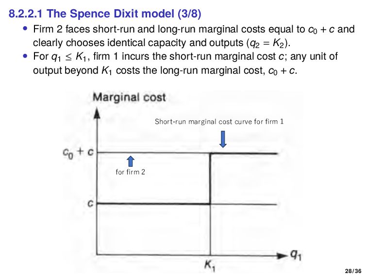
short-run and long-run marginal costs equal to c0 + c and clearly chooses identical capacity and outputs (q2 = K2). • For q1 ≤ K1, firm 1 incurs the short-run marginal cost c; any unit of output beyond K1 costs the long-run marginal cost, c0 + c. Short-run marginal cost curve for firm 1 for firm 2 28 / 36
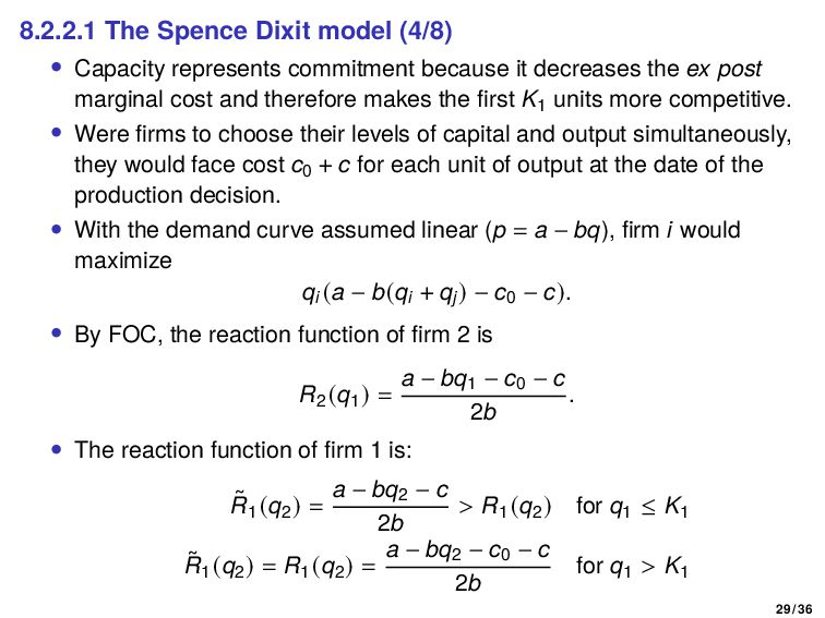
because it decreases the ex post marginal cost and therefore makes the first K1 units more competitive. • Were firms to choose their levels of capital and output simultaneously, they would face cost c0 + c for each unit of output at the date of the production decision. • With the demand curve assumed linear (p = a − bq), firm i would maximize qi (a − b(qi + qj ) − c0 − c). • By FOC, the reaction function of firm 2 is R2 (q1 ) = a − bq1 − c0 − c 2b . • The reaction function of firm 1 is: ˜ R1 (q2 ) = a − bq2 − c 2b > R1 (q2 ) for q1 ≤ K1 ˜ R1 (q2 ) = R1 (q2 ) = a − bq2 − c0 − c 2b for q1 > K1 29 / 36
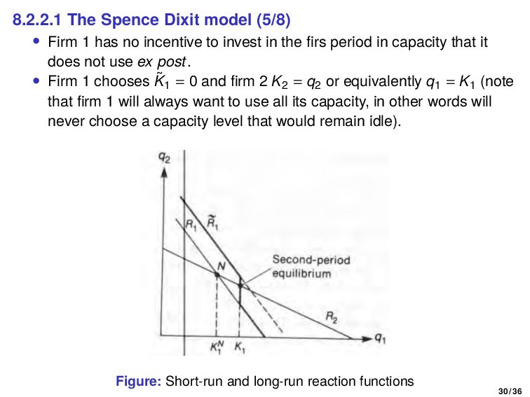
no incentive to invest in the firs period in capacity that it does not use ex post. • Firm 1 chooses ˜ K1 = 0 and firm 2 K2 = q2 or equivalently q1 = K1 (note that firm 1 will always want to use all its capacity, in other words will never choose a capacity level that would remain idle). Figure: Short-run and long-run reaction functions 30 / 36
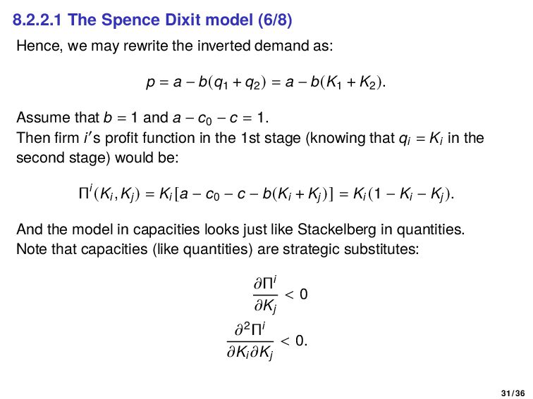
the inverted demand as: p = a − b(q1 + q2 ) = a − b(K1 + K2 ). Assume that b = 1 and a − c0 − c = 1. Then firm i′s profit function in the 1st stage (knowing that qi = Ki in the second stage) would be: Πi (Ki, Kj ) = Ki [a − c0 − c − b(Ki + Kj )] = Ki (1 − Ki − Kj ). And the model in capacities looks just like Stackelberg in quantities. Note that capacities (like quantities) are strategic substitutes: 𝜕Πi 𝜕Kj < 0 𝜕2Πi 𝜕Ki 𝜕Kj < 0. 31 / 36
reduced-form functions for price competition under capacity constraints allows us to perform some welfare analysis. • Let p = 1 − K1 − K2 denote the demand function. • Assume that the marginal cost is zero. The social optimum in this industry is to produce industry output K = 1. If p is the market price, the welfare loss from monopoly or duopoly pricing is equal to p2/2. K p 1 1 p 1-p DWL 0 32 / 36
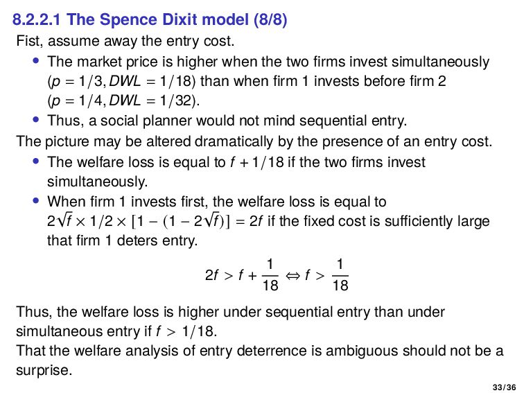
entry cost. • The market price is higher when the two firms invest simultaneously (p = 1/3, DWL = 1/18) than when firm 1 invests before firm 2 (p = 1/4, DWL = 1/32). • Thus, a social planner would not mind sequential entry. The picture may be altered dramatically by the presence of an entry cost. • The welfare loss is equal to f + 1/18 if the two firms invest simultaneously. • When firm 1 invests first, the welfare loss is equal to 2 √ f × 1/2 × [1 − (1 − 2 √ f)] = 2f if the fixed cost is sufficiently large that firm 1 deters entry. 2f > f + 1 18 ⇔ f > 1 18 Thus, the welfare loss is higher under sequential entry than under simultaneous entry if f > 1/18. That the welfare analysis of entry deterrence is ambiguous should not be a surprise. 33 / 36
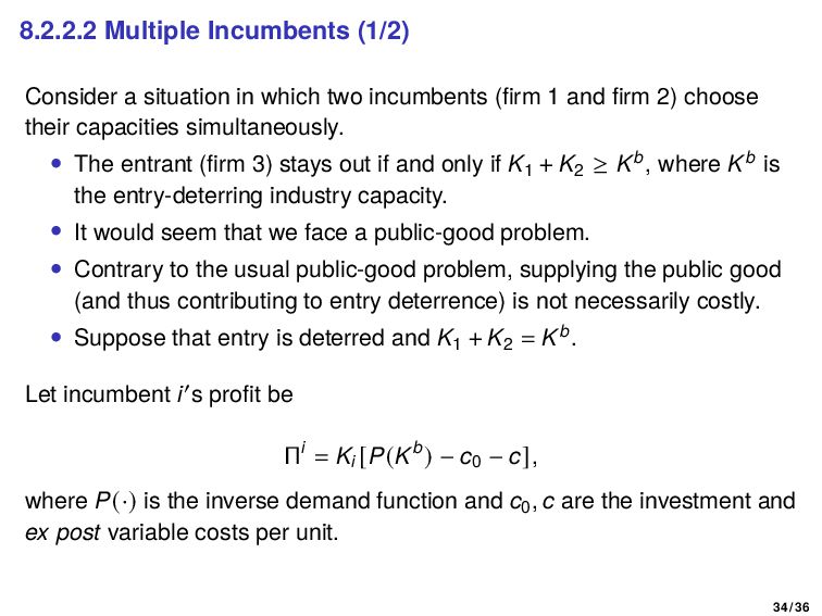
incumbents (firm 1 and firm 2) choose their capacities simultaneously. • The entrant (firm 3) stays out if and only if K1 + K2 ≥ Kb, where Kb is the entry-deterring industry capacity. • It would seem that we face a public-good problem. • Contrary to the usual public-good problem, supplying the public good (and thus contributing to entry deterrence) is not necessarily costly. • Suppose that entry is deterred and K1 + K2 = Kb. Let incumbent i′s profit be Πi = Ki [P(Kb) − c0 − c], where P(·) is the inverse demand function and c0, c are the investment and ex post variable costs per unit. 34 / 36
like to have the highest possible capital level: 𝜕Πi 𝜕Ki > 0 (∵ P(Kb) − c0 − c > 0). Hence, conditional on the actual deterrence of entry, each firm would like to contribute to entry deterrence as much as it can. Gilbert and Vives (1986) find that only overinvestment can occur. 35 / 36
have the same effect if they have commitment value (i.e., they are irreversible, at least in the short run). Consider the following three examples. 1 Learning by doing • The experience acquired by the established firms during previous production periods reduces their current production costs and thus may be considered to be a form of capital. • This gives the existing firms a competitive advantage, and it can discourage others from entering. 2 Developing a clientele • To develop a clientele is a capital decision that increases the demand for the product of the incumbent. • Advertising, promotional campaigns. To “preempt” demand. 3 Setting up a network of exclusive franchises • This is a capital decision that increases the entrant7s distribution costs. • The established supplier can assure himself of the services of the more capable franchisees by selecting them initially and imposing exclusivity on them. 36 / 36