Exploratory: An Introduction to Random Forest & Boruta

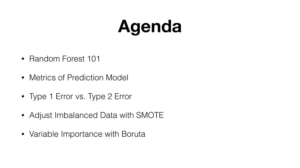
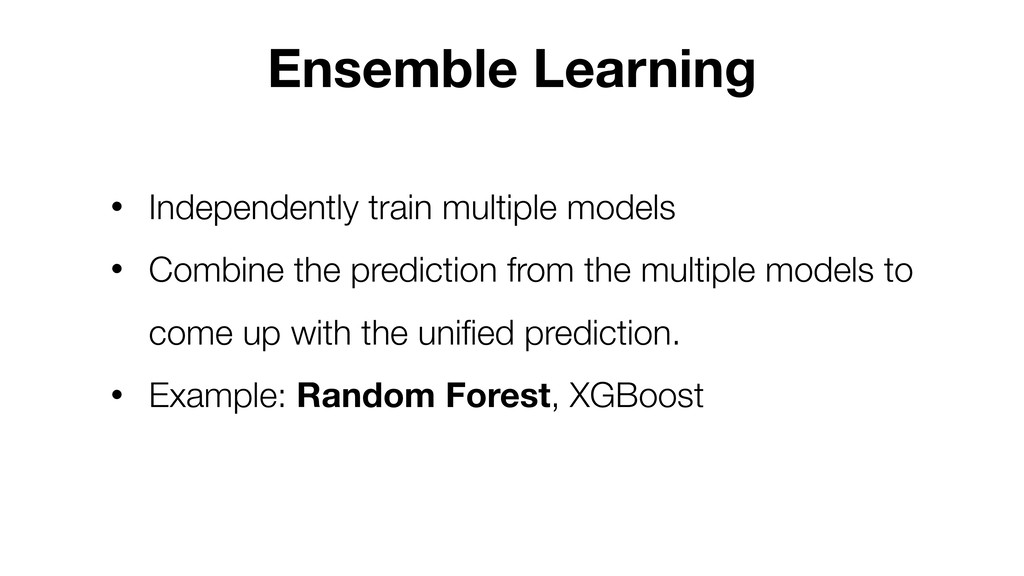
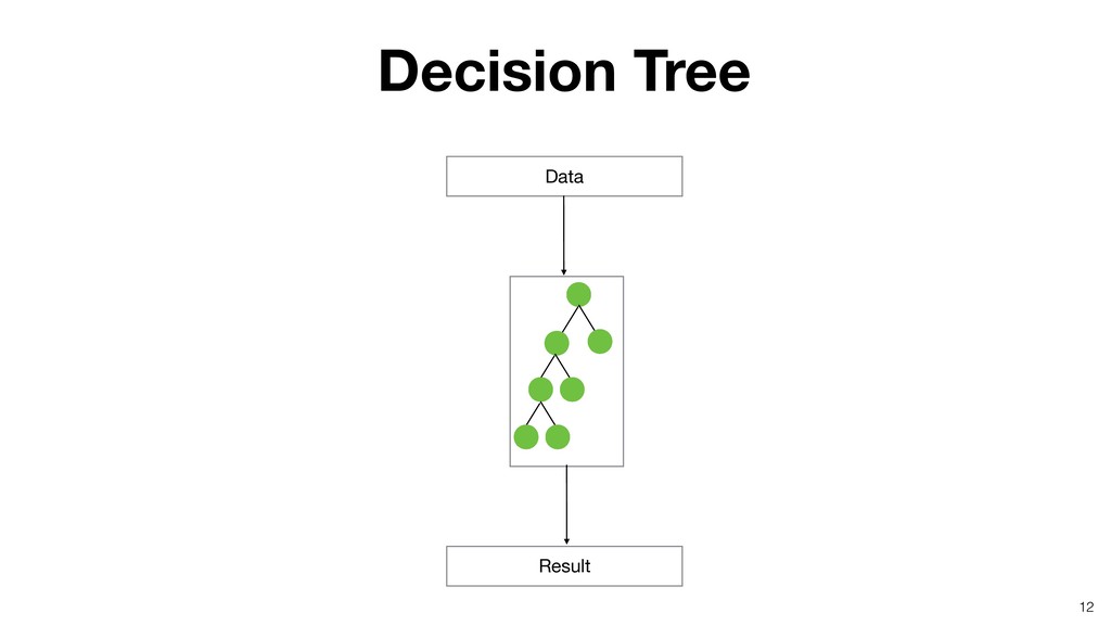
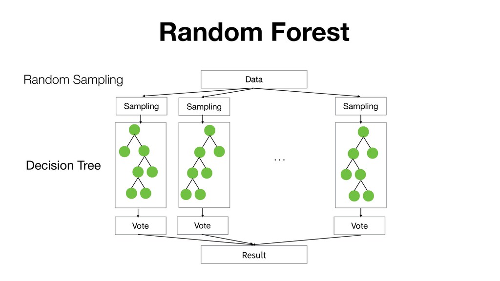
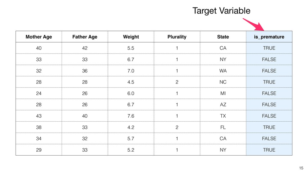
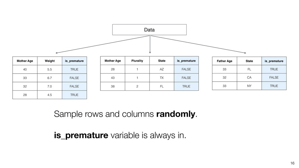
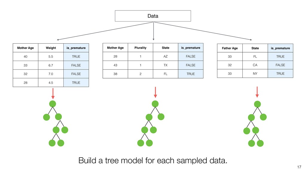
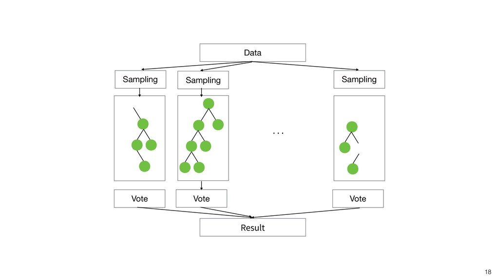
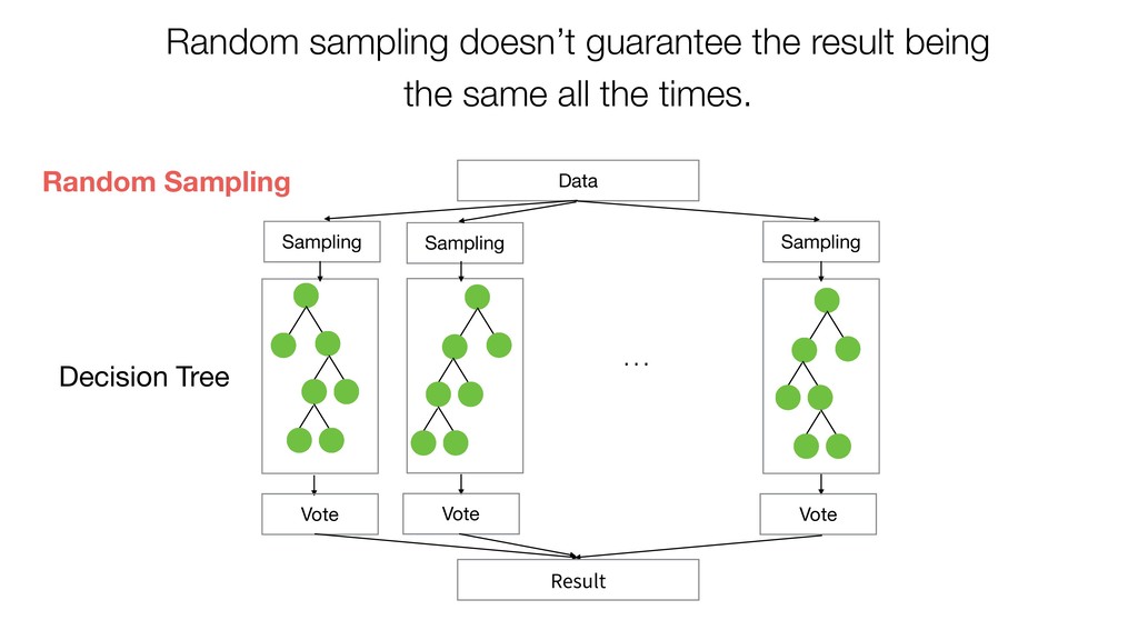
Random Forest is known as one of the ensemble machine learning algorithms that build ‘decision tree’ based models to predict either categorical or numerical outputs based on the patterns inside the data.

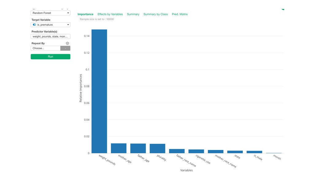
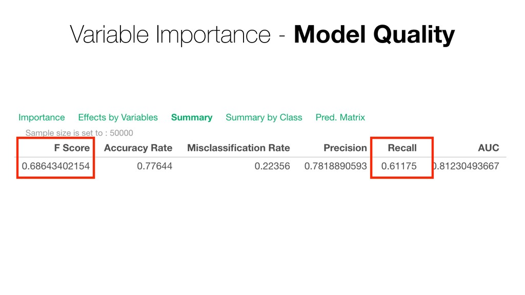
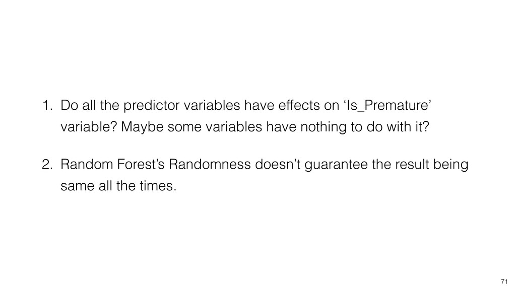
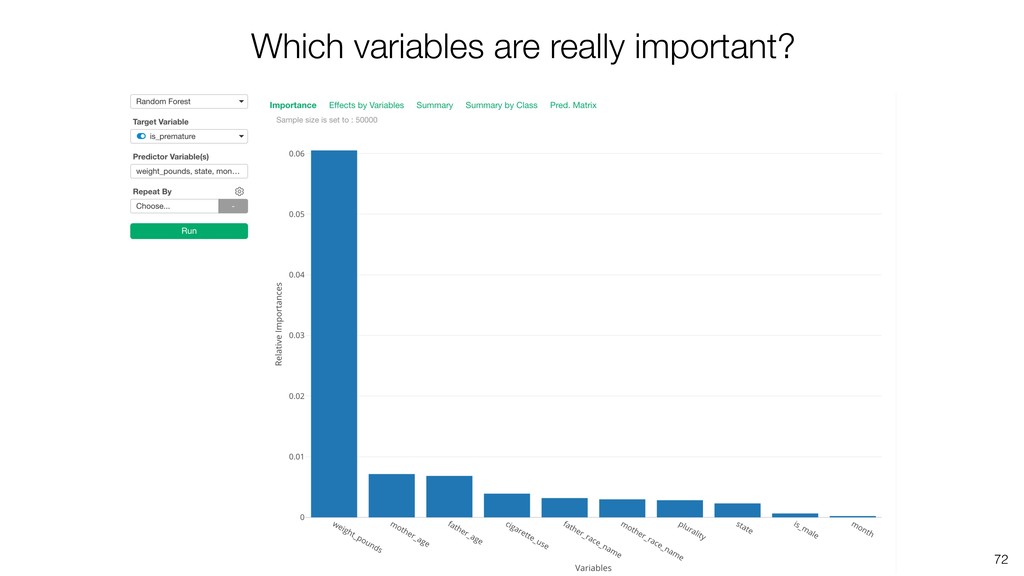
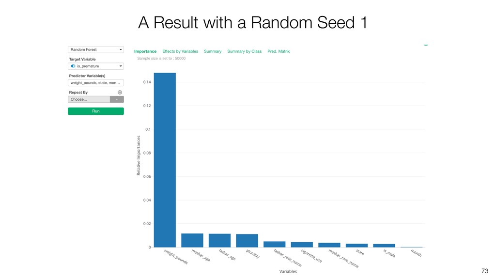
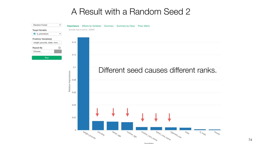
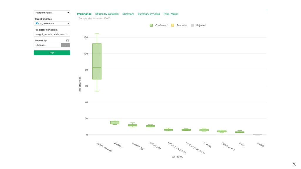
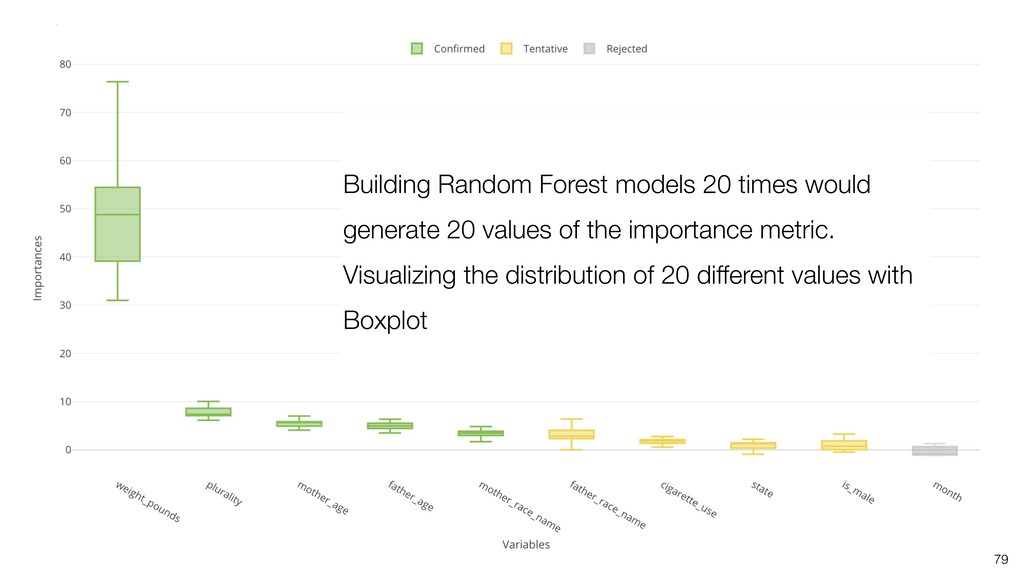
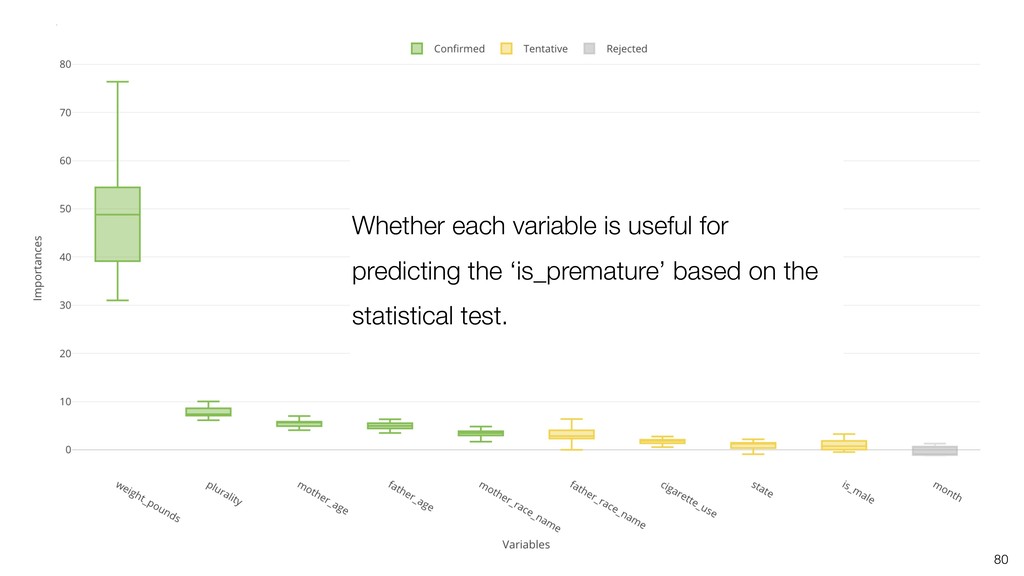
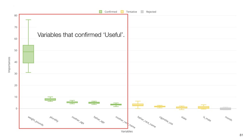
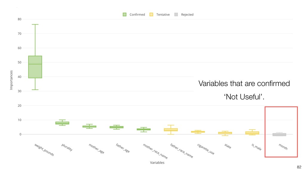
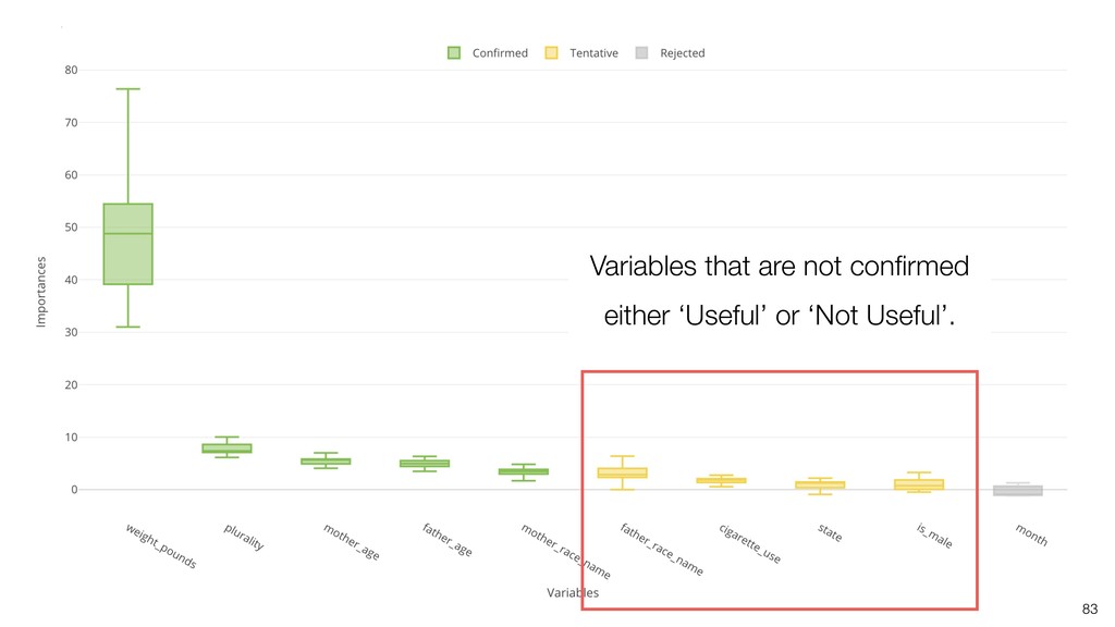
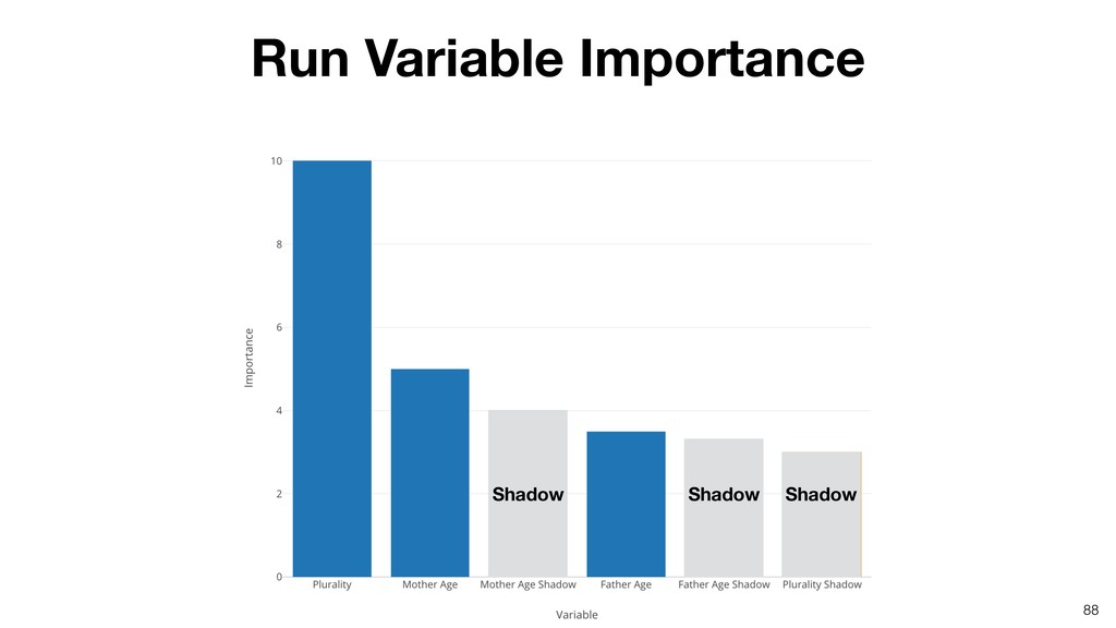
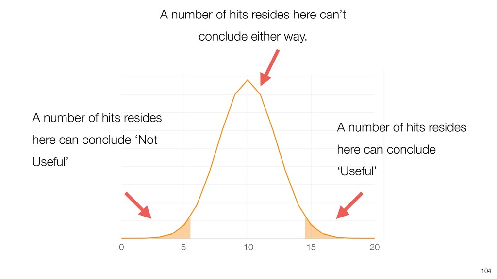
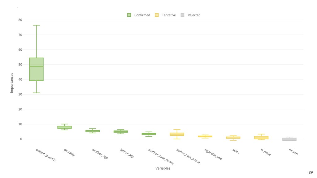
It can be often used as ‘Variable Importance’ to find which variables are more important to predict the target output.

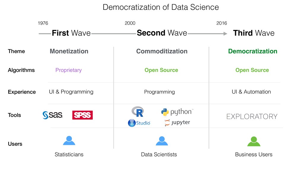
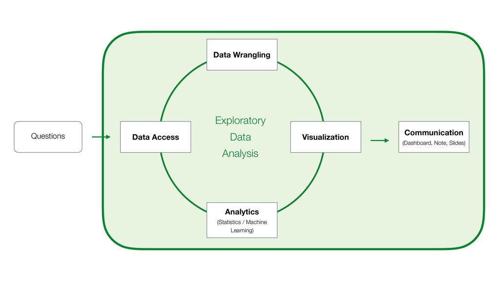
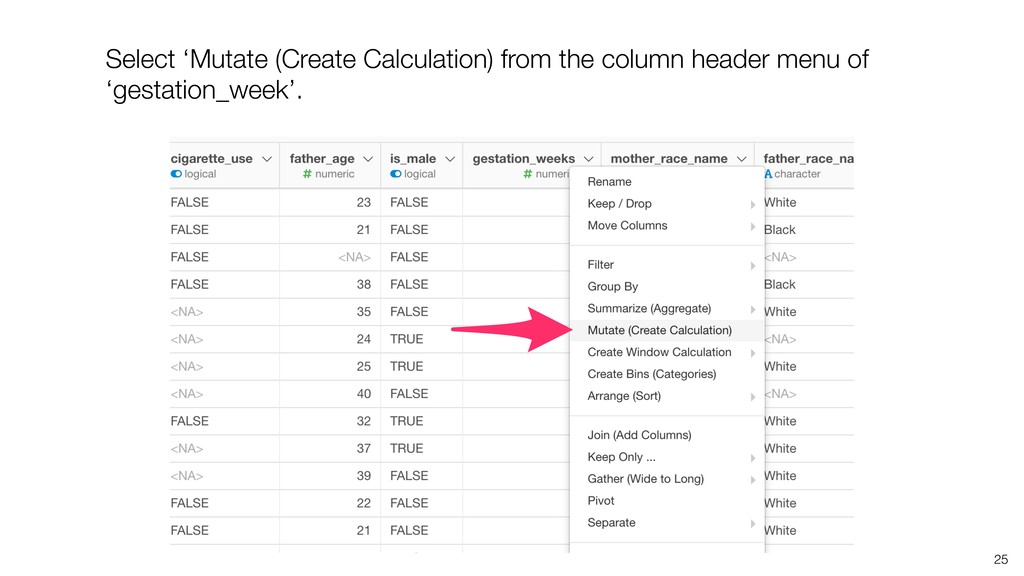
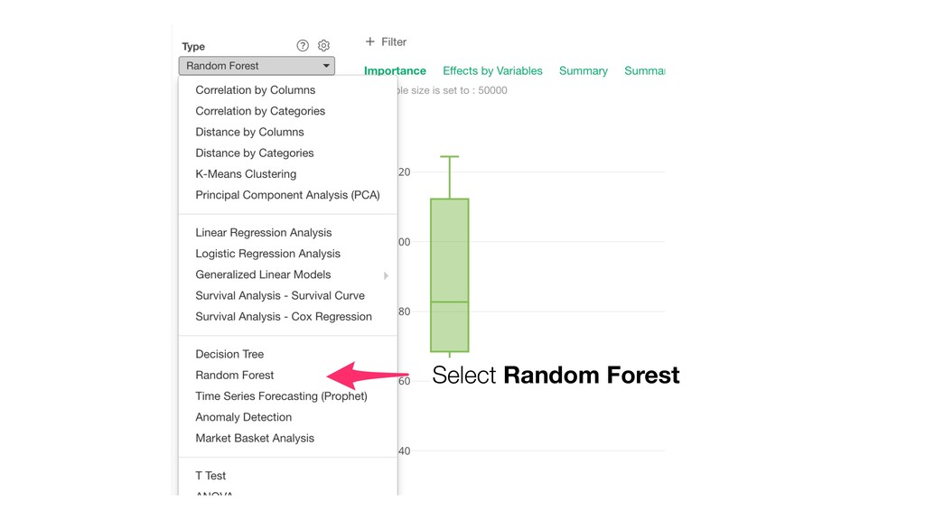
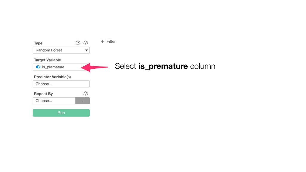
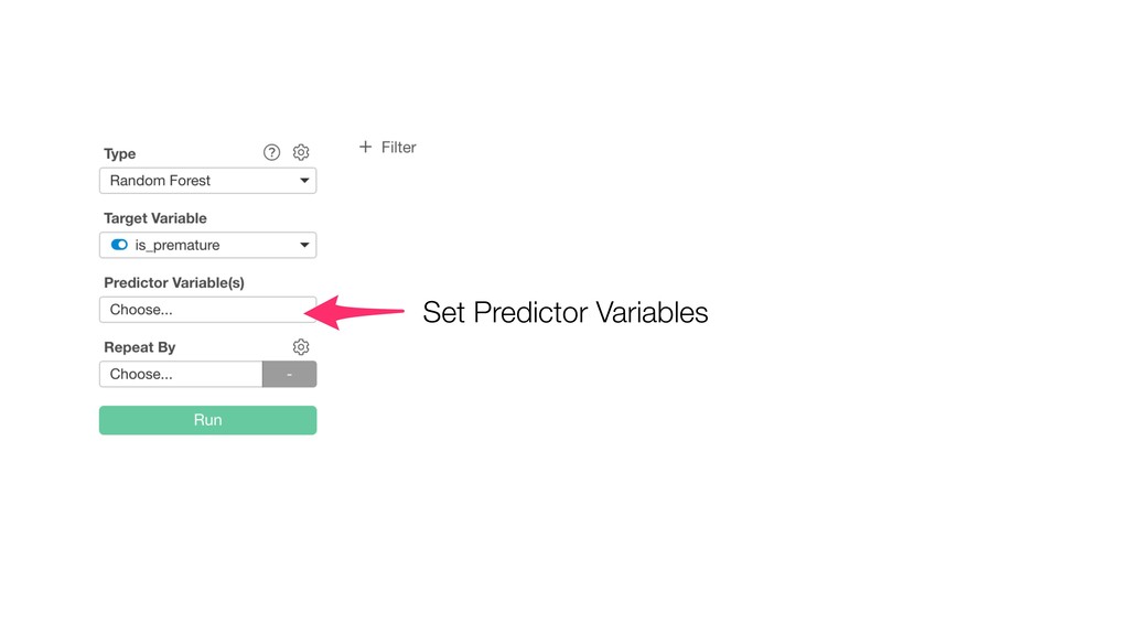
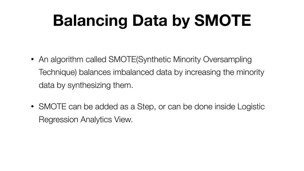
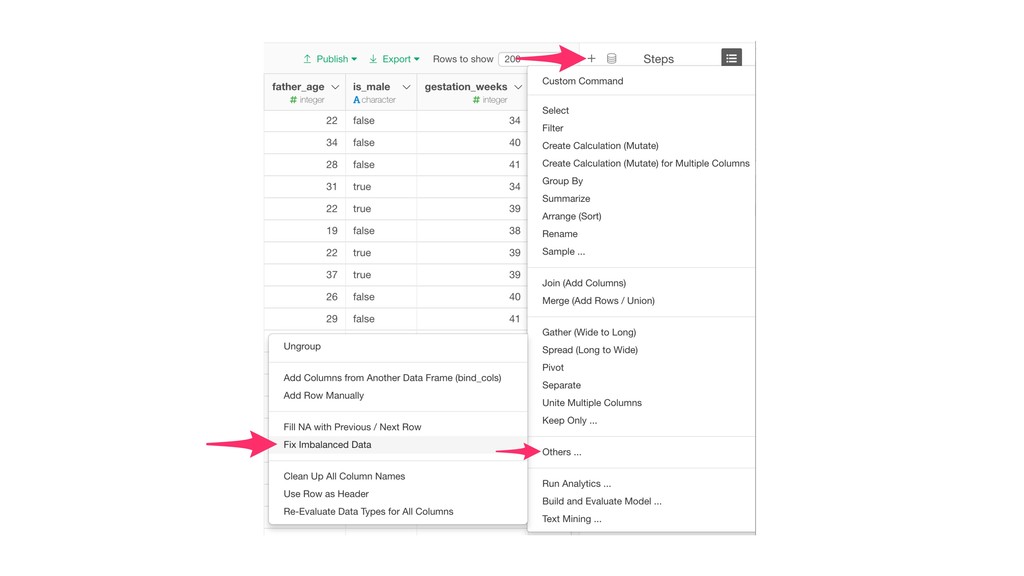
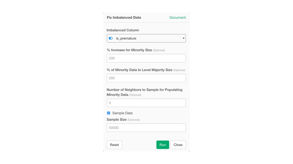
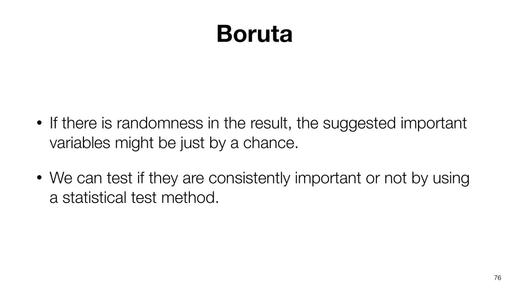
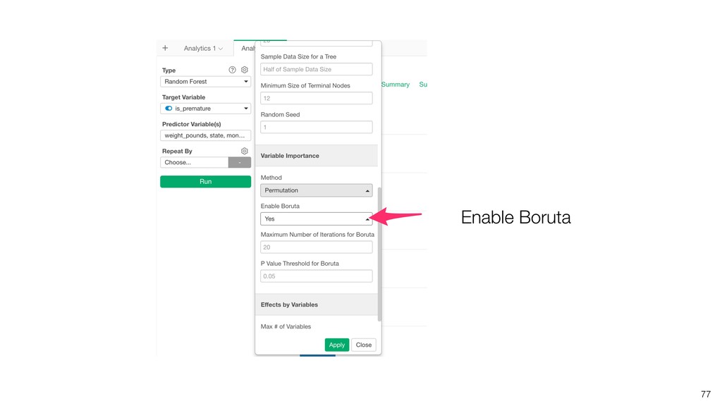
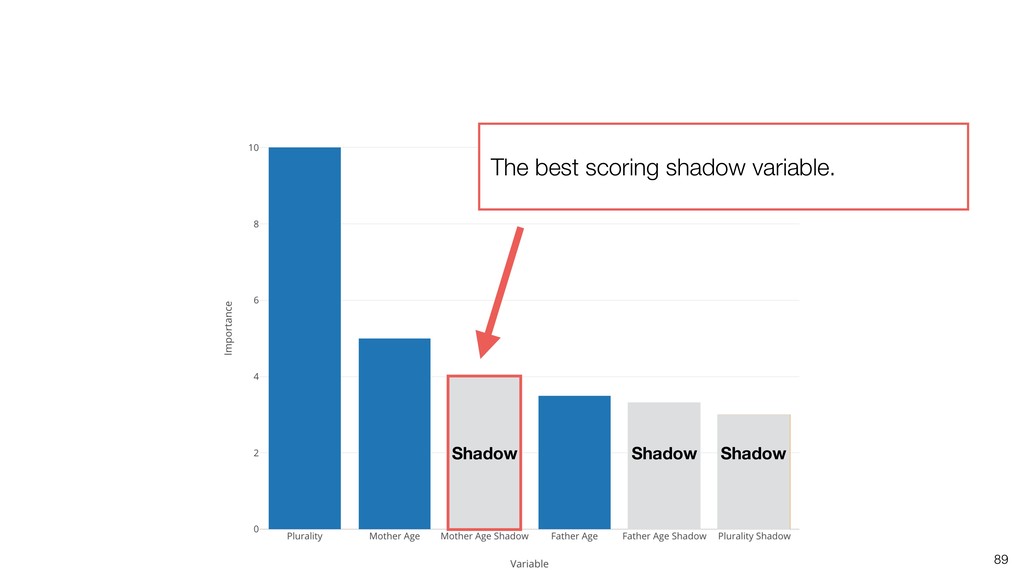
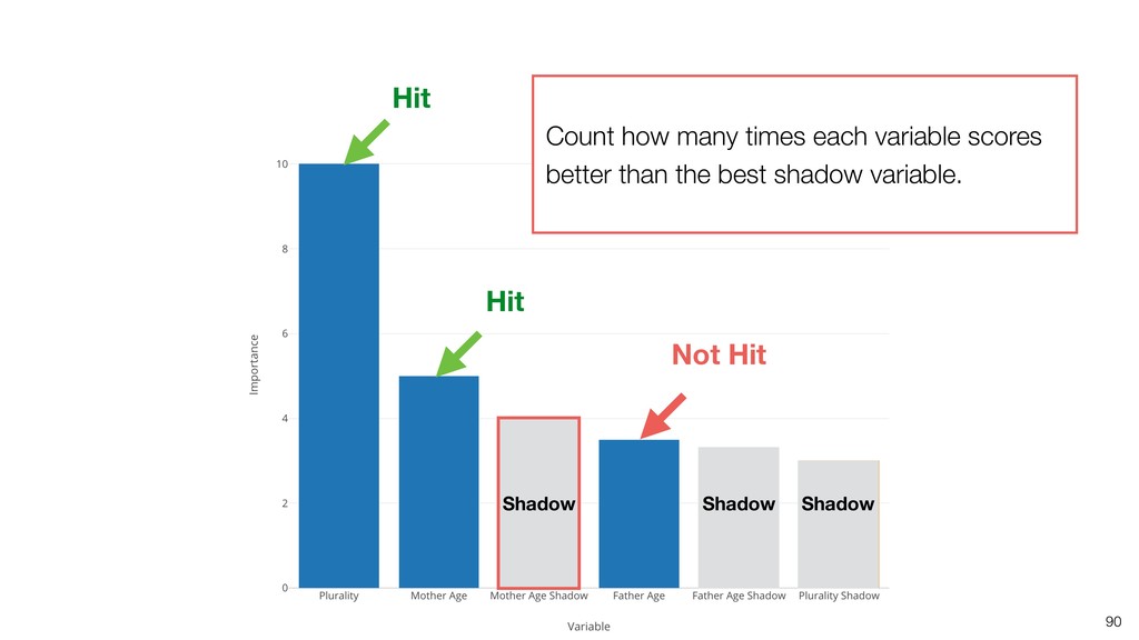
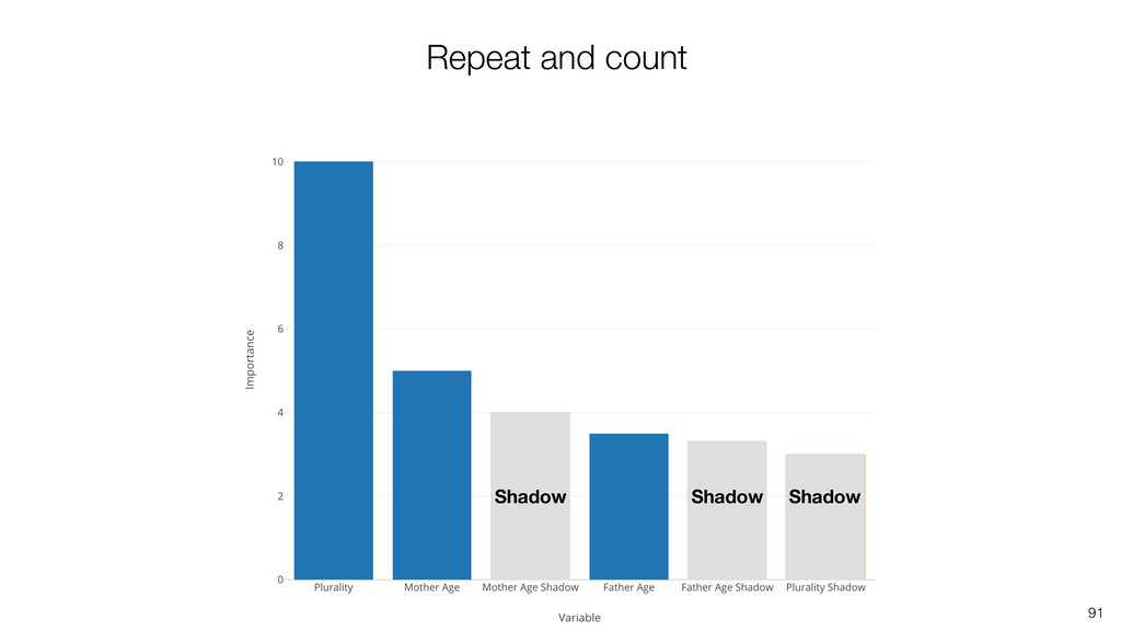
Kan will be showing how to use it with Exploratory’s Analytics view along with various methods like Boruta, EDARF, and SMOTE (adjusting imbalanced data).

Transcript

1. EXPLORATORY
2. Kan Nishida co-founder/CEO Exploratory Summary Beginning of 2016, launched Exploratory, Inc. to democratize Data Science. Prior to Exploratory, Kan was a director of development at Oracle leading development teams for building various Data Science products in areas including Machine Learning, BI, Data Visualization, Mobile Analytics, Big Data, etc. While at Oracle, Kan also provided training and consulting services to help organizations transform with data. @KanAugust Instructor
3. Mission Make Data Science Available for Everyone
4. Data Science is not just for Engineers and Statisticians. Exploratory makes it possible for Everyone to do Data Science. The Third Wave
5. First Wave Second Wave Third Wave Proprietary Open Source UI & Programming Programming 2016 2000 1976 Monetization Commoditization Democratization Statisticians Data Scientists Democratization of Data Science Algorithms Experience Tools Open Source UI & Automation Business Users Theme Users
6. Analytics Random Forest
7. Questions Communication (Dashboard, Note, Slides) Data Access Data Wrangling Visualization Analytics (Statistics / Machine Learning) Exploratory Data Analysis
8. Agenda • Random Forest 101 • Metrics of Prediction Model • Type 1 Error vs. Type 2 Error • Adjust Imbalanced Data with SMOTE • Variable Importance with Boruta
9. 9 Analytics Random Forest
10. 10 Forest
11. Ensemble Learning • Independently train multiple models • Combine the prediction from the multiple models to
 come up with the unified prediction. • Example: Random Forest, XGBoost
12. 12 Data Result Decision Tree
13. Decision Tree Random Forest Data Sampling Sampling Sampling Vote Vote Vote Result … Random Sampling
14. 14 Mother Age Father Age Weight Plurality State Is Premature 40 42 5.5 1 CA TRUE 33 33 6.7 1 NY FALSE 32 36 7.0 1 WA FALSE 28 28 4.5 2 NC TRUE 24 26 6.0 1 MI FALSE 28 26 6.7 1 AZ FALSE 43 40 7.6 1 TX FALSE 38 33 4.2 2 FL TRUE 34 32 5.7 1 CA FALSE 29 33 5.2 1 NY TRUE Data
15. 15 Mother Age Father Age Weight Plurality State is_premature 40 42 5.5 1 CA TRUE 33 33 6.7 1 NY FALSE 32 36 7.0 1 WA FALSE 28 28 4.5 2 NC TRUE 24 26 6.0 1 MI FALSE 28 26 6.7 1 AZ FALSE 43 40 7.6 1 TX FALSE 38 33 4.2 2 FL TRUE 34 32 5.7 1 CA FALSE 29 33 5.2 1 NY TRUE Target Variable
16. 16 Mother Age Weight is_premature 40 5.5 TRUE 33 6.7 FALSE 32 7.0 FALSE 28 4.5 TRUE Data Sample rows and columns randomly. is_premature variable is always in. Mother Age Plurality State is_premature 28 1 AZ FALSE 43 1 TX FALSE 38 2 FL TRUE Father Age State is_premature 33 FL TRUE 32 CA FALSE 33 NY TRUE
17. 17 Mother Age Weight is_premature 40 5.5 TRUE 33 6.7 FALSE 32 7.0 FALSE 28 4.5 TRUE Mother Age Plurality State is_premature 28 1 AZ FALSE 43 1 TX FALSE 38 2 FL TRUE Father Age State is_premature 33 FL TRUE 32 CA FALSE 33 NY TRUE Data Build a tree model for each sampled data.
18. 18 Data Sampling Sampling Sampling Vote Vote Vote Result …
19. 19 Variable Importance
20. • A model built by Random Forest can give which variables have more influence on the target variable based on Gini Impurity information. • It can be very useful at Exploratory Data Analysis phase to understand the relationships among the variables. • Random Forest is often used to extract this information, not just for prediction. Variable Importance
21. 21 Which variables might be associated with whether babies are born prematurely?
22. 22 Analytics Let’s try Random Forest!
23. Exploratory - Analytics View
24. Create a ‘is_premature’ Column 24 gestation_weeks < 37
25. Select ‘Mutate (Create Calculation) from the column header menu of ‘gestation_week’. 25
27. Select Random Forest
28. Select is_premature column
29. Set Predictor Variables
30. Select all columns except for gestation_weeks (Same info as is_premature)
32. Effects by Variable
33. How can we trust this model?
34. • Prediction Matrix a.k.a. Confusion Matrix • What are the percentage of the predicted outputs being right or wrong? • Model Summary with Metrics • Accuracy Rate, AUC, F Score, Precision, Recall, etc. Evaluate Model Quality
35. Prediction Matrix (Confusion Matrix)
36. Model Summary with Metrics
37. Prediction Matrix
38. TRUE FALSE TRUE 5 15 FALSE 15 195 Prediction Actual
39. TRUE FALSE TRUE True Positive False Negative FALSE False Positive True Negative Prediction Actual
40. TRUE FALSE TRUE True Positive False Negative FALSE False Positive True Negative Prediction Actual Accuracy Rate Accuracy Rate = (True Positive + True Negative) / Total
41. TRUE FALSE TRUE 5 15 FALSE 15 195 Prediction Actual Accuracy Rate Accuracy Rate = (5 + 195) / 240 = 0.875
42. Is Accuracy Rate Alone Good Enough?
43. TRUE FALSE TRUE True Positive False Negative FALSE False Positive True Negative Prediction Actual Type 1 Error vs. Type 2 Error Type 1 Error Type 2 Error
45. TRUE FALSE TRUE 5 15 FALSE 15 200 Prediction Actual Precision You said TRUE, but the chance of being right is only 25% (5 / (5+15)). Precision = 5 / (5+15) = 25%
46. When you predicted TRUE, it’s better be TRUE Type 1 Error
47. When you predicted TRUE, it’s better be TRUE Hi Grandma <grandma_nishida@gmail.com> Hello Kan Where are you? Are you doing ok? I’ve been worried about you since I haven’t heard back from you for a long time. Hope nothing happened to you. Please call me back. Love, Your grandma Spam Type 1 Error
48. TRUE FALSE TRUE 5 15 FALSE 15 200 Prediction Actual Recall The answer is TRUE, but the chance you can predict it is only 25%. Recall = 5 / (5+15) = 25%
49. You’d better to predict TRUE than not. When it’s TRUE but you didn’t predict it as TRUE, it can cause serious damages. Type 2 Error
50. F Score: It should score to satisfy both Recall and Precision in a balanced way. It’s between 0 and 1, The closer to 1 is better. F Score 0.25 F Score is the harmonic mean of Recall and Precision.
51. How about this model?
52. Metrics of Model Summary
53. Low score means that Type 2 Error would happen frequently.
54. You’d better to predict TRUE than not. When it’s TRUE but you didn’t predict it as TRUE, it can cause serious damages. Type 2 Error
55. TRUE FALSE TRUE 5 15 FALSE 15 200 Prediction Actual Recall The answer is TRUE, the ratio of you can predict correctly.
56. On Prediction Matrix, we can see that model is simply almost always predicting FALSE.
57. Premature birth is much fewer than not-premature birth. Imbalanced Data
58. Problem of Imbalanced Data • On Prediction Matrix, we can see that model is simply almost always predicting FALSE. • Predicting majority case (not premature) would make overall Log Likelihood higher.
59. • When the actual values are TRUE, more cases are predicted as FALSE than TRUE. • Ratio of Type 2 Error is high.
60. • When the actual values are TRUE, more cases are predicted as FALSE than TRUE. • Ratio of Type 2 Error is high. • When there is a risk of premature birth, failing to predict it can be a serious problem.
61. Adjust Imbalanced Data
62. Balancing Data by SMOTE • An algorithm called SMOTE(Synthetic Minority Oversampling Technique) balances imbalanced data by increasing the minority data by synthesizing them. • SMOTE can be added as a Step, or can be done inside Logistic Regression Analytics View.
64. Adjust Imbalanced Data We already know the data is skewed. Let’s use “Adjust Imbalanced Data”.
65. Prediction Matrix Prediction is no longer skewed towards FALSE.
66. Variable Importance - Model Quality
67. Balancing Data by SMOTE - As a Step
70. 70 Challenges with Variable Importance
71. 1. Do all the predictor variables have effects on ‘Is_Premature’ variable? Maybe some variables have nothing to do with it? 2. Random Forest’s Randomness doesn’t guarantee the result being same all the times. 71
72. 72 Which variables are really important?
73. 73 A Result with a Random Seed 1
74. 74 Different seed causes different ranks. A Result with a Random Seed 2
75. Decision Tree Data Sampling Sampling Sampling Vote Vote Vote Result … Random Sampling Random sampling doesn’t guarantee the result being the same all the times.
76. 76 • If there is randomness in the result, the suggested important variables might be just by a chance. • We can test if they are consistently important or not by using a statistical test method. Boruta
77. 77 Enable Boruta
79. 79 Building Random Forest models 20 times would generate 20 values of the importance metric. Visualizing the distribution of 20 different values with Boxplot
80. 80 Whether each variable is useful for predicting the ‘is_premature’ based on the statistical test.
81. 81 Variables that confirmed ‘Useful’.
82. 82 Variables that are confirmed ‘Not Useful’.
83. 83 Variables that are not confirmed either ‘Useful’ or ‘Not Useful’.
84. 84 How does Boruta do the test?
85. • Count a number of times a given variable’s variable importance score is better than the shadow variables for each variable. • Perform a hypothesis test for the counts and evaluate the statistical significance for each variable.
86. 86 Plurality Mother Age Father Age 1 25 27 3 35 40 2 40 41 1 22 22 1 33 35 Data
87. 87 Plurality Mother Age Father Age 1 25 27 3 35 40 2 40 41 1 22 22 1 33 35 Create Shadow Plurality Shadow Mother Age Shadow Father Age Shadow 1 22 41 1 44 22 1 35 35 3 25 40 2 40 27 • Copy the original variables and shuffle the values randomly. • These randomly shuffled variables shouldn’t have any association with the target variables.
88. 88 Run Variable Importance Shadow Shadow Shadow
89. 89 Shadow Shadow Shadow The best scoring shadow variable.
90. 90 Hit Hit Not Hit Shadow Shadow Shadow Count how many times each variable scores better than the best shadow variable.
91. 91 Repeat and count Shadow Shadow Shadow
92. 92 Hypothesis Test Null HypothesisɿThere is no difference between a given variable and the best shadow variable in terms of the variable importance.
 Alternative Hypothesis 1 : A given variable is better than the best shadow. (Useful) Alternative Hypothesis 2 : A given variable is worse then the best shadow variable. (Not Useful)
93. 93 Under the assumption of Null Hypothesis,
 a distribution of a number of Hits for 20 experiments. 10 5 20 15 0
94. 94 If we take 5% (0.05) as a threshold of significance… 10 5 20 15 0 P Value : 5%
95. 95 10 5 20 15 0 If a given variable was better at 15 times out of 20…
96. 96 10 5 20 15 0 this can happen only with less than 5% of chance.
97. 97 10 5 20 15 0 We can reject the null hypothesis and conclude that this variable is useful for prediction.
98. 98 If a given variable was better at only 5 times out of 20… 10 5 20 15 0
99. 99 10 5 20 15 0 this can happen only with less than 5% of chance.
100. 100 10 5 20 15 0 We can reject the null hypothesis and conclude that this variable is Not Useful for prediction.
101. 101 10 5 20 15 0 If a given variable was better at 12 times out of 20…
102. 102 10 5 20 15 0 this can happen at greater than 5% of chance.
103. 103 10 5 20 15 0 We can NOT reject the null hypothesis, can NOT conclude that this variable is whether Useful or Not Useful for prediction.
104. 104 10 5 20 15 0 A number of hits resides here can conclude ‘Useful’ A number of hits resides here can’t conclude either way. A number of hits resides here can conclude ‘Not Useful’
106. Q & A
107. Contact Email kan@exploratory.io Data Science Training https://exploratory.io/training Twitter @KanAugust Online Seminar https://exploratory.io/online-seminar