Exploratory Data Analysis Part 2 - Correlation and Association

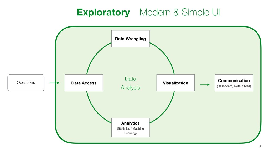
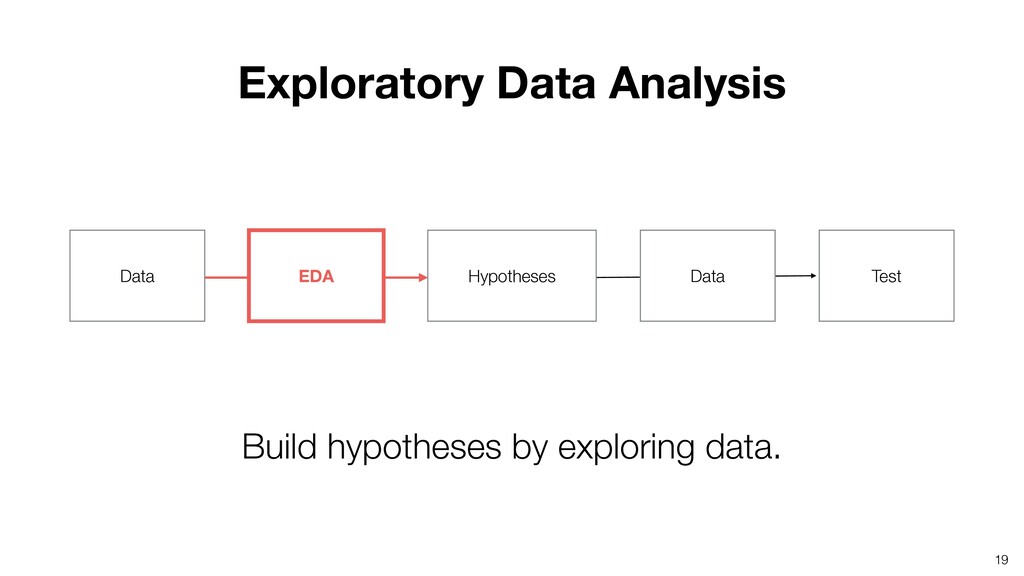
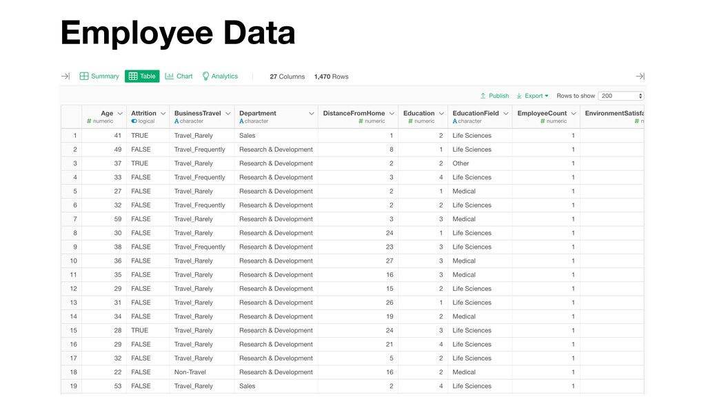
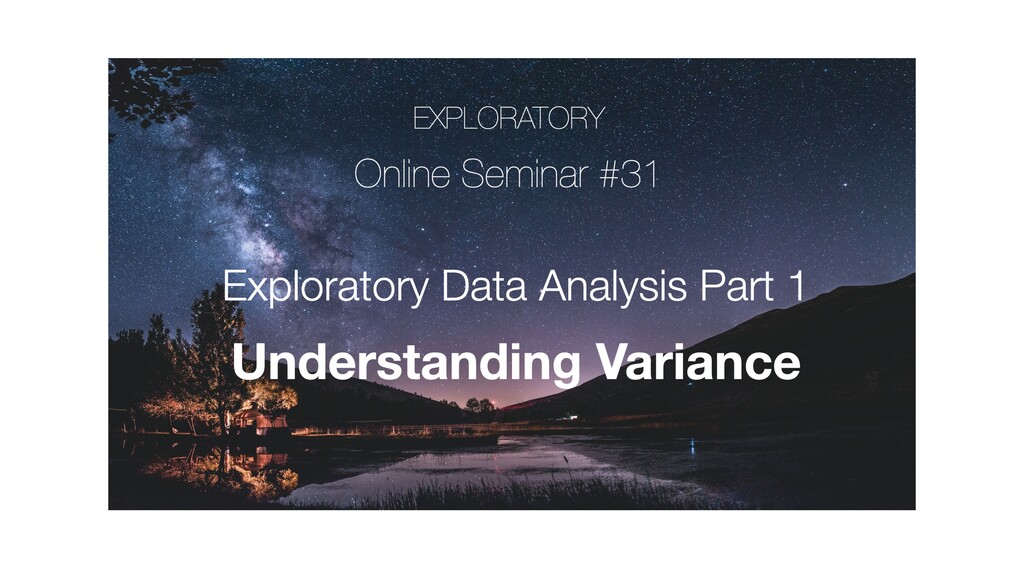
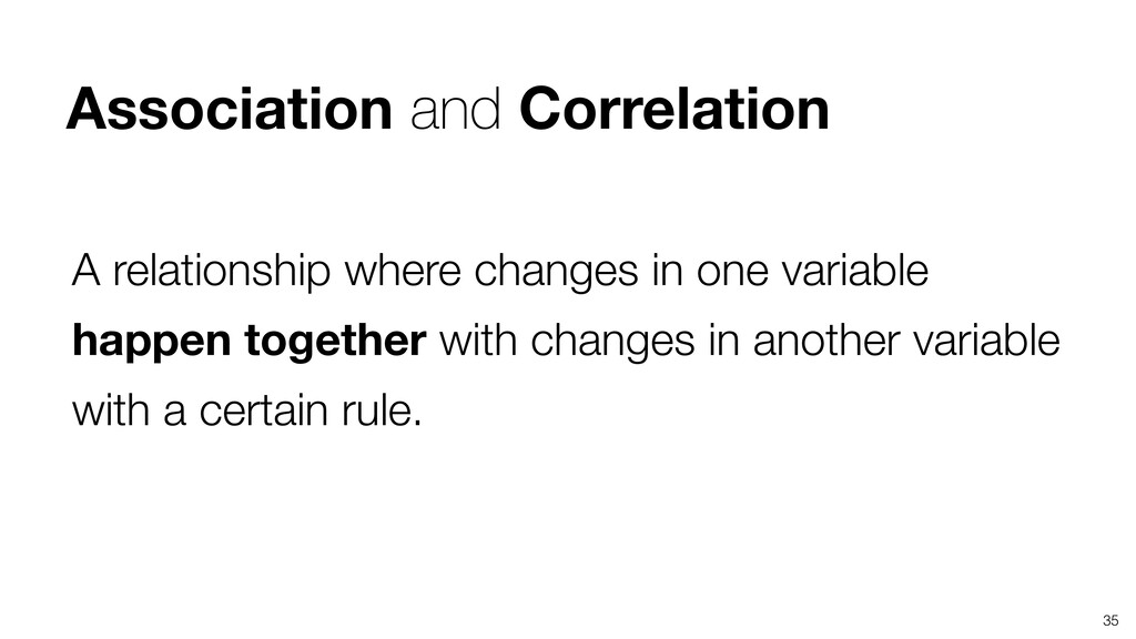
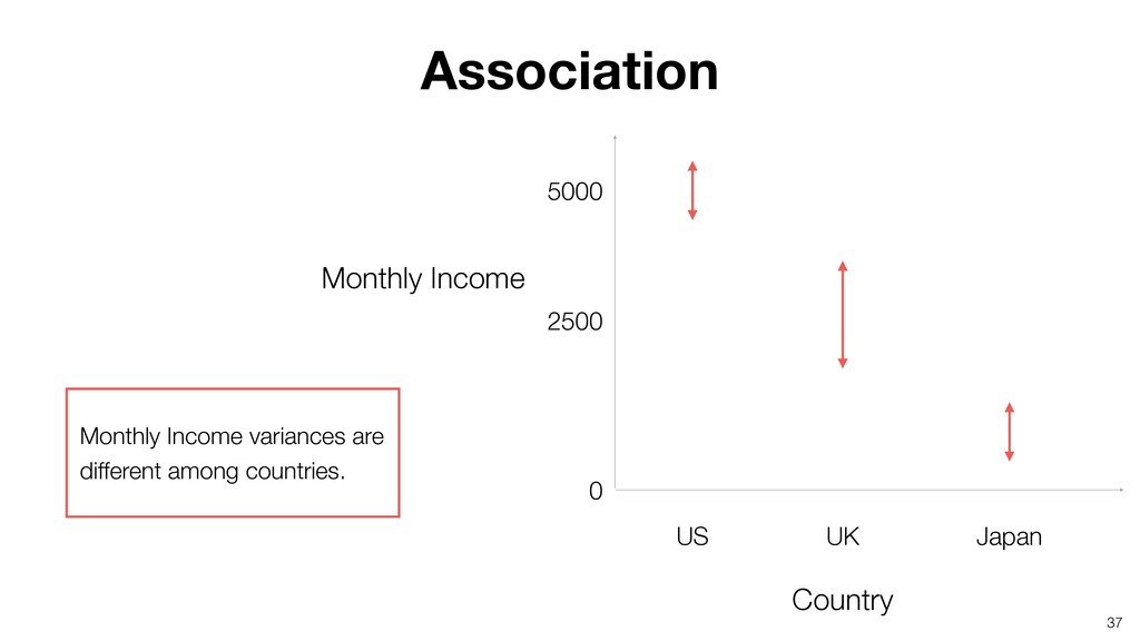
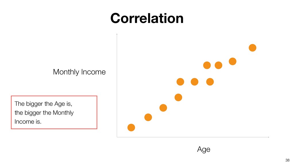
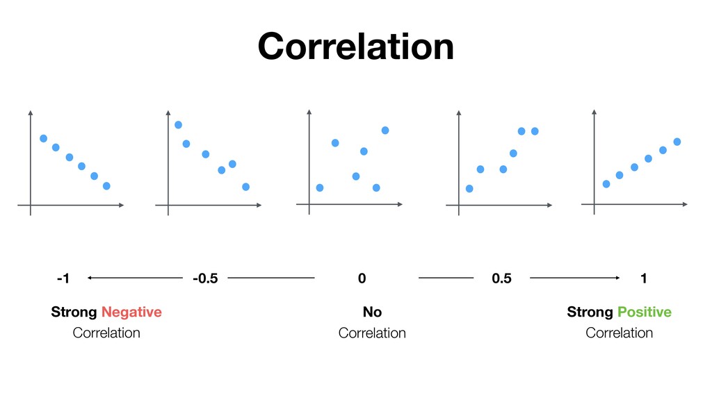
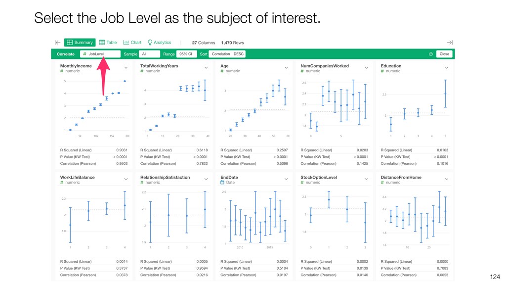
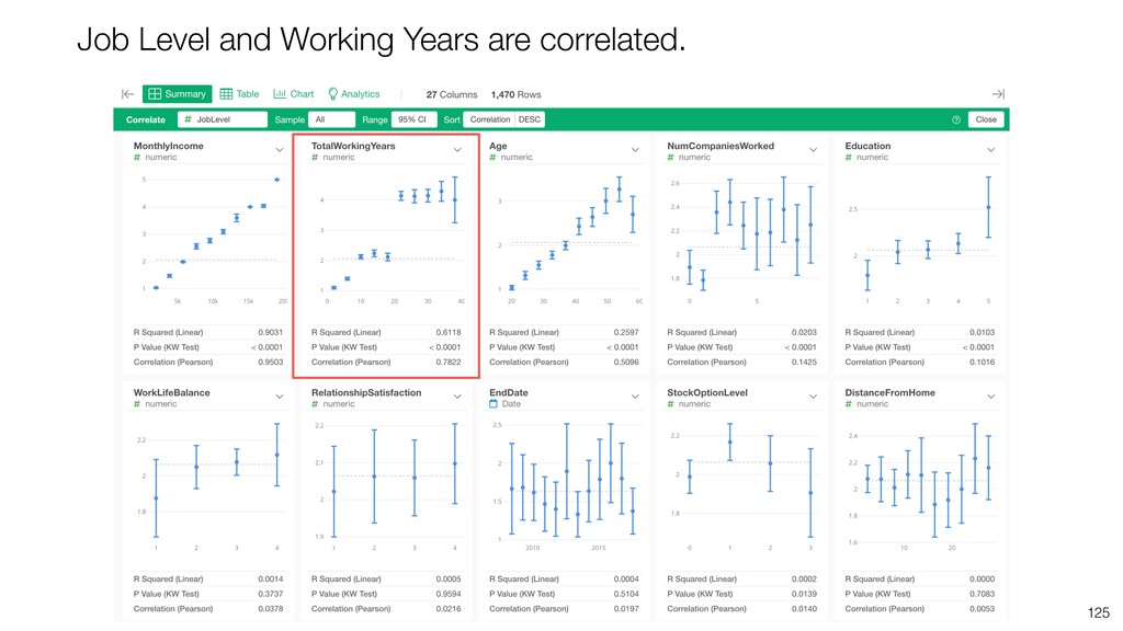
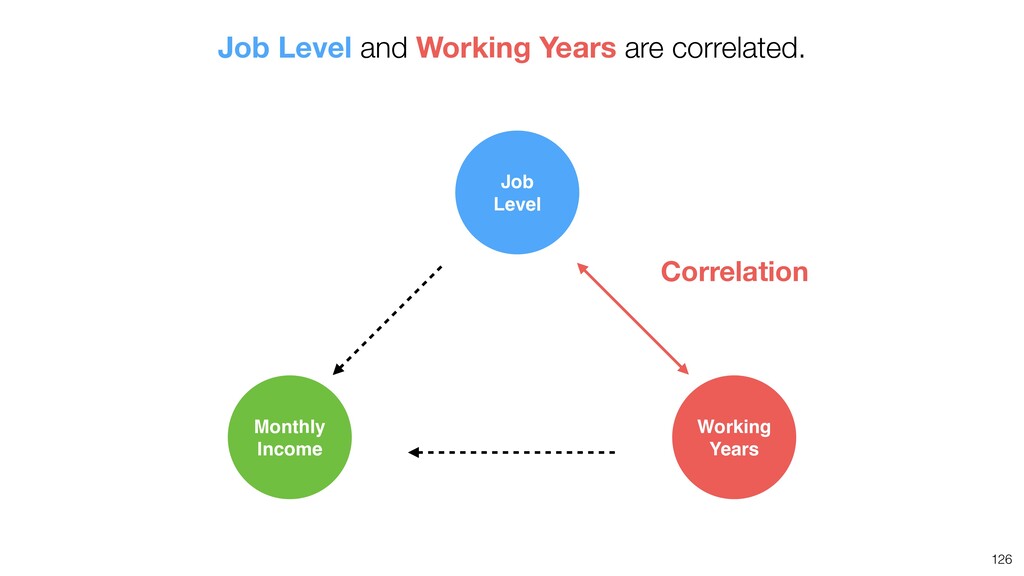
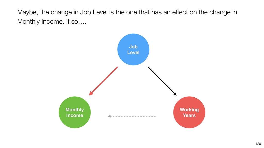
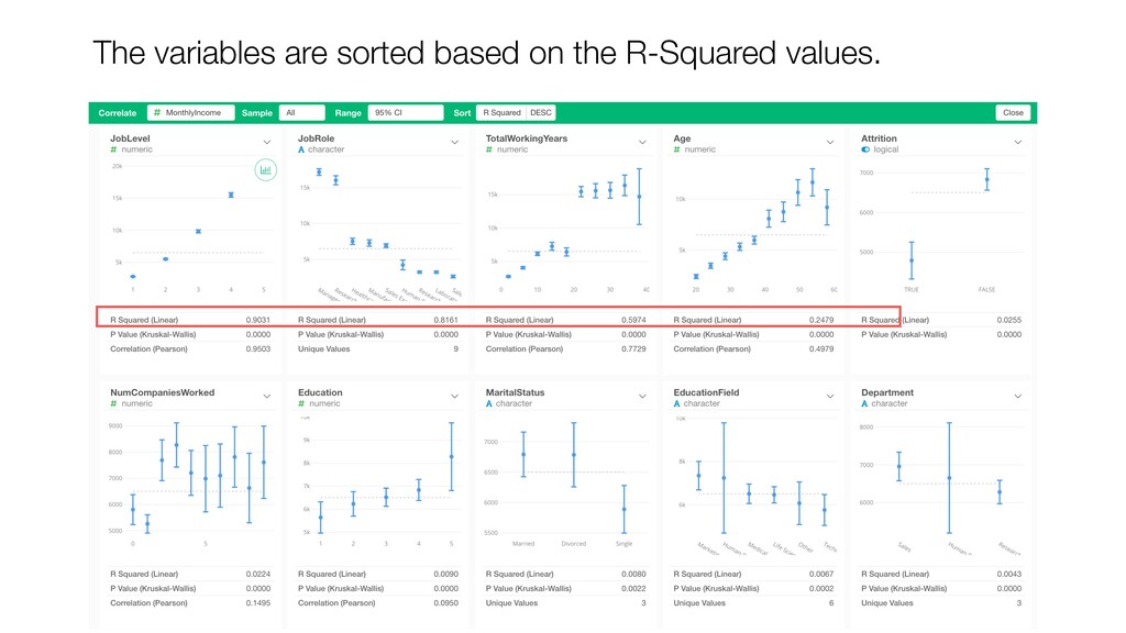
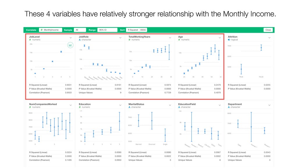
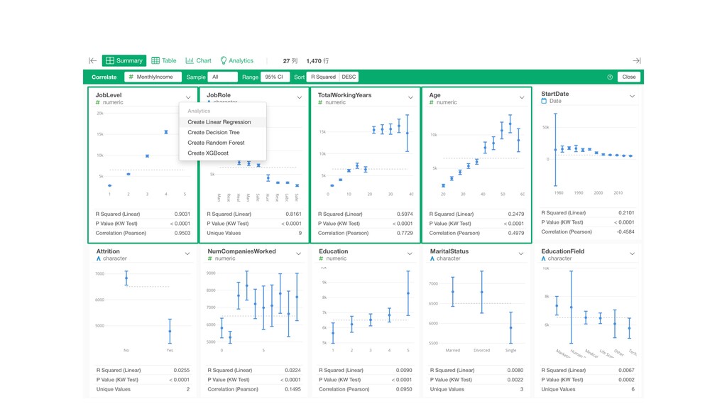
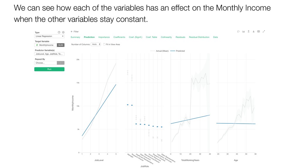
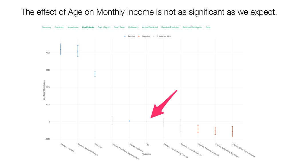
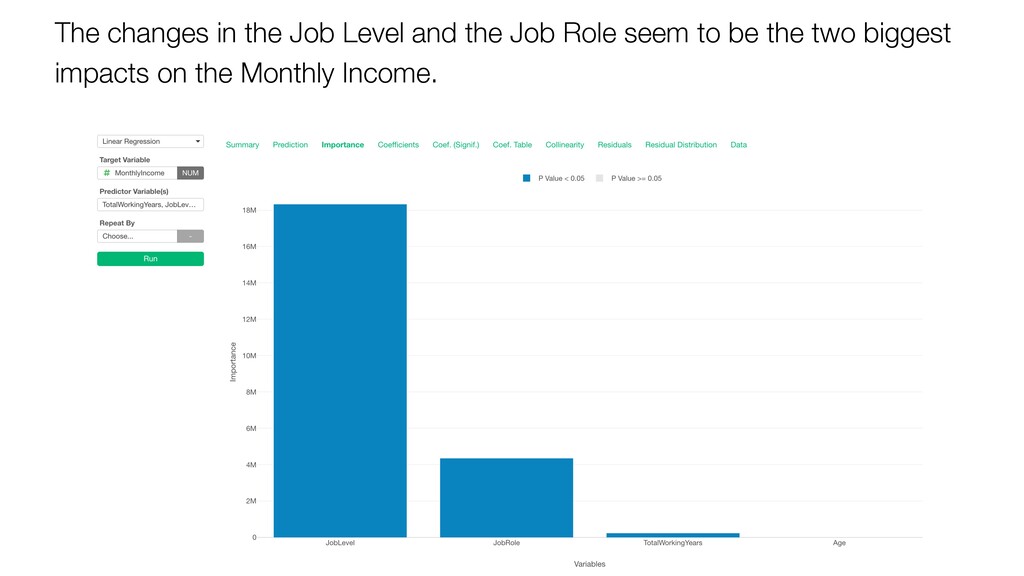
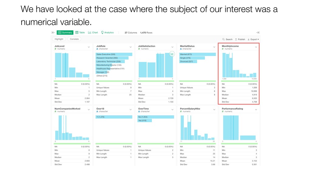
This is a part of the Exploratory Data Analysis Workshop. In this episode, we'll talk about the correlation and association between variables and introduce some effective methods to investigate such relationships.

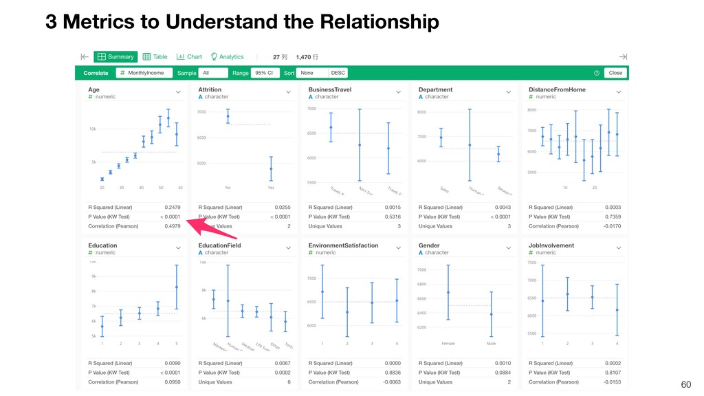
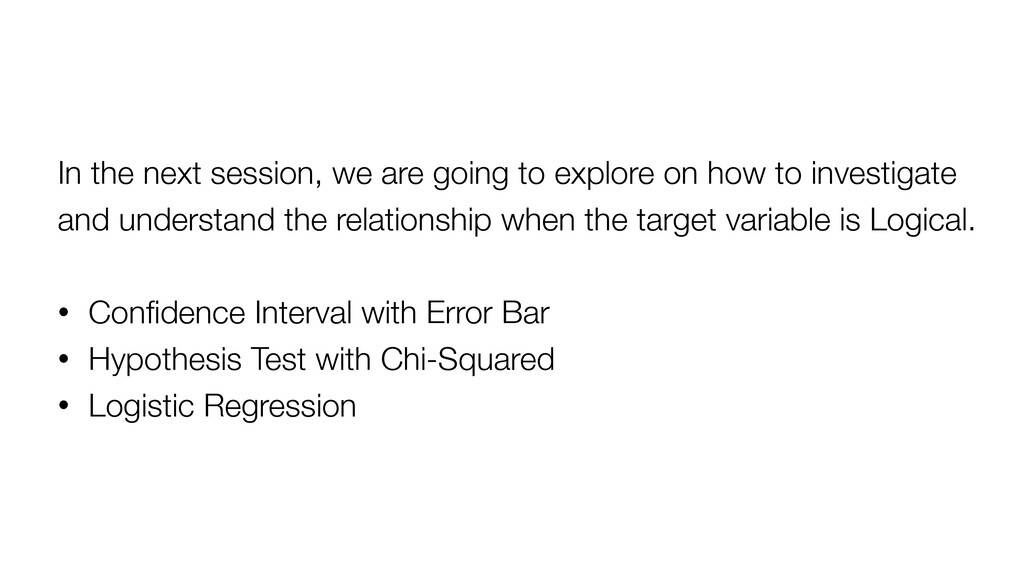
* Correlation / Association
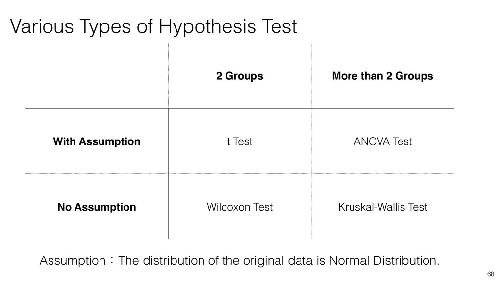
* Kruskal-Wallis Test
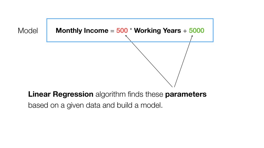
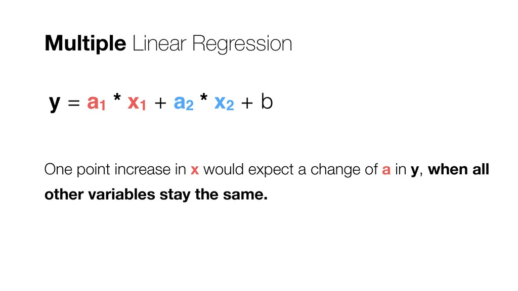
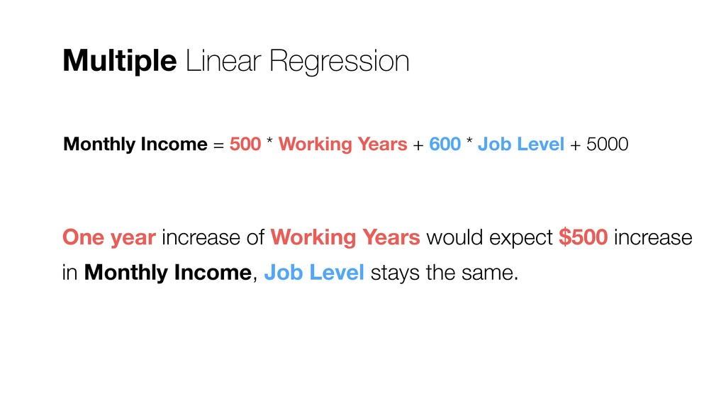
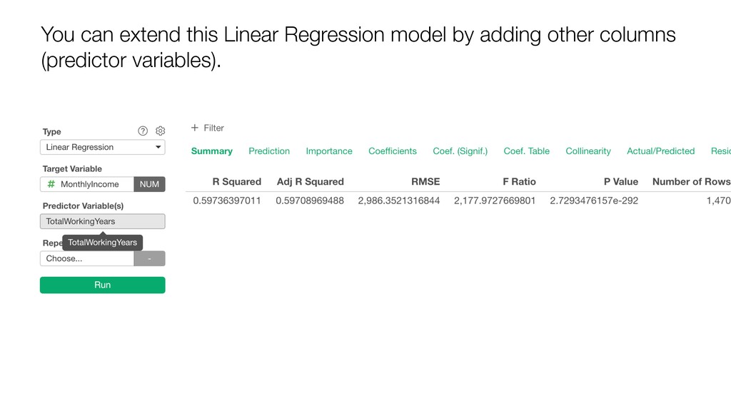
* Linear Regression

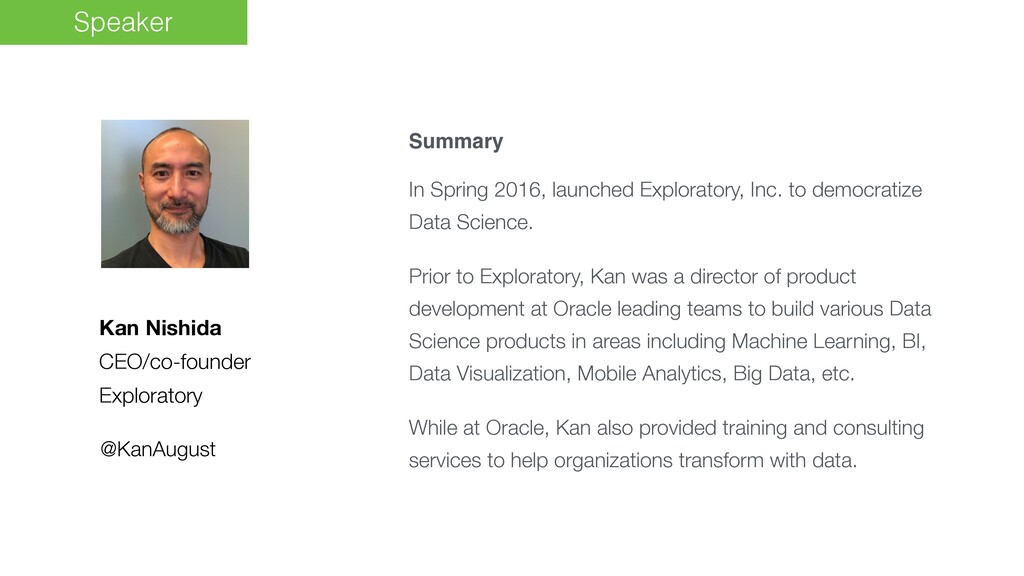
Exploratory(https://exploratory.io)

Transcript

1. EXPLORATORY Online Seminar #32 Exploratory Data Analysis Part 2 Correlation & Association
2. Kan Nishida CEO/co-founder Exploratory Summary In Spring 2016, launched Exploratory, Inc. to democratize Data Science. Prior to Exploratory, Kan was a director of product development at Oracle leading teams to build various Data Science products in areas including Machine Learning, BI, Data Visualization, Mobile Analytics, Big Data, etc. While at Oracle, Kan also provided training and consulting services to help organizations transform with data. @KanAugust Speaker
3. Mission Democratize Data Science
4. 4 Questions Communication Data Access Data Wrangling Visualization Analytics (Statistics / Machine Learning) Data Analysis Data Science Workflow
5. 5 Questions Communication (Dashboard, Note, Slides) Data Access Data Wrangling Visualization Analytics (Statistics / Machine Learning) Data Analysis ExploratoryɹModern & Simple UI
6. EXPLORATORY Online Seminar #32 Exploratory Data Analysis Part 2 Correlation & Association
7. 7 Wayne Gretzky
8. 8 - Wayne Gretzky “I skate to where the puck is going to be, not where it has been.”
9. 9 Predict how many customers we will have. Prediction e.g. Customers will be 1000 by end of this year.
10. 10 - Kan Nishida “I control where the puck is going to be, not the puck controls where I should be.”
11. 11 e.g. We want to grow Customers to 1000. What can we do to make that happen? Control
12. 12 Hypothesis If the weather will be warm, we will have more customers. If we offer 10% discount, we would have more customers. Prediction Control
13. 13 Test Hypotheses by Experimenting and Collecting Data • Hypothesis Test • A/B Test Hypotheses Data Test Discount increases more customers
14. 14 Test Hypotheses by Experimenting and Collecting Data • Hypothesis Test • A/B Test Hypotheses Data Test Discount increases more customers Confirmatory Analysis
15. 15 Hypotheses Data Test How can we build Hypothesis?
16. 16 Intuition! Hypotheses Data Test
17. 17 Build Hypothesis based on Data Hypotheses Data Test Data How about Data?
18. 18 John Tukey built the method and published a book called ‘Exploratory Data Analysis’ in 1970s.
19. 19 Build hypotheses by exploring data. EDA Hypotheses Data Test Data Exploratory Data Analysis
20. An exploratory and iterative process of asking many questions and find answers from data in order to build better hypothesis for Explanation, Prediction, and Control. 20 Exploratory Data Analysis (EDA)
21. An exploratory and iterative process of asking many questions and find answers from data in order to build better hypothesis for Prediction and Control. 21 Exploratory Data Analysis (EDA)
22. 22 • How the variation in variables? • How are the variables associated (or correlated) to one another? Two Principle Questions for EDA
23. Employee Data
24. Want to understand how the salary is decided.
25. 25 Employee Salary $6,503 Average
26. 26 Data varies…
31. The variance is an opportunity for Data Analysis. 31
32. 32 If there is no variance…
33. 33 Variance is a good starting point for building hypothesis of association or causal relationship. If there is variance, we can ask “What makes the variance?” and start investigating further. ʁ Income
34. What makes Monthly Income different? 34
35. 35 A relationship where changes in one variable happen together with changes in another variable with a certain rule. Association and Correlation
36. 36 Association Correlation Any type of relationship between two variables. A certain type of (usually linear) association between two variables
37. 37 US UK Japan 5000 2500 Monthly Income variances are different among countries. Country Monthly Income 0 Association
38. 38 Age Monthly Income The bigger the Age is, the bigger the Monthly Income is. Correlation
39. Strong Negative Correlation No Correlation Strong Positive Correlation 0 1 -1 -0.5 0.5 Correlation
40. 40 0 30 20 If we can find a correlation between Monthly Income and Working Years… 10 $20,000 $1,000 Working Years Monthly Income
41. 41 0 30 20 10 $20,000 $1,000 Working Years If Working Years is 20 years, Monthly Income would be around $15,000. $15,000 Monthly Income
42. 42 ʁ Income If we can find strong correlations, it makes it easier to explain how Monthly Income changes and to predict what Monthly Income will be.
43. Correlation is not equal to Causation. Causation is a special type of Correlation. If we can confirm a given Correlation is Causation, then we can control the outcome. Warning!
44. What makes the Monthly Income increase or decrease?
45. 45 Click on ‘Correlation’ button to open the Correlation Mode.
46. 46 Select ‘Monthly Income’ column as a subject of our interest.
47. 47 Each variable shows its relationship with Monthly Income.
48. For numerical variables, it divides into 10 sections and shows the mean and the 95% confidence interval for each section. 48
49. You can select from various range types.
50. What is Confidence Interval?
51. 51 True Meanɿ$5,000 Mean of this dataɿ$5,200
52. 52 We don’t really know True mean. True Meanɿ? Mean of this dataɿ$5,200
53. 5,200 5,000 True Mean Mean of this data 53 We don’t know True mean of the Monthly Income. We might be missing some employees, some employees data is not accurate, the timing is not right, there is some bias, etc. But, we know the mean of this data in our hands.
54. 5,200 5,000 54 Can we have a range of this mean value so that we can say that True mean should reside somewhere within this range? 95% Confidence Interval
55. 55 If we take many samples from the population data and calculate the 95% confidence interval of each mean…
56. 56 True Mean 95% of all the confidence intervals should include the True mean. }Sample
57. 57 We happen to be looking at one of the mean and the 95% confidence interval. }αϯϓϧ True Mean
60. 60 3 Metrics to Understand the Relationship
61. Strong Negative Correlation No Correlation Strong Positive Correlation 0 1 -1 -0.5 0.5 Correlation
62. 62 Select ‘Correlation’ to sort the variables based on the correlation values.
63. 63 The variables are sorted based on the Correlation values.
64. 64 Monthly Income Job Level Monthly Income and Job Role are correlated for some degrees.
65. 65 Are these relationships significant?
66. 66 Hypothesis Test
67. This significance test is based on the Kruskal-Wallis test, which is used to test if the differences in the variance among variables are significant, with no assumption of normality in the target variable. Kruskal-Wallis Test
68. 2 Groups More than 2 Groups With Assumption t Test ANOVA Test No Assumption Wilcoxon Test Kruskal-Wallis Test AssumptionɿThe distribution of the original data is Normal Distribution. Various Types of Hypothesis Test 68
69. It indicates the probability of observing the relationship between the Monthly Income and the Job Level by chance when assuming that there is no relationship between them. It shows less than 0.0001, which means that the chance of observing the relationship we see here is very minimal. And this means that the above assumption doesn’t seem to be working. Therefore, we can conclude that Monthly Income and Job Level indeed have some degree of relationship. P-Value
70. 70 To visualize the relationship, click ‘Scatter Chart’ from the column header menu.
71. 71 The relationship between Monthly Income and Job Level is visualized with a Scatter plot chart.
72. 72 We can check the same metrics information.
73. 73 By the way, Job Level is rather Categorical than Numerical.
74. 74 Boxplot is better to visualize the relationship between Numerical and Categorical variables.
75. 75 Select ‘As Number’ to change the X-Axis scale.
76. Investigate Correlation with Linear Regression Model
77. You can create a Linear Regression model to investigate the relationship between Monthly Income and Job Level further.
78. The first thing you see is a tab called ‘Prediction’ where you can see the predicted values of Monthly Income based on the Job Level.
79. The gray line shows the mean (average) at each numeric value of Job Level (e.g. 1, 2, 3…) and the blue line is the predicted values by the Linear Regression Model.
80. Linear Regression Basics 80
81. 81 Monthly Income 5000 10000 15000 25000 20000 Working Years 40 20 10 0 30
82. Want to find a simple pattern that can explain both the given data and the data we don’t have at hands. 82
83. 83 Draw a line to make the distance between the actual values and the line to be minimal. 40 20 10 0 30 5000 10000 15000 25000 20000
84. 84 40 20 10 0 30 5000 10000 15000 25000 20000 Monthly Income = 500 * Working Years + 5000
85. 85 5000 Slopeɿ500 40 20 10 0 30 Monthly Income = 500 * Working Years + 5000
86. 86 5000 40 20 10 0 30 Y Intercept Monthly Income = 500 * Working Years + 5000
87. Linear Regression algorithm finds these parameters based on a given data and build a model. Model Monthly Income = 500 * Working Years + 5000
88. Target value (y) can be estimated from a single variable (x) y = a * x + b Simple Linear Regression Monthly Income = 500 * Working Years + 5000
89. MonthlyIncome = 4041 * Job Level -1839
90. The model with Job Level and Working Years is now showing the R Squared as 0.90.
91. R Squared • How good does the model perform compared to a null model? • How can a given variable(s) explain the variance of the target variable. • It can be between 0 and 1, 1 being the highest. • Square of the Correlation
92. When R Squared is high… When R Squared is low… Let's take a look at High and Low scenarios.
93. When R Squared is close to 1. 93
94. 94 Mean Prediction 55K 60K 65K 0 70K 75K 80K 85K 50K Monthly Income Working Years
95. 95 Let’s look at this data 55K 60K 65K 70K 75K 80K 85K 0 50K Mean Prediction Monthly Income Working Years
96. 96 55K 60K 65K 70K 75K 80K 85K 0 50K Mean Prediction Monthly Income Working Years
97. The variance that is not explained by this model. 97 ࣮ଌ 55K 60K 65K 70K 75K 80K 85K 0 The variance that is explained by this model. 50K Mean Prediction Monthly Income Working Years
98. 98 ࣮ଌ 55K 60K 65K 70K 75K 80K 85K 0 50K Majority of the variance is explained by this model. Mean Prediction Monthly Income Working Years
99. When R Squared is close to 0. 99
100. 100 Monthly Income 0 40K 80K 120K Working Years 25 30 35 40 45 0 Prediction Mean
101. 101 25 30 35 40 45 0 Prediction Mean 0 40K 80K 120K
102. 102 x Mean Prediction Actual 25 30 35 40 45 0 0 40K 80K 120K
103. 103 x Mean Prediction Actual 25 30 35 40 45 0 0 40K 80K 120K Majority of the variance is not explained by this model.
104. 104 x Mean Prediction Actual 25 30 35 40 45 0 0 40K 80K 120K The variance that is explained by this model is very small.
105. R Squared is the ratio of variability of the target variable values that is explained by the model. When R Squared is high… When R Squared is low…
106. The model with Job Level and Working Years is now showing the R Squared as 0.90.
107. 107 Monthly Income Working Years Let’s investigate another relationship.
108. Create a Linear Regression model to investigate the relationship between Monthly Income and Total Working Years further.
110. Monthly Income = 467 * Working Years + 1227
111. The coefficient (slope) with the 95% confidence interval is visualized with Error Bar chart.
113. Now…
114. “Shallow men believe in luck or in circumstance. Strong men believe in cause and effect.” Ralph Waldo Emerson 114
116. 116 Shark Attack Ice Cream Sales
117. 117 Shark Attack Ice Cream Sales
118. 118 Hot Confounding Shark Attack Ice Cream Sales
119. 119 Monthly Income Job Level We now know that Monthly Income and Job Level are correlated.
120. 120 The higher the Job Level is the higher the Monthly Income is.
121. 121 Working Years Monthly Income We also know that Monthly Income and Working Years are correlated.
122. 122 The higher the Working Years is the higher the Monthly Income is.
123. 123 Are Job Level and Working Years correlated? Job Level Monthly Income Working Years ʁ
124. 124 Select the Job Level as the subject of interest.
125. 125 Job Level and Working Years are correlated.
126. 126 Correlation Job Level Monthly Income Working Years Job Level and Working Years are correlated.
127. 127 Does Working Years have an impact on changes in Monthly Income? Job Level Monthly Income Working Years
128. 128 Maybe, the change in Job Level is the one that has an effect on the change in Monthly Income. If so…. Job Level Monthly Income Working Years
129. 129 When the Job Level changes the Monthly Income and the Working Years changes. Maybe, we happen to be looking at the results (Monthly Income and Working Years) that are caused by the Job Level. Job Level Monthly Income Working Years
130. 130 OR?
131. 131 Job Level Monthly Income Working Years Does Job Level have an impact on changes in Monthly Income?
132. 132 Job Level Monthly Income Working Years Maybe, the change in Working Years is the one that makes the change in Monthly Income. If so….
133. 133 Job Level Monthly Income Working Years When the Working Years changes the Monthly Income and the Job Level changes. Maybe, we happen to be looking at the results (Monthly Income and Job Level) that are caused by the Working Years.
134. How can we know an effect of only Job Level or of only Working Years on the changes in Monthly Income? 134
135. We can hold one of the two variables constant and see if we still see any change in the Monthly Income. 135
136. 136 10 →11 1 →1 Constant Effect? We can make the Job Level constant and allow only Working Years to change, and see how much the Monthly Income changes. Job Level Monthly Income Working Years
137. 137 1 → 2 10 → 10 Constant Job Level Monthly Income Working Years We can make the Working Years constant and allow only Job Level to change, and see how much the Monthly Income changes. Effect?
138. Multiple Linear Regression!
139. One point increase in x would expect a change of a in y. y = a * x + b Simple Linear Regression
140. One year increase in Working Years would expect $500 increase in Monthly Income. Monthly Income = 500 * Working Years + 5000 Simple Linear Regression
141. One point increase in x would expect a change of a in y, when all other variables stay the same. Multiple Linear Regression y = a1 * x1 + a2 * x2 + b
142. One year increase of Working Years would expect $500 increase in Monthly Income, Job Level stays the same. Monthly Income = 500 * Working Years + 600 * Job Level + 5000 Multiple Linear Regression
143. Let’s do it!
144. You can extend this Linear Regression model by adding other columns (predictor variables).
145. Click the ‘Predictor Variable(s)’ button to open the column selector dialog.
146. Make sure to add both ‘TotalWorkingYears’ and ‘JobLevel’ variables.
147. The model with the Job Level and the Working Years is now showing the R Squared as 0.90. 90% of variance of the Monthly Income can be explained by the changes in the Job Level and the Working Years.
148. The relationship can be formulated as: Monthly Income = 46 * Working Years + 3,788 * Job Level - 1,835
149. The relationship can be formulated as: Monthly Income = 46 * Working Years + 3,788 * Job Level - 1,835
150. 150 The coefficient and the P values are visualized under the Coefficient tab.
151. One year increase of Working Years would expect $46 increase in Monthly Income, if Job Level stays the same. Monthly Income = 46 * Working Years + 3,788 * Job Level - 1,835
152. One level increase of Job Level would expect $3788 increase in Monthly Income, if Working Years is the same. Monthly Income = 46 * Working Years + 3,788 * Job Level - 1,835
153. The prediction line (the blue line) is drawn under the assumption that the other variables stay constant.
154. 154 Monthly Income = 46 * Working Years + 3,788 * Job Level - 1,835 1 year increase in Working Years can expect $46 increase in Monthly Income, if the Job Level stays constant.
155. 155 1 level increase in Job Level can expect $3,788 increase in Monthly Income, if the Working Years stays constant. Monthly Income = 46 * Working Years + 3,788 * Job Level - 1,835
156. We can see that the Job Level variable is much more important than the Working Years variable when it comes to predicting the monthly income.
157. 157 Job Level Monthly Income Working Years Both Job Level and Working Years have some degree of effects on Monthly Income.
158. 158 And, the Job Level has much bigger effect on the Monthly Income. Job Level Monthly Income Working Years
159. Wait, how about other variables?
160. Find the variables that have strong relationship with the Monthly Income.
161. The variables are sorted based on the R-Squared values.
162. These 4 variables have relatively stronger relationship with the Monthly Income.
164. We can see how each of the variables has an effect on the Monthly Income when the other variables stay constant.
165. The effect of Age on Monthly Income is not as significant as we expect.
166. The changes in the Job Level and the Job Role seem to be the two biggest impacts on the Monthly Income.
167. With the Summary View and its Correlation Mode, we can quickly investigate the relationship among the variables.
168. We have looked at the case where the subject of our interest was a numerical variable.
169. How about when the target variable is Logical?
170. In the next session, we are going to explore on how to investigate and understand the relationship when the target variable is Logical. • Confidence Interval with Error Bar • Hypothesis Test with Chi-Squared • Logistic Regression
171. EXPLORATORY Online Seminar #33 Exploratory Data Analysis Part 3 Relationship with Logical Variable 2/10/2021 (Wed) 11AM PT
173. Information Email kan@exploratory.io Website https://exploratory.io Twitter @ExploratoryData Seminar https://exploratory.io/online-seminar
174. Q & A 174
175. EXPLORATORY 175