TensorFlow Probability ではじめる 確率的プログラミング入門

TensorFlow Probability（TFP）は TensorFlow に基づいて作成された確率的推論と統計的分析のための Python ライブラリです。TFP を使用すると、最新のハードウェア（TPU、GPU）上で確率モデルとディープ ラーニングを組み合わせることができます。このリポジトリ資料では TensorFlow Probability の高位 API tfp.glm および tfp.sts を使ってマーケティング分析する例をご紹介しています。

Transcript

1. Updated: Aug 30, 2019 TensorFlow Probability で じめる 確率的プログラミング入門 Miki Katsuragi
2. • TensorFlow Probability と ◦ TFP 5 つ レイヤー • 高レベルAPI ◦ tfp.sts ◦ tfp.glm • BQML, AutoML と比較 • まとめ Agenda
3. TensorFlow Probability と • ベイズ推論を自由に行うため オープンソース Python library • 最新ハードウェア（TPU、GPU） 活用によるスケーラビリティ • 豊富な分布 仮定による モデリング 柔軟性
4. 頻度論統計とベイズ統計 違い 従来 頻度論統計学 パラメータθ(例：平均値)= 定数 データ=変数 得られたデータが当該パラメータ から得られる妥当性を調べる（例 ：μ 区間推定） ベイズ統計 パラメータθ=変数 データ= 定数 得られたデータからθ 分布p(θ)を調 べる 0 固定 横軸がデータ
5. ベイズ推論で最良 分布を発見 例：MCMC 考え方 事後分布 事前分布 尤度 正規化定数 (右辺 確率総和を 1にする役割 計算が大変) ここから乱数サンプルを 多数発生させて事後分布 かわりにする ベイズ統計学 計算を色々簡単にしてくれるツール的なも 事後分布: 得られたデータからパラメータを推定するため 分布 ちゃんと積分しないでも点をランダムに打ちまくって点 数を求めれ 大体そ 分布 期待 値(E(X))が分かる で ？という考え 確率分布から乱数を取り出すことにより、汎用的な数値積分を実現 事前分布 尤度
6. TFP 5 つ レイヤー
7. TFP API 全体像
8. Layer0: TensorFlow Googleが開発しオープンソースで公開している、 機械学習に用いるため ソフトウェアライブラリ 自動微分 ような数値処理機能とGPU資源 シー ムレスな活用を可能にする数値計算言語 LinearOperators: 構 化行列 高性能な実装 例: X = diag(d) + uTv 行列を効率的に計算 A x+b ⇒ x = A-1 b
9. Layer1: 確率的ブロック 構築 確率分布 変数変換など、確率計算 基本的なパーツ Distributions (tfp.distributions, tf.distributions) 確率分布をオブジェクトとして扱える 例: mvn(mu,sigma).log_prob(x) mvn(mu,sigma).sample(100) mvn(mu,sigma).mean() == mu mvn(mu,sigma).variance() == sigma Bijectors (tfp.bijectors) 多様な分布を表現するため 確率変 数 変換 変換された分布 豊富なクラスも提 供 古典的な 対数正規分布から masked autoregressive flows よ うな洗練された深層学習モデルにま で対応
10. Layer2: モデル構築 Edward2 (tfp.edward2) 柔軟な確率モデルを定 義する高位ラッパー 確率的プログラミング言 語 Probabilistic Layers (tfp.layers) TensorFlow layers を拡張し、確率的な ニューラルネットワーク 層を提供 （tf.keras.layersライク に使える） Trainable Distributions (tfp.trainable_distribut ions) 確率分布を出力するよ うなニューラルネット ワーク 構築を支援
11. Layer3: 確率的推論 P(Evidence) 数値計算を実現するため 関数群 Markov chain Monte Carlo (tfp.mcmc): サンプリングによ る近似積分 Hamiltonian Monte Carlo, Metropolis-Hast ings手法を提供 Variational Inference(変分 推論) (tfp.vi) 最適化による近 似積分アルゴリ ズム Monte Carlo (tfp.monte_carl o) モンテカルロ法を 用いたツール群 Optimizers (tfp.optimizer) TensorFlow Optimizersを拡 張した確率的最 適化モデル。
12. Layer4: 既存モデルによる推論 TensorFlow 事前定義 Estimator に似たも 一般化線形混合モデル(tfp.glm) 混合効果回帰モデルを適合させるた め 高水準インターフェース （R lmeパッケージ相当） ベイジアン構 時系列(tfp.sts) 時系列モデルをフィットさせるため 高水準インターフェース（R BSTS パッケージ相当）
13. 高レベルAPI tfp.sts tfp.glm
14. Structural Time Series Models(tfp.sts) • 構 的時系列モデルを使用した近似と予測 機能 • 変分推論（VI）とハミルトニアンモンテカルロ （HMC）を使用したモデルパラメータ ベイズ 推定、ポイント予測と予測不確実性 両方 計算を含む • GPU、TPUを利用し、多数 時系列を並行し て効率的に処理可能
15. 構 時系列モデル 利点 • 多く 古典的なモデルを一般化 ◦ 回帰、自己回帰（AR、ARIMA、...） • モデル 構 的仮定を表現する ◦ 欠損データに対応 • Python / TF / TFPエコシステム ◦ GPU + TPU活用
16. 状態空間モデル：xtを推定する仕組み xt-1|t-2 xt-1|t-1 xt|t-1 xt|t xt+1|t xt+1|t+1 yt+1 状態方程式 で一期先予 測(推移) t-1期 t期 t+1期 フィルタリング 観測方程式で実測 値と 誤差から真 値(状態)に更新 X : モデルに よる予測値 X’ : 状態(観 測値から更新 された真 値) yt yt-1 平均ベクトル みで 表現（経験ベイズ 考えに基づく） 全データを使った回帰係数 推定でより正確な推定量になり、データが増えるほどパラ メータ推定が安定していく 経験ベイズ：ハイパーパラメータ (事前分布を制御するパラメータ) を最尤法（対数尤度を最大化す る）で固定し時点分処理を進めて 推定値を更新するような考え こ と
17. 例: ローカル線形トレンドモデル （状態方程式2つ） 切片: 傾き:
18. ペタバイト規模 クエリに対応 セキュア・堅牢 最大 100,000 行/秒 ストリーム* フルマネージド データウェアハウス 慣れ親しんだ 標準 SQL を使用可能 自動でスケールアウト 管理や設定不要 *クエリごと 10,000 行、 プロジェクトごと 100,000 行 Google BigQuery と
19. AI Platform • GCPコンソール内 ML用 コードベース開発環境 • データエンジニアリングからモデ ル実装までロックイン ない統 合ツール • 大幅なコード変更なしに オンプレミスまた Google Cloudで実行するMLアプリケー ションを構築 • Googleオープンソース プロジェクトKubeflowをサポート Cloud AI Platform ： 統合された AI 開発環境
20. 実装なしですぐにスタート: • ワンクリックで起動 簡単にスケール: • 任意 Compute Engine マシンタイプ • 必要に応じてGPUを追加/ 削除 R & Python を単一 Notebook で: • 1つ ノートブックで両方 言語とGCP 長所を活用 チームコラボレーション: • Git 統合 • Cloud AI Hubにノートブッ クを公開 データサイエンティストが Googleクラウド上で統合され たR環境を簡単に立ち上げる ことができるJupyterノートブッ クソリューション Cloud ML Notebooks
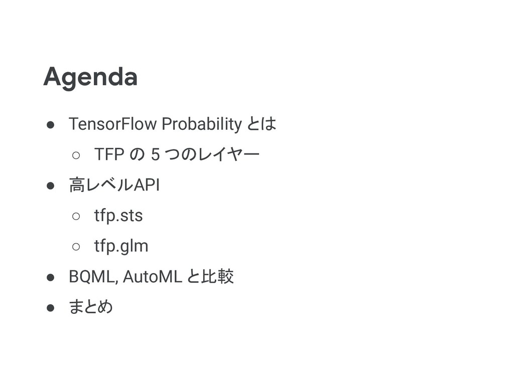
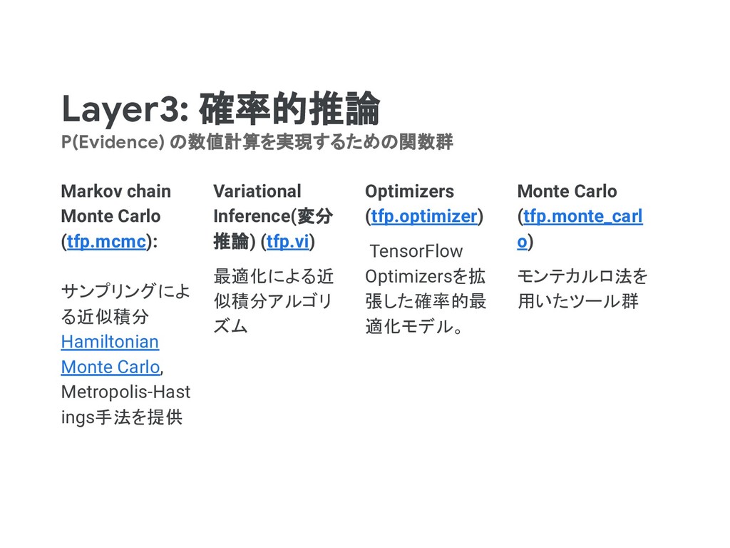
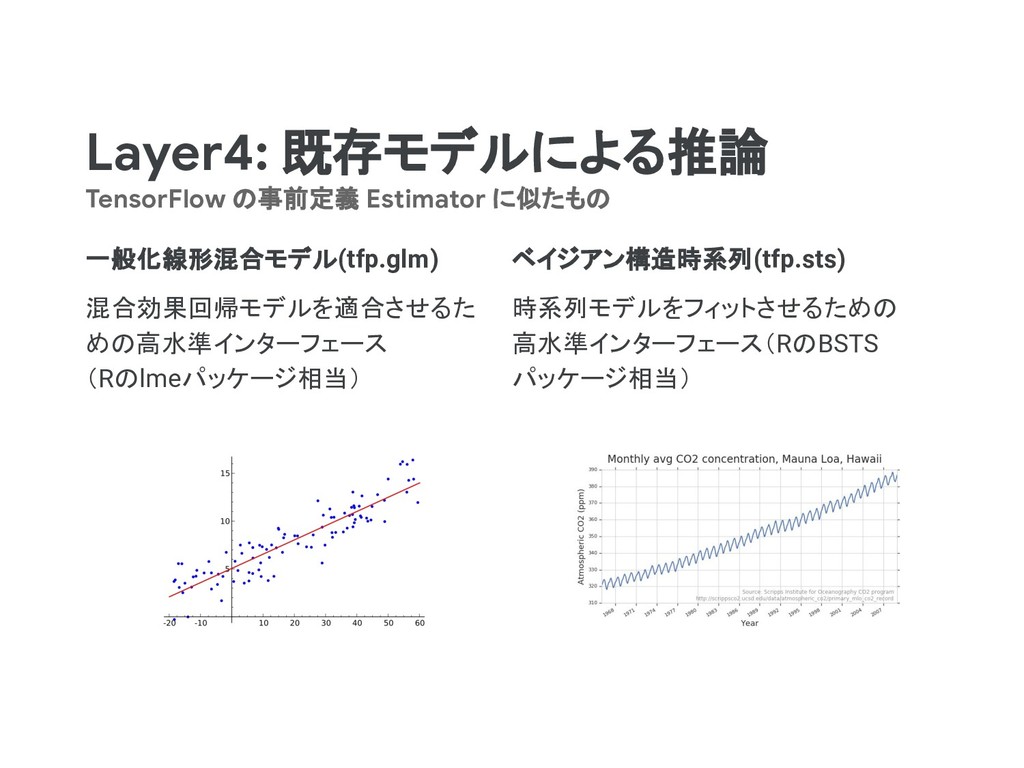
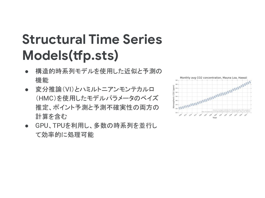
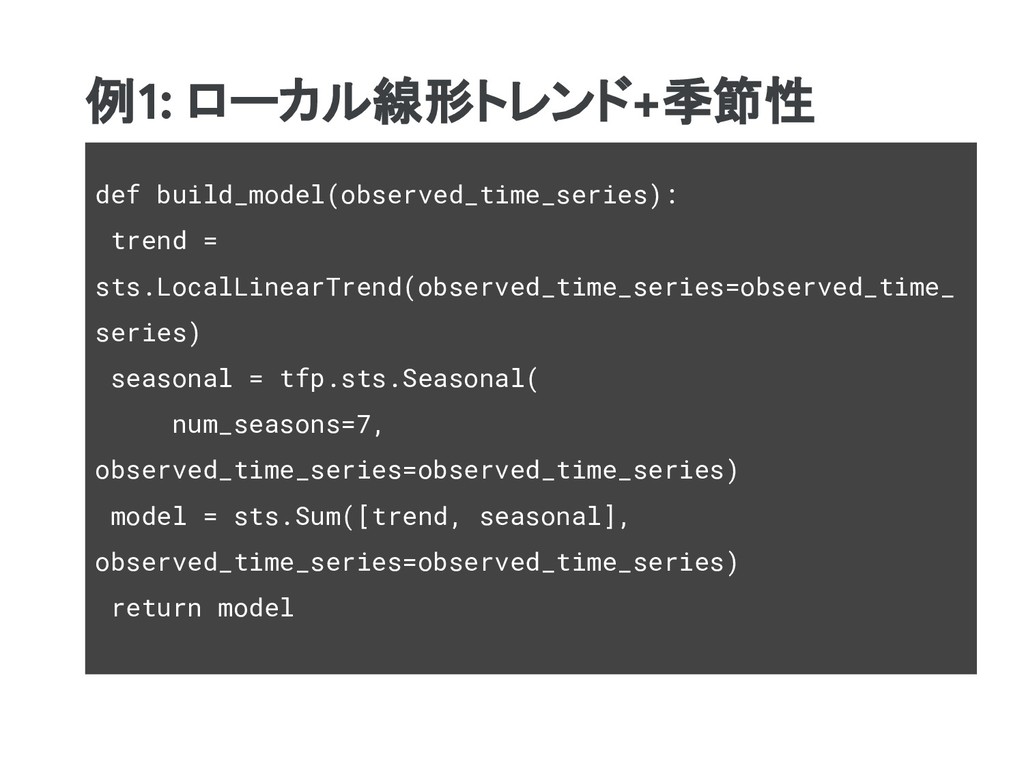
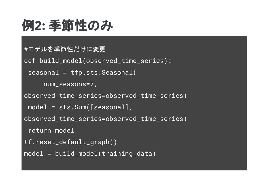
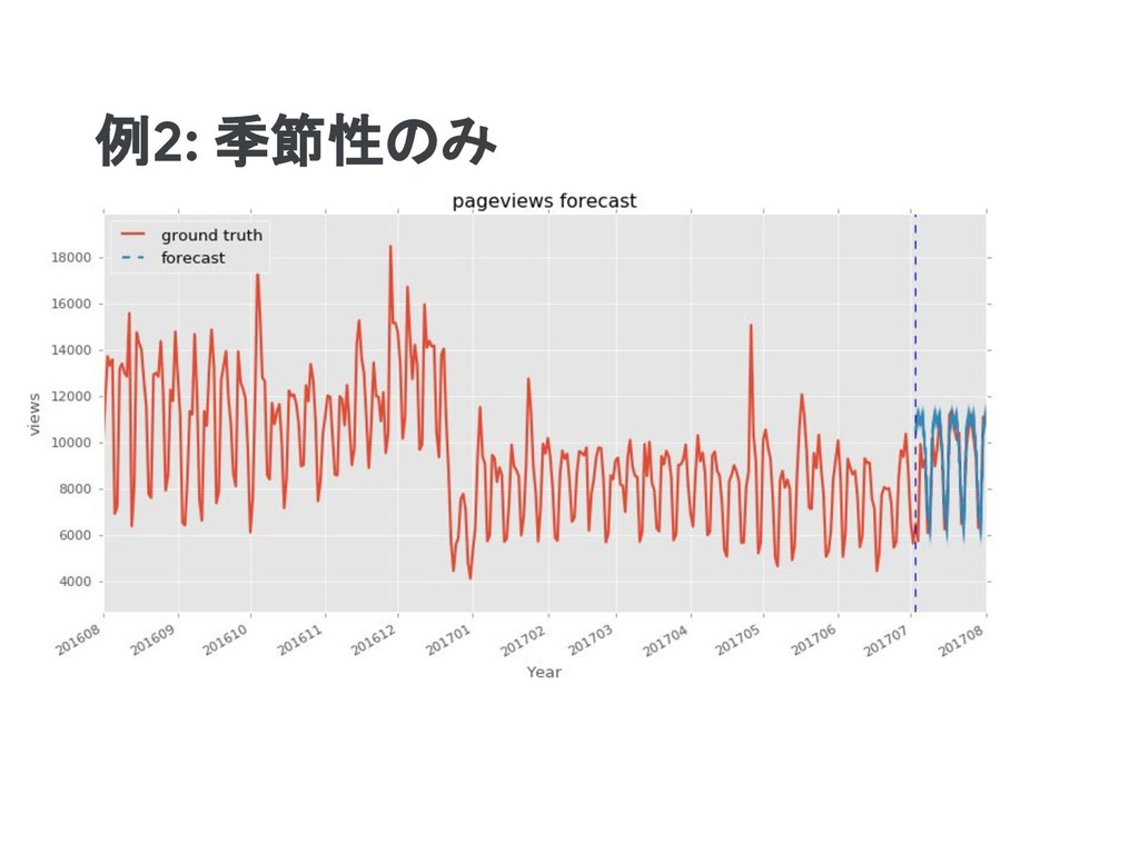
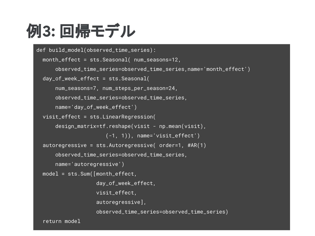
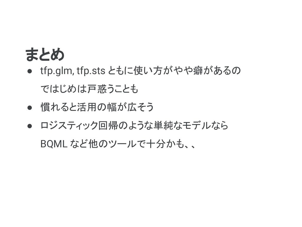
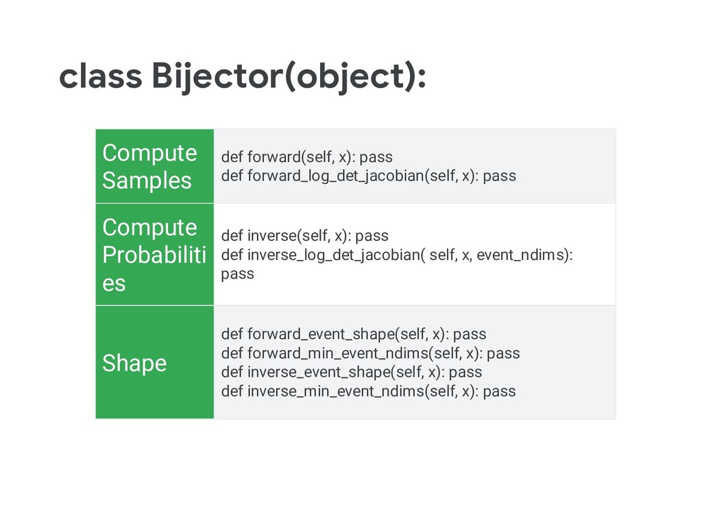
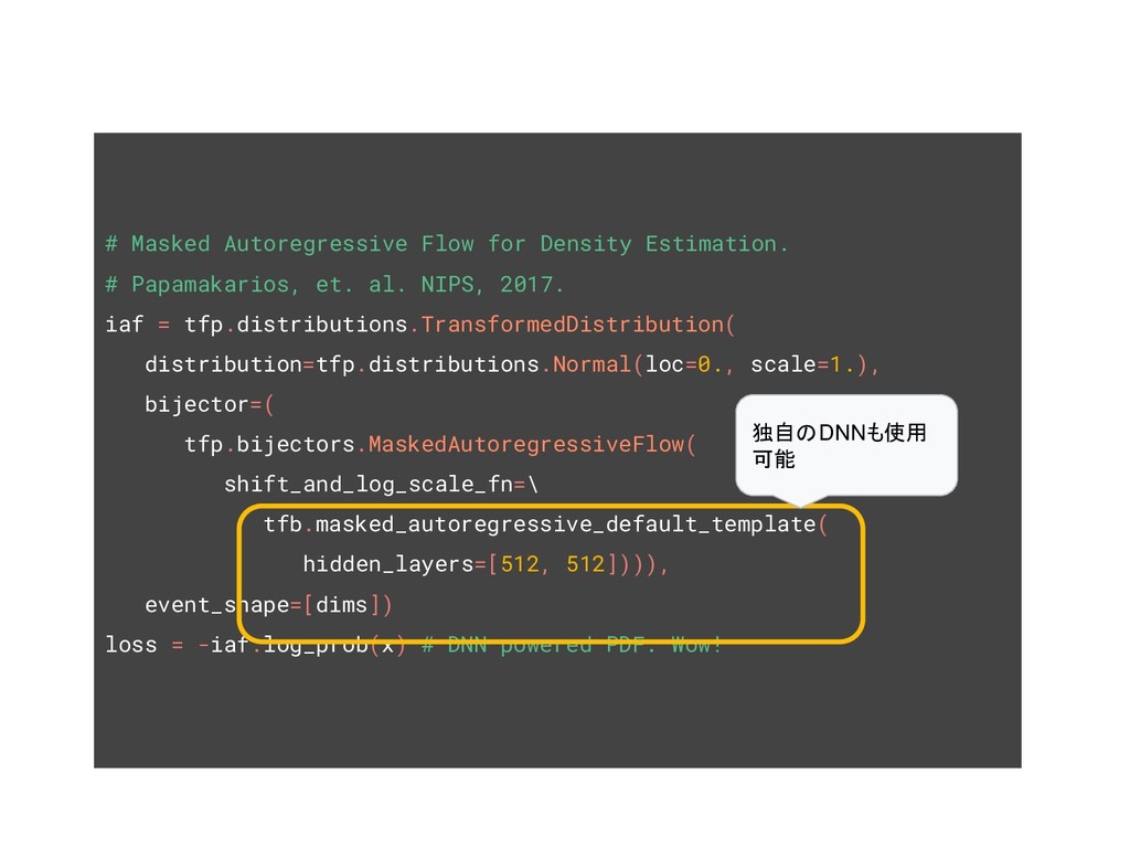
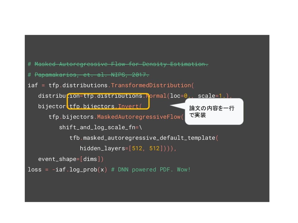
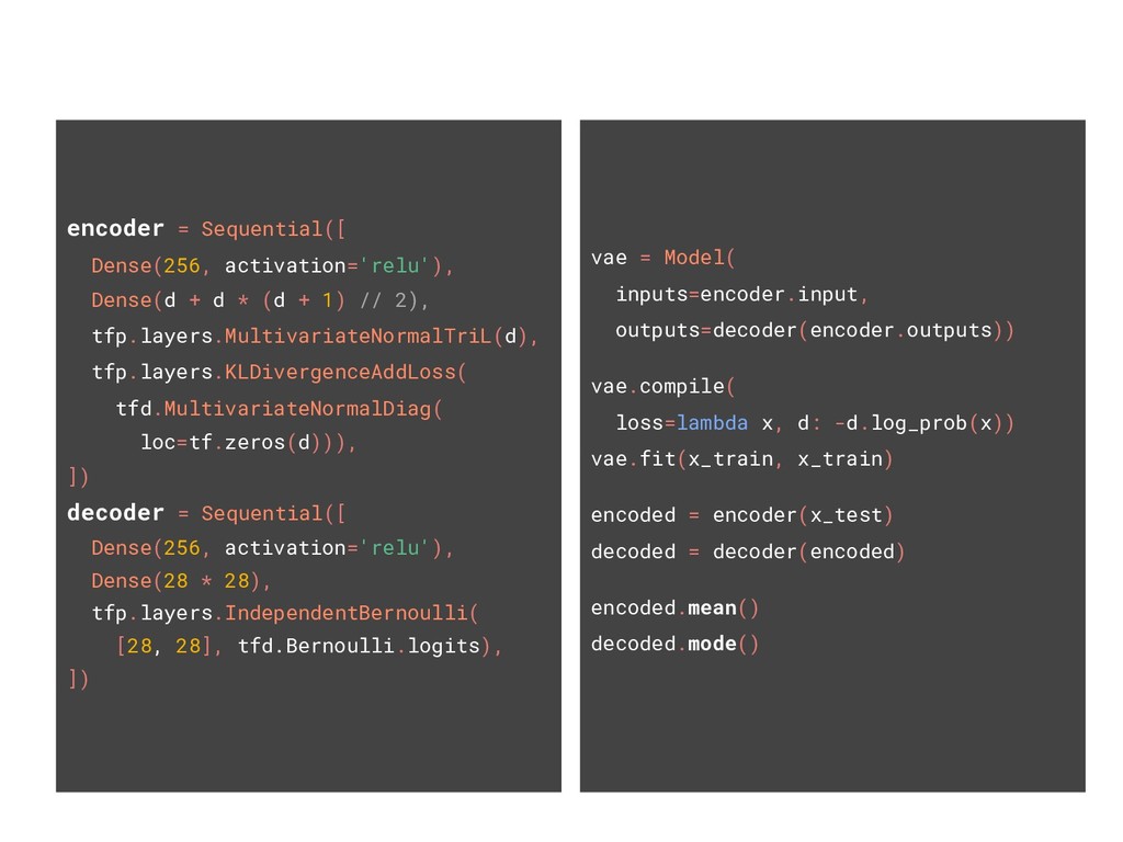
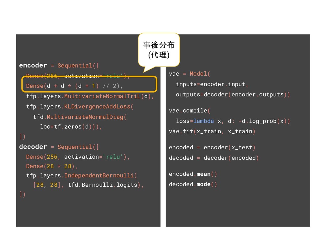
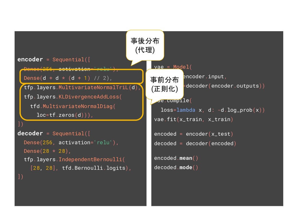
21. 例1: ローカル線形トレンド+季節性 def build_model(observed_time_series): trend = sts.LocalLinearTrend(observed_time_series=observed_time_ series) seasonal = tfp.sts.Seasonal( num_seasons=7, observed_time_series=observed_time_series) model = sts.Sum([trend, seasonal], observed_time_series=observed_time_series) return model
22. 変分推論 # 事後分布を指定 with tf.variable_scope('sts_elbo', reuse=tf.AUTO_REUSE): elbo_loss, variational_posteriors = tfp.sts.build_factored_variational_loss( model, observed_time_series=training_data) # 変分推論で変分損失を最小化 num_variational_steps = 201 # @param { isTemplate: true} num_variational_steps = int(num_variational_steps) train_vi = tf.train.AdamOptimizer(1).minimize(elbo_loss) with tf.Session() as sess: sess.run(tf.global_variables_initializer()) for i in range(num_variational_steps): _, elbo_ = sess.run((train_vi, elbo_loss)) if i % 20 == 0: print("step {} -ELBO {}".format(i, elbo_)) # Draw samples from the variational posterior. q_samples_ga360_ = sess.run({k: q.sample(50) for k, q in variational_posteriors.items()})
23. 例1: ローカル線形トレンド+ 季節性
24. 例2: 季節性 み #モデルを季節性だけに変更 def build_model(observed_time_series): seasonal = tfp.sts.Seasonal( num_seasons=7, observed_time_series=observed_time_series) model = sts.Sum([seasonal], observed_time_series=observed_time_series) return model tf.reset_default_graph() model = build_model(training_data)
25. 例2: 季節性 み
26. 例3: 回帰モデル
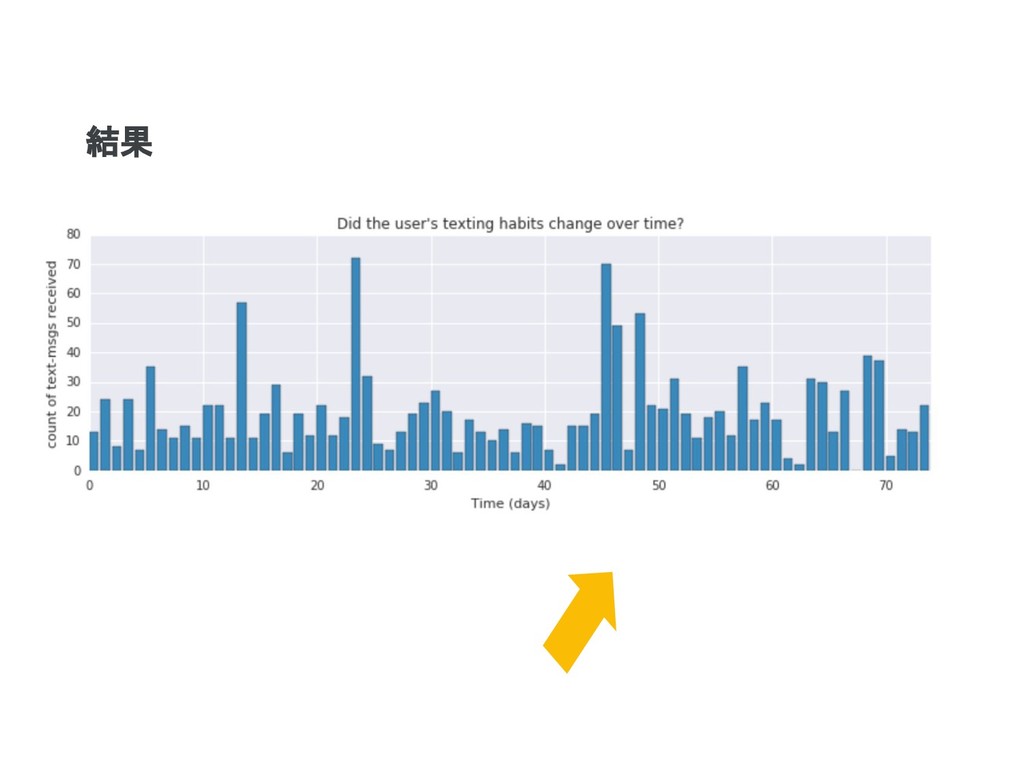
27. 例3: 回帰モデル def build_model(observed_time_series): month_effect = sts.Seasonal( num_seasons=12, observed_time_series=observed_time_series,name='month_effect') day_of_week_effect = sts.Seasonal( num_seasons=7, num_steps_per_season=24, observed_time_series=observed_time_series, name='day_of_week_effect') visit_effect = sts.LinearRegression( design_matrix=tf.reshape(visit - np.mean(visit), (-1, 1)), name='visit_effect') autoregressive = sts.Autoregressive( order=1, #AR(1) observed_time_series=observed_time_series, name='autoregressive') model = sts.Sum([month_effect, day_of_week_effect, visit_effect, autoregressive], observed_time_series=observed_time_series) return model
28. 例3: 回帰モデル
29. tfp.glm (一般化線形モデル) で コンバージョン予測 Google Analytics BigQuery にエクス ポートされたデータで トランザクション(購買) 有無を予測
30. Google Analytics データイメージ Client ID チャネ ル デバイス セッショ ン 平均滞 在時間 ページ ビュー数 イベント 数 CV 3040.9 3496 Paid Search tablet 2 2:05 4.5 12 1 3040.9 3497 Direct desktop 1 1:05 2 2 0 ページビューから購買有無を予測
31. 一般化線形モデル # データセット読み込み features = X_train.values labels = np.array(y_train,dtype='float64') # model の定義 model = tfp.glm.Bernoulli() # model の訓練 coeffs, linear_response, is_converged, num_iter = tfp.glm.fit( model_matrix=features,# データサンプル response=labels, # 観測された効果 model=model)
32. 予測結果 def sigmoid(x): return 1 / (1 + np.exp(-x)) sigmoid(sess.run(linear_response)) array([0.00394942, 0.00394942, 0.00394942, ..., 0.00441452, 0.00441452, 0.00394942]) X = df[["os", "is_mobile", "country", "pageviews"]] y = df["label"] np.unique(y, return_counts = True) (array([0, 1]), array([15835, 165]))
33. over sampling した場合 from imblearn.over_sampling import RandomOverSampler ros = RandomOverSampler(ratio = {0:16000, 1:16000}) X_resample, y_resample = ros.fit_sample(X_train, y_train) X_resample.shape (32000, 2) ： sess.run(linear_response) Tensor("fit_1/while/Exit_2:0", shape=(2,), dtype=float64) array([-3.40057161, -3.40057161, -3.04961137, ..., 1.16191145, 16.95512205, 3.6186331 ])
34. Confusion matrix from sklearn.metrics import confusion_matrix y_pred=sigmoid(sess.run(linear_response)) labels_pred=np.where(y_pred>0.5,1,0) confusion_matrix(y_resample, labels_pred) array([[14689, 1311], [ 1067, 14933]]) #テストデータで検証 b=sess.run(coeffs) y_pred_test = sigmoid(b[0]+b[1]*X_test) labels_pred_test=np.where(y_pred_test>0.5,1,0) confusion_matrix(y_test, labels_pred_test) array([[2932, 240], [ 1, 27]]) Recall=0.96 (買った人28人中27人適合)
35. ここからが本題(?)です
36. 1 2 3 参考: BigQuery ML BigQuery からデータを 移動せずに 機械学習モデル作成 使い慣れた SQL で 開発 度を向上 一般的な ML タスクと ハイパー パラメータ チューニングを自動化
37. BigQueryML 場合 #standardSQL, oversamplingしたデータを取り込み済み CREATE OR REPLACE MODEL `bqml_codelab.sample_model` OPTIONS(model_type='logistic_reg') AS SELECT label AS label, pageview FROM `bqml_codelab.ga360_oversample_train`
38. 結果 (再現率: 0.9323)
39. 構 化データに最先 端 ML モデルを 自動構築 参考：AutoML Tables
40. 最小限 労力と機械学習 専門知識で、 高品質 カスタム機械学習モデルを構築・デプロイ Google Cloud AutoML と
41. 自動的に最適な ML モデルを採用 Linear, logistic Feedforward DNN Wide and Deep NN Gradient Boosted Decision Tree (GBDT) DNN + GBDT Hybrid Adanet ensemble Neural + Tree Architecture Search ...and more!
42. 結果（再現率: 93.6%）
43. • tfp.glm, tfp.sts ともに使い方がやや癖がある で じめ 戸惑うことも • 慣れると活用 幅が広そう • ロジスティック回帰 ような単純なモデルなら BQML など他 ツールで十分かも、、 まとめ
44. 本日ご紹介したコード bit.ly/tfpglm
45. Thank you!
46. TensorFlow Probability 使い方 Distributions Bijectors Layers / Losses Edward2 MCMC Variational Inference Optimize 推論 モデル構築
47. class Distribution(object): Monte Carlo def sample(self, sample_shape=(), seed=None): 平均に よる近似積分でサンプル抽出 Evaluate def prob(self, value): 値 確率 def cdf(self, value): 累積密度関数 def survival_function(self, value): 1 - cdf。数値 精度が 低下するため、CDFより数値的に安定 Summarize 分布 基本的 な要約統計 def mean(self) def variance(self) def stddev(self) def mode(self) def quantile(self, p) Compare def entropy(self): [ある区間にわたる積分] p（x）log p（x） dx。 def cross_entropy(self, other): 2つ 分布を比較 Shape def event_shape(self): 単一 distribution バッチ要素か ら 描画 形状 def batch_shape(self): 単一 distribution クラスに複数 異なるパラメータ化を使用
48. Hello World! import tensorflow_probability as tfp tfd = tfp.distributions d = tfd.Normal(loc=[-1., 1.], scale=1.) # 分布作成 x = d.sample() # ランダムな点を2つ描画(サンプリング) px = d.prob(x) # density/mass 計算
49. Hello World! import tensorflow_probability as tfp tfd = tfp.distributions d = tfd.Normal(loc=[-1., 1.], scale=1.) x = d.sample() # ランダムな点を2つ描画 px = d.prob(x) # Compute density/mass. 異なる2つ 分布を構築
50. distributionで多様な表現が可能 factorial_mog = tfd.Independent( tfd.MixtureSameFamily( # Uniform weight on each component. mixture_distribution = tfd.Categorical( logits = tf.zeros([num_vars, num_components])), components_distribution =\ tfd.MultivariateNormalDiag( loc=mu, scale_diag=[sigma])), reinterpreted_batch_ndims=1) samples = factorial_mog.sample(1000)
51. ガウス過程 posterior_samples = \ tfp.distributions.GaussianProcessRegressionModel( kernel=tfp.positive_semidefinite_kernels.ExponentiatedQuadratic(), index_points=tf.linspace( -3., 3., 200)[..., tf.newaxis], observation_index_points=x, observations=y, jitter=1e-5).sample(50) # ==> 50 posterior samples conditioned on observed data.
52. TensorFlow Probability 使い方 Distributions Bijectors Layers / Losses Edward2 MCMC Variational Inference Optimize 推論 モデル構築
53. class Bijector(object): Compute Samples def forward(self, x): pass def forward_log_det_jacobian(self, x): pass Compute Probabiliti es def inverse(self, x): pass def inverse_log_det_jacobian( self, x, event_ndims): pass Shape def forward_event_shape(self, x): pass def forward_min_event_ndims(self, x): pass def inverse_event_shape(self, x): pass def inverse_min_event_ndims(self, x): pass
54. Bijectors による Distributions変換 # Masked Autoregressive Flow for Density Estimation. # Papamakarios, et. al. NIPS, 2017. iaf = tfp.distributions.TransformedDistribution( distribution=tfp.distributions.Normal(loc=0., scale=1.), bijector=( tfp.bijectors.MaskedAutoregressiveFlow( shift_and_log_scale_fn=\ tfb.masked_autoregressive_default_template( hidden_layers=[512, 512]))), event_shape=[dims]) loss = -iaf.log_prob(x) # DNN powered PDF. Wow! 独自 DNNも使用 可能
55. Bijectors による Distributions変換 # Masked Autoregressive Flow for Density Estimation. # Papamakarios, et. al. NIPS, 2017. iaf = tfp.distributions.TransformedDistribution( distribution=tfp.distributions.Normal(loc=0., scale=1.), bijector=tfp.bijectors.Invert( tfp.bijectors.MaskedAutoregressiveFlow( shift_and_log_scale_fn=\ tfb.masked_autoregressive_default_template( hidden_layers=[512, 512]))), event_shape=[dims]) loss = -iaf.log_prob(x) # DNN powered PDF. Wow! 論文 内容を一行 で実装
56. 例:異常検知 (“Bayesian Methods for Hackers” by Cameron Davidson-Pilon)
57. TFP でコーディング def joint_log_prob(count_data, lambda_1, lambda_2, tau): alpha = 1. / count_data.mean() rv_lambda = tfd.Exponential(rate=alpha) rv_tau = tfd.Uniform() indices = tf.to_int32( tau * count_data.size <= tf.range(count_data.size)) lambda_ = tf.gather( [lambda_1, lambda_2], indices) rv_x= tfd.Poisson(rate=lambda_) return (rv_lambda.log_prob(lambda_1) + rv_lambda.log_prob(lambda_2) + rv_tau.log_prob(tau) + tf.reduce_sum( rv_x.log_prob(count_data)))
58. TFP でコーディング def joint_log_prob(count_data, lambda_1, lambda_2, tau): alpha = 1. / count_data.mean() rv_lambda = tfd.Exponential(rate=alpha) rv_tau = tfd.Uniform() indices = tf.to_int32( tau * count_data.size <= tf.range(count_data.size)) lambda_ = tf.gather( [lambda_1, lambda_2], indices) rv_x= tfd.Poisson(rate=lambda_) return (rv_lambda.log_prob(lambda_1) + rv_lambda.log_prob(lambda_2) + rv_tau.log_prob(tau) + tf.reduce_sum( rv_x.log_prob(count_data))) 対数密度を計算
59. 事後分布
60. TensorFlow Probability 使い方 Distributions Bijectors Layers / Losses Edward2 MCMC Variational Inference Optimize 推論 モデル構築
61. 事後サンプリング [lambda_1, lambda_2, tau], _ = tfp.mcmc.sample_chain( num_results=int(10e3), num_burnin_steps=int(1e3), current_state=initial_chain_state, kernel=tfp.mcmc.TransformedTransitionKernel( inner_kernel=tfp.mcmc.HamiltonianMonteCarlo( target_log_prob_fn=lambda *s: joint_log_prob(count_data, *s), num_leapfrog_steps=2, step_size=tf.Variable(1.), step_size_update_fn=\ tfp.mcmc.make_simple_step_size_update_policy()), bijector=[ tfp.bijectors.Exp(), # Lambda1 tfp.bijectors.Exp(), # Lambda2 tfp.bijectors.Sigmoid()])) # Tau クロージャで事後対 数密度を非正規化
62. 事後サンプリング [lambda_1, lambda_2, tau], _ = tfp.mcmc.sample_chain( num_results=int(10e3), num_burnin_steps=int(1e3), current_state=initial_chain_state, kernel=tfp.mcmc.TransformedTransitionKernel( inner_kernel=tfp.mcmc.HamiltonianMonteCarlo( target_log_prob_fn=lambda *s: joint_log_prob(count_data, *s), num_leapfrog_steps=2, step_size=tf.Variable(1.), step_size_update_fn=\ tfp.mcmc.make_simple_step_size_update_policy()), bijector=[ tfp.bijectors.Exp(), # Lambda1 tfp.bijectors.Exp(), # Lambda2 tfp.bijectors.Sigmoid()])) # Tau セットアップ：変換後 HMCを使用して、後方 から10K サンプルを描 画
63. 事後サンプリング [lambda_1, lambda_2, tau], _ = tfp.mcmc.sample_chain( num_results=int(10e3), num_burnin_steps=int(1e3), current_state=initial_chain_state, kernel=tfp.mcmc.TransformedTransitionKernel( inner_kernel=tfp.mcmc.HamiltonianMonteCarlo( target_log_prob_fn=lambda *s: joint_log_prob(count_data, *s), num_leapfrog_steps=2, step_size=tf.Variable(1.), step_size_update_fn=\ tfp.mcmc.make_simple_step_size_update_policy()), bijector=[ tfp.bijectors.Exp(), # Lambda1 tfp.bijectors.Exp(), # Lambda2 tfp.bijectors.Sigmoid()])) # Tau 確率変数 サポートを 制約 ない実数にマッ ピング HMCサンプルが常に0 を超える確率を持ち、 チェーンを固定
64. 結果
65. Keras による分布 予測 encoder = Sequential([ Dense(256, activation='relu'), Dense(d + d * (d + 1) // 2), tfp.layers.MultivariateNormalTriL(d), tfp.layers.KLDivergenceAddLoss( tfd.MultivariateNormalDiag( loc=tf.zeros(d))), ]) decoder = Sequential([ Dense(256, activation='relu'), Dense(28 * 28), tfp.layers.IndependentBernoulli( [28, 28], tfd.Bernoulli.logits), ]) vae = Model( inputs=encoder.input, outputs=decoder(encoder.outputs)) vae.compile( loss=lambda x, d: -d.log_prob(x)) vae.fit(x_train, x_train) encoded = encoder(x_test) decoded = decoder(encoded) encoded.mean() decoded.mode()
66. Keras による分布 予測 encoder = Sequential([ Dense(256, activation='relu'), Dense(d + d * (d + 1) // 2), tfp.layers.MultivariateNormalTriL(d), tfp.layers.KLDivergenceAddLoss( tfd.MultivariateNormalDiag( loc=tf.zeros(d))), ]) decoder = Sequential([ Dense(256, activation='relu'), Dense(28 * 28), tfp.layers.IndependentBernoulli( [28, 28], tfd.Bernoulli.logits), ]) vae = Model( inputs=encoder.input, outputs=decoder(encoder.outputs)) vae.compile( loss=lambda x, d: -d.log_prob(x)) vae.fit(x_train, x_train) encoded = encoder(x_test) decoded = decoder(encoded) encoded.mean() decoded.mode() 事後分布 (代理)
67. Keras による分布 予測 encoder = Sequential([ Dense(256, activation='relu'), Dense(d + d * (d + 1) // 2), tfp.layers.MultivariateNormalTriL(d), tfp.layers.KLDivergenceAddLoss( tfd.MultivariateNormalDiag( loc=tf.zeros(d))), ]) decoder = Sequential([ Dense(256, activation='relu'), Dense(28 * 28), tfp.layers.IndependentBernoulli( [28, 28], tfd.Bernoulli.logits), ]) vae = Model( inputs=encoder.input, outputs=decoder(encoder.outputs)) vae.compile( loss=lambda x, d: -d.log_prob(x)) vae.fit(x_train, x_train) encoded = encoder(x_test) decoded = decoder(encoded) encoded.mean() decoded.mode() 事後分布 (代理) 事前分布 (正則化)
68. Keras による分布 予測 encoder = Sequential([ Dense(256, activation='relu'), Dense(d + d * (d + 1) // 2), tfp.layers.MultivariateNormalTriL(d), tfp.layers.KLDivergenceAddLoss( tfd.MultivariateNormalDiag( loc=tf.zeros(d))), ]) decoder = Sequential([ Dense(256, activation='relu'), Dense(28 * 28), tfp.layers.IndependentBernoulli( [28, 28], tfd.Bernoulli.logits), ]) vae = Model( inputs=encoder.input, outputs=decoder(encoder.outputs)) vae.compile( loss=lambda x, d: -d.log_prob(x)) vae.fit(x_train, x_train) encoded = encoder(x_test) decoded = decoder(encoded) encoded.mean() decoded.mode() 事後分布 (代理) 事前分布 (正則化) 尤度
69. Keras による分布 予測 encoder = Sequential([ Dense(256, activation='relu'), Dense(d + d * (d + 1) // 2), tfp.layers.MultivariateNormalTriL(d), tfp.layers.KLDivergenceAddLoss( tfd.MultivariateNormalDiag( loc=tf.zeros(d))), ]) decoder = Sequential([ Dense(256, activation='relu'), Dense(28 * 28), tfp.layers.IndependentBernoulli( [28, 28], tfd.Bernoulli.logits), ]) vae = Model( inputs=encoder.input, outputs=decoder(encoder.outputs)) vae.compile( loss=lambda x, d: -d.log_prob(x)) vae.fit(x_train, x_train) encoded = encoder(x_test) decoded = decoder(encoded) encoded.mean() decoded.mode() assemble
70. Keras による分布 予測 encoder = Sequential([ Dense(256, activation='relu'), Dense(d + d * (d + 1) // 2), tfp.layers.MultivariateNormalTriL(d), tfp.layers.KLDivergenceAddLoss( tfd.MultivariateNormalDiag( loc=tf.zeros(d))), ]) decoder = Sequential([ Dense(256, activation='relu'), Dense(28 * 28), tfp.layers.IndependentBernoulli( [28, 28], tfd.Bernoulli.logits), ]) vae = Model( inputs=encoder.input, outputs=decoder(encoder.outputs)) vae.compile( loss=lambda x, d: -d.log_prob(x)) vae.fit(x_train, x_train) encoded = encoder(x_test) decoded = decoder(encoded) encoded.mean() decoded.mode() assemble 学習
71. Keras による分布 予測 encoder = Sequential([ Dense(256, activation='relu'), Dense(d + d * (d + 1) // 2), tfp.layers.MultivariateNormalTriL(d), tfp.layers.KLDivergenceAddLoss( tfd.MultivariateNormalDiag( loc=tf.zeros(d))), ]) decoder = Sequential([ Dense(256, activation='relu'), Dense(28 * 28), tfp.layers.IndependentBernoulli( [28, 28], tfd.Bernoulli.logits), ]) vae = Model( inputs=encoder.input, outputs=decoder(encoder.outputs)) vae.compile( loss=lambda x, d: -d.log_prob(x)) vae.fit(x_train, x_train) encoded = encoder(x_test) decoded = decoder(encoded) encoded.mean() decoded.mode() assemble 学習
72. Keras による分布 予測 encoder = Sequential([ Dense(256, activation='relu'), Dense(d + d * (d + 1) // 2), tfp.layers.MultivariateNormalTriL(d), tfp.layers.KLDivergenceAddLoss( tfd.MultivariateNormalDiag( loc=tf.zeros(d))), ]) decoder = Sequential([ Dense(256, activation='relu'), Dense(28 * 28), tfp.layers.　IndependentBernoulli( [28, 28], tfd.Bernoulli.logits), ]) vae = Model( inputs=encoder.input, outputs=decoder(encoder.outputs)) vae.compile( loss=lambda x, d: -d.log_prob(x)) vae.fit(x_train, x_train) encoded = encoder(x_test) decoded = decoder(encoded) encoded.mean() decoded.mode() assemble 学習 結果