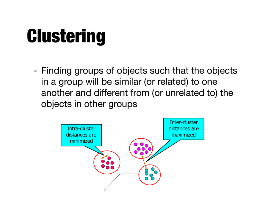
in a group will be similar (or related) to one another and different from (or unrelated to) the objects in other groups Inter-cluster distances are maximized Intra-cluster distances are minimized
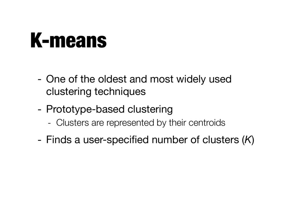
- Business (segmenting customers for additional analysis and marketing activities) - Web (clustering search results into subcategories) - For utility - Some clustering techniques characterize each cluster in terms of a cluster prototype - These prototypes can be used as a basis for a number of data analysis and processing techniques
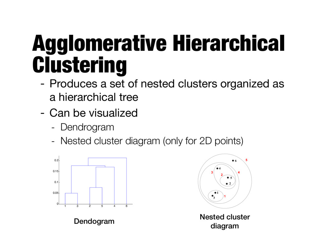
clusters such that each data object is in exactly one cluster - Hierarchical: a set of nested clusters organized as a hierarchical tree - Exclusive vs. non-exclusive - Whether points may belong to a single or multiple clusters
some cases, we only want to cluster some of the data - Fuzzy vs. non-fuzzy - In fuzzy clustering, a point belongs to every cluster with some weight between 0 and 1 - Weights must sum to 1 - Probabilistic clustering has similar characteristics
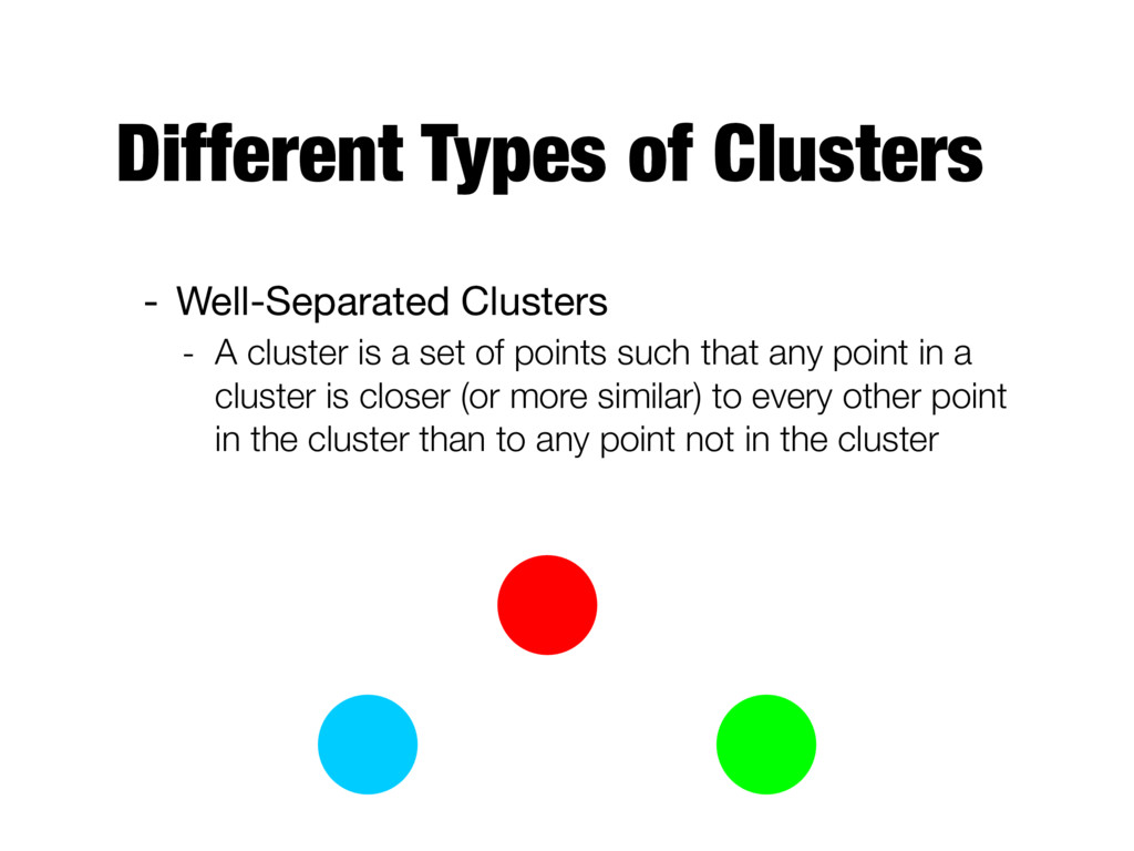
is a set of points such that any point in a cluster is closer (or more similar) to every other point in the cluster than to any point not in the cluster
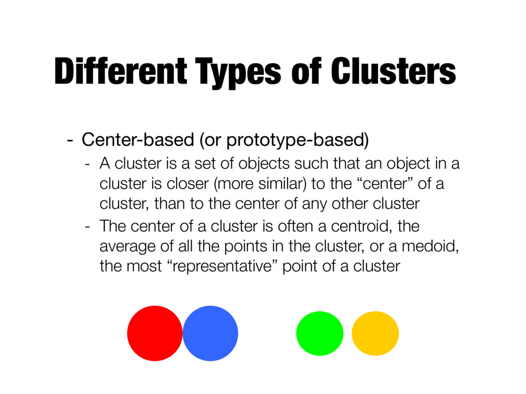
cluster is a set of objects such that an object in a cluster is closer (more similar) to the “center” of a cluster, than to the center of any other cluster - The center of a cluster is often a centroid, the average of all the points in the cluster, or a medoid, the most “representative” point of a cluster
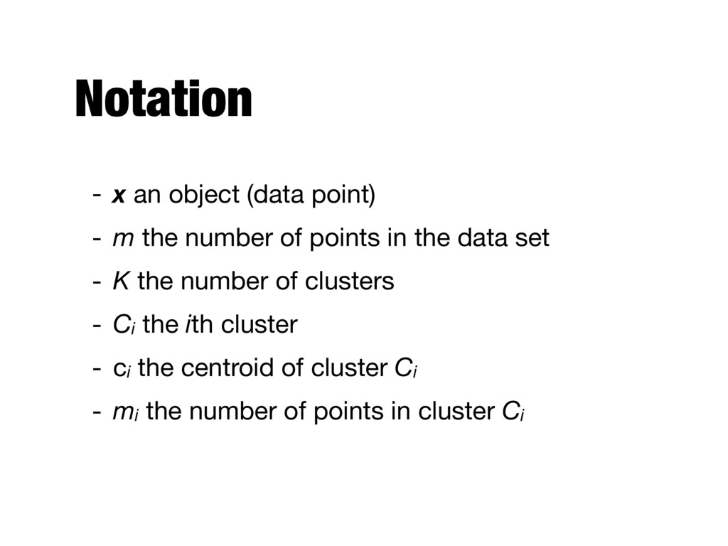
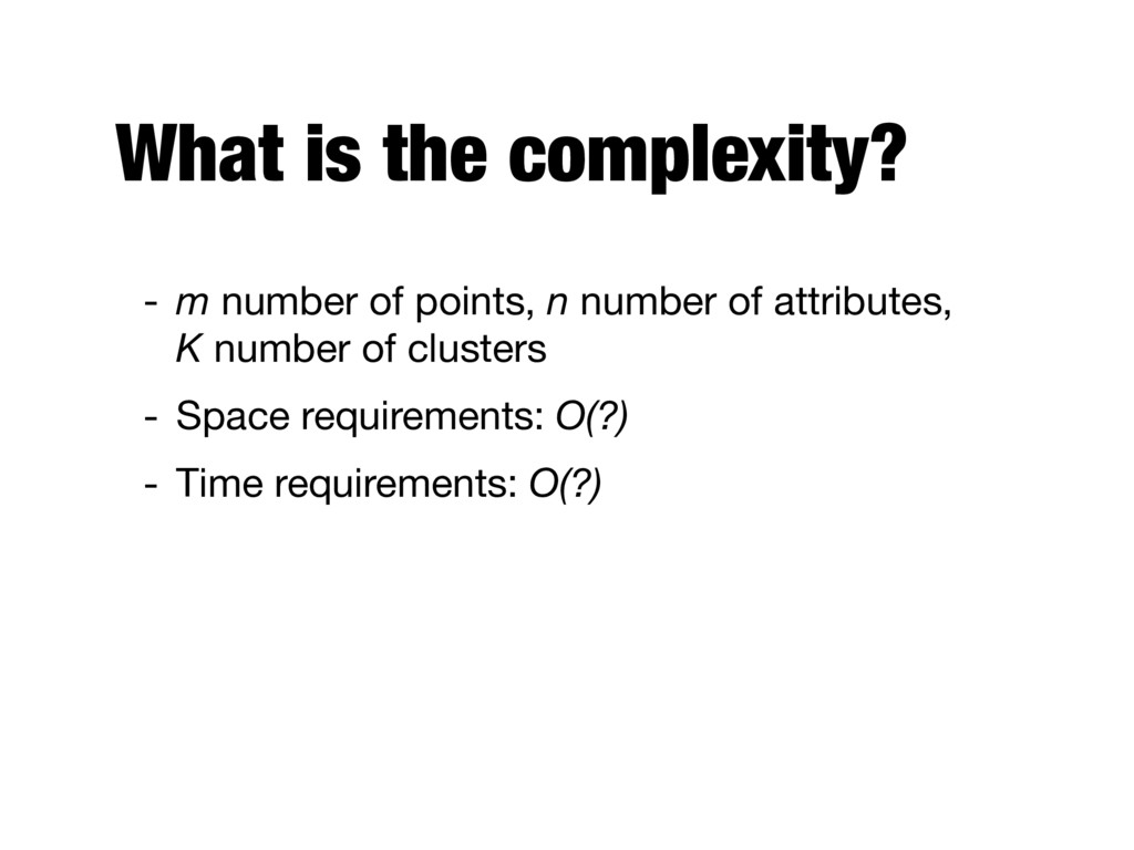
number of points in the data set - K the number of clusters - Ci the ith cluster - ci the centroid of cluster Ci - mi the number of points in cluster Ci
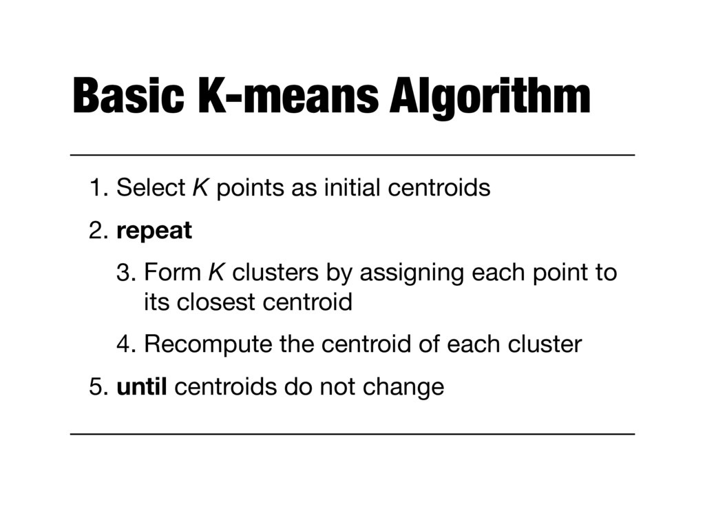
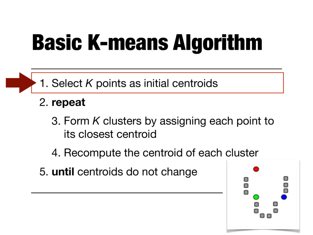
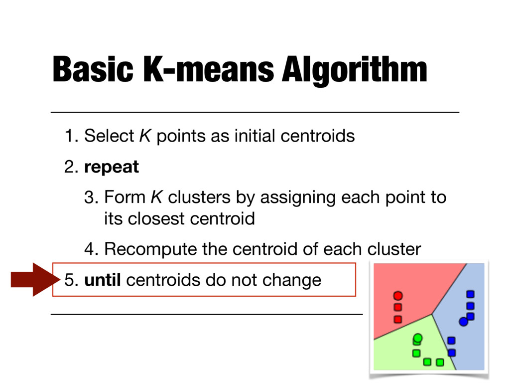
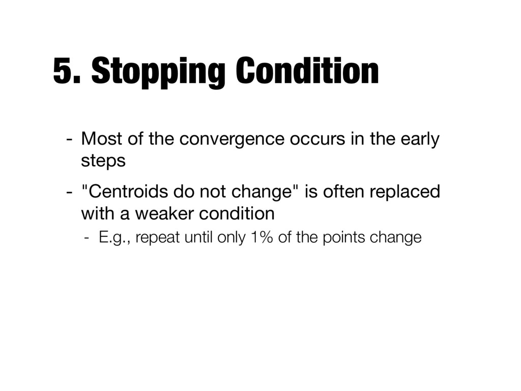
2. repeat 3. Form K clusters by assigning each point to its closest centroid 4. Recompute the centroid of each cluster 5. until centroids do not change
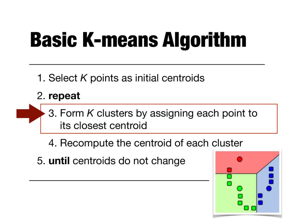
2. repeat 3. Form K clusters by assigning each point to its closest centroid 4. Recompute the centroid of each cluster 5. until centroids do not change
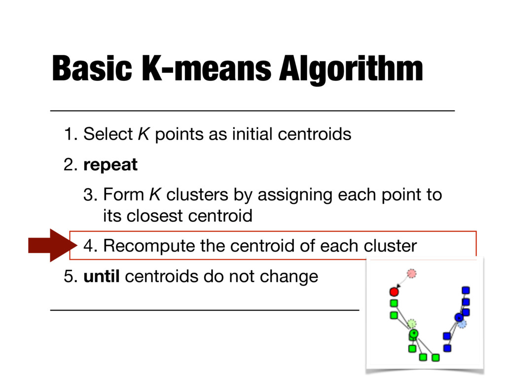
2. repeat 3. Form K clusters by assigning each point to its closest centroid 4. Recompute the centroid of each cluster 5. until centroids do not change
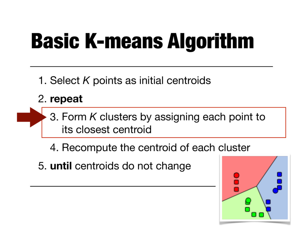
2. repeat 3. Form K clusters by assigning each point to its closest centroid 4. Recompute the centroid of each cluster 5. until centroids do not change
2. repeat 3. Form K clusters by assigning each point to its closest centroid 4. Recompute the centroid of each cluster 5. until centroids do not change
2. repeat 3. Form K clusters by assigning each point to its closest centroid 4. Recompute the centroid of each cluster 5. until centroids do not change
a proximity measure that quantifies the notion of "closest" - Usually chosen to be simple - Has to be calculated repeatedly - See distance functions from Lecture 1 - E.g., Euclidean distance
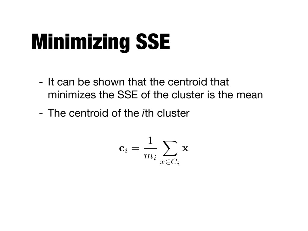
what is it that we want minimize/maximize - Once the objective function and the proximity measure are defined, we can define mathematically the centroid we should choose - E.g., minimize the squared distance of each point to its closest centroid
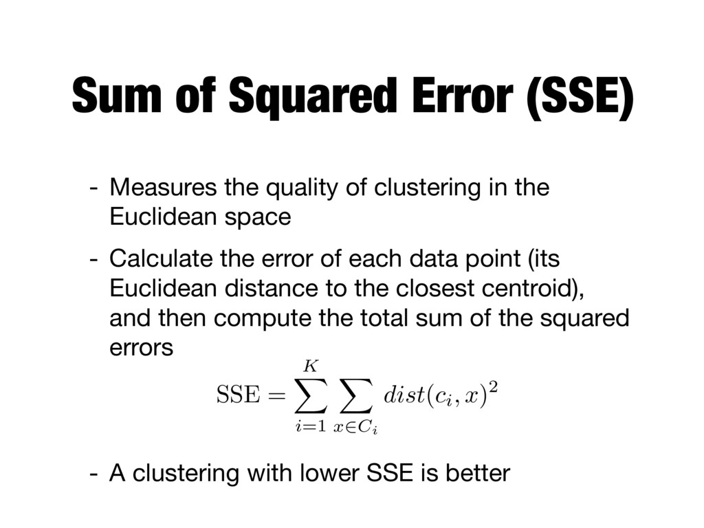
clustering in the Euclidean space - Calculate the error of each data point (its Euclidean distance to the closest centroid), and then compute the total sum of the squared errors - A clustering with lower SSE is better SSE = K X i =1 X x 2 Ci dist ( ci, x )2
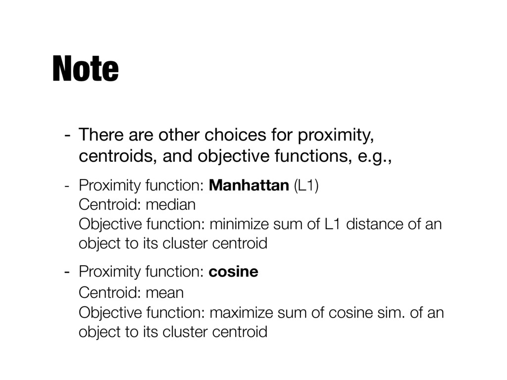
objective functions, e.g., - Proximity function: Manhattan (L1) Centroid: median Objective function: minimize sum of L1 distance of an object to its cluster centroid - Proximity function: cosine Centroid: mean Objective function: maximize sum of cosine sim. of an object to its cluster centroid
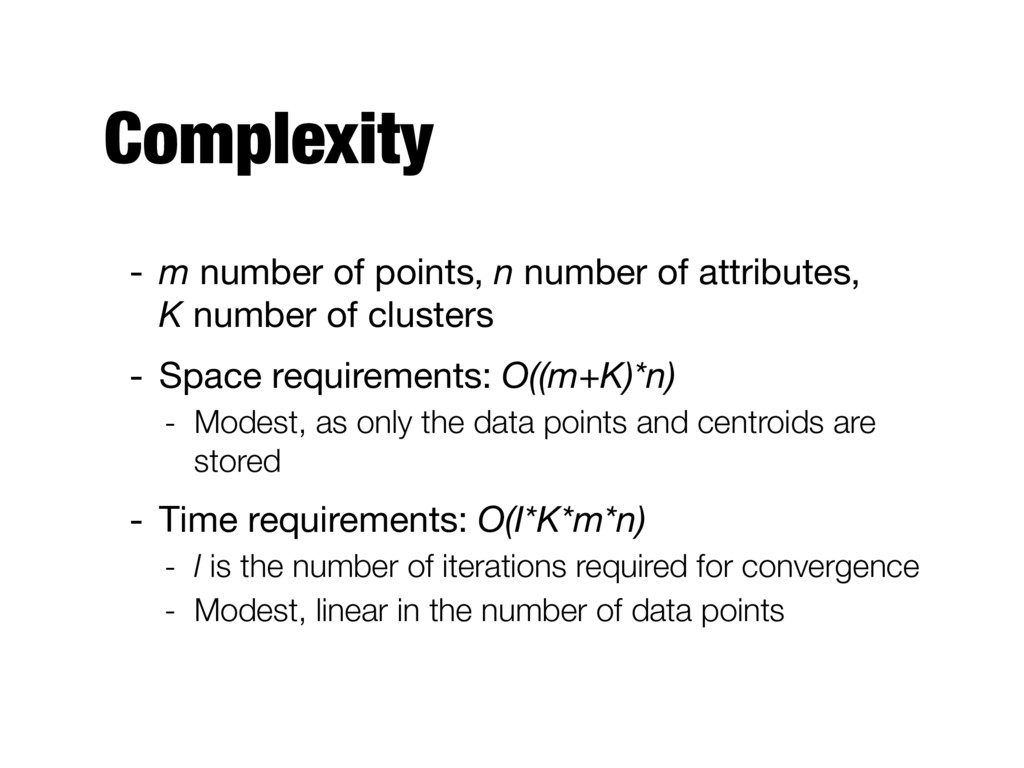
K number of clusters - Space requirements: O((m+K)*n) - Modest, as only the data points and centroids are stored - Time requirements: O(I*K*m*n) - I is the number of iterations required for convergence - Modest, linear in the number of data points
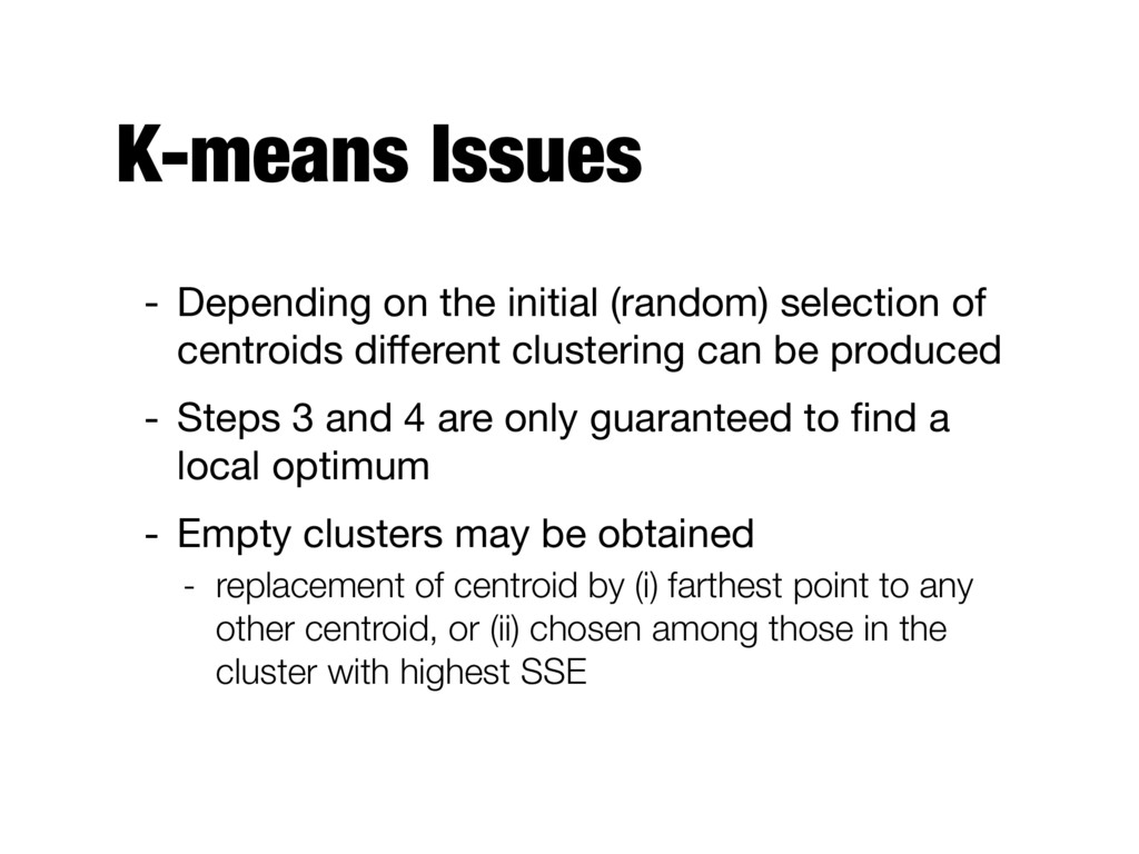
centroids different clustering can be produced - Steps 3 and 4 are only guaranteed to find a local optimum - Empty clusters may be obtained - replacement of centroid by (i) farthest point to any other centroid, or (ii) chosen among those in the cluster with highest SSE
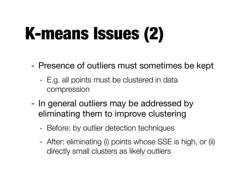
kept - E.g. all points must be clustered in data compression - In general outliers may be addressed by eliminating them to improve clustering - Before: by outlier detection techniques - After: eliminating (i) points whose SSE is high, or (ii) directly small clusters as likely outliers
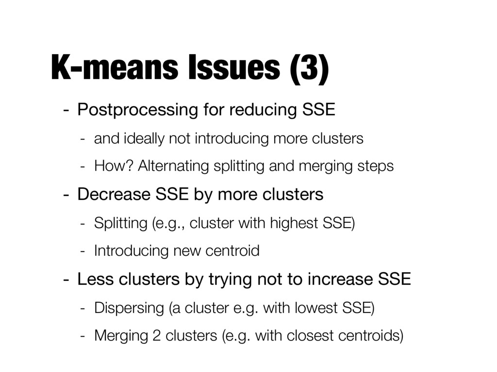
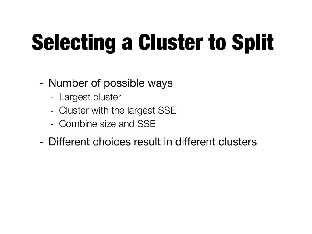
ideally not introducing more clusters - How? Alternating splitting and merging steps - Decrease SSE by more clusters - Splitting (e.g., cluster with highest SSE) - Introducing new centroid - Less clusters by trying not to increase SSE - Dispersing (a cluster e.g. with lowest SSE) - Merging 2 clusters (e.g. with closest centroids)
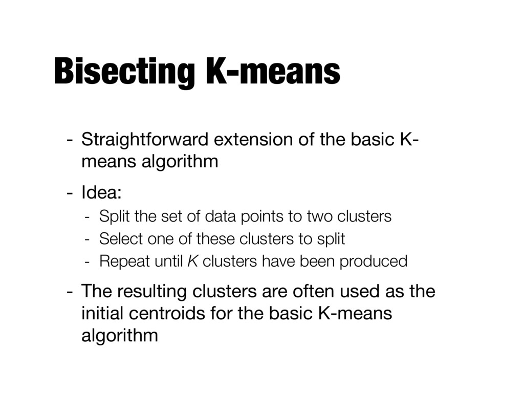
algorithm - Idea: - Split the set of data points to two clusters - Select one of these clusters to split - Repeat until K clusters have been produced - The resulting clusters are often used as the initial centroids for the basic K-means algorithm
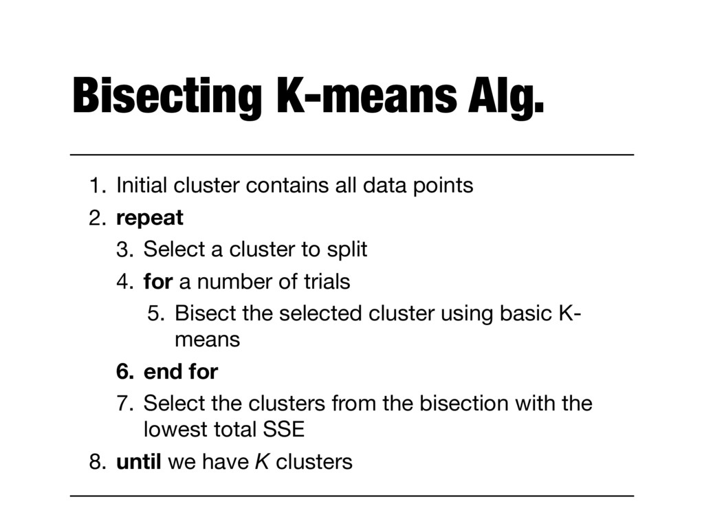
2. repeat 3. Select a cluster to split 4. for a number of trials 5. Bisect the selected cluster using basic K- means 6. end for 7. Select the clusters from the bisection with the lowest total SSE 8. until we have K clusters
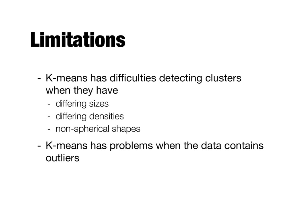
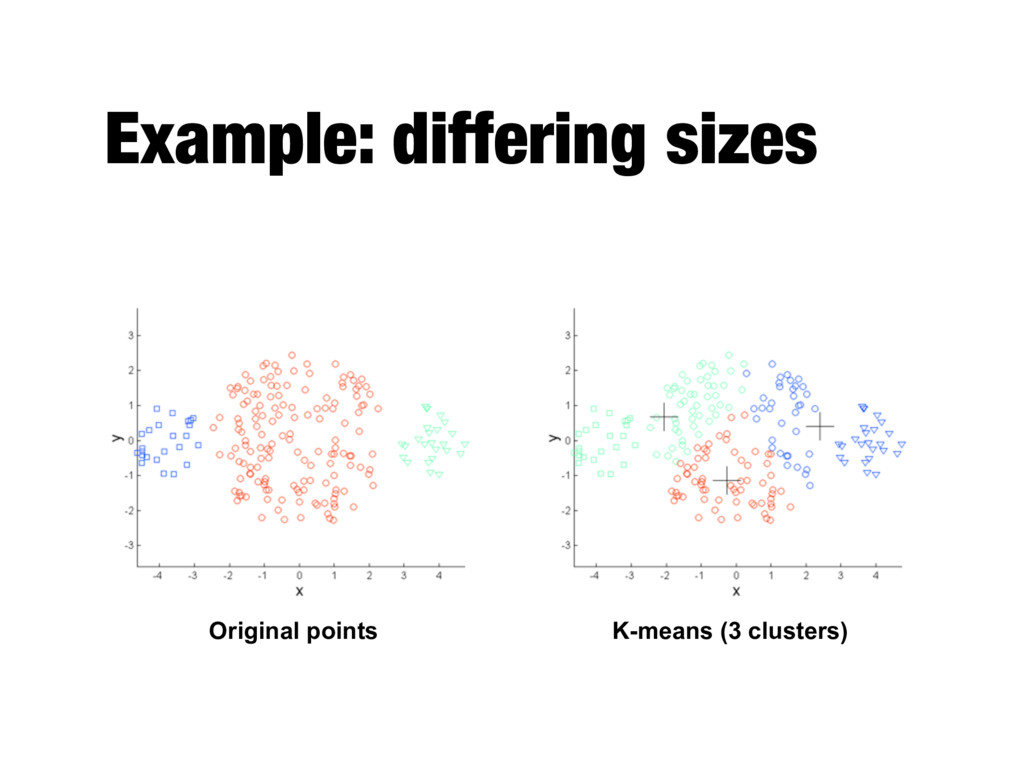
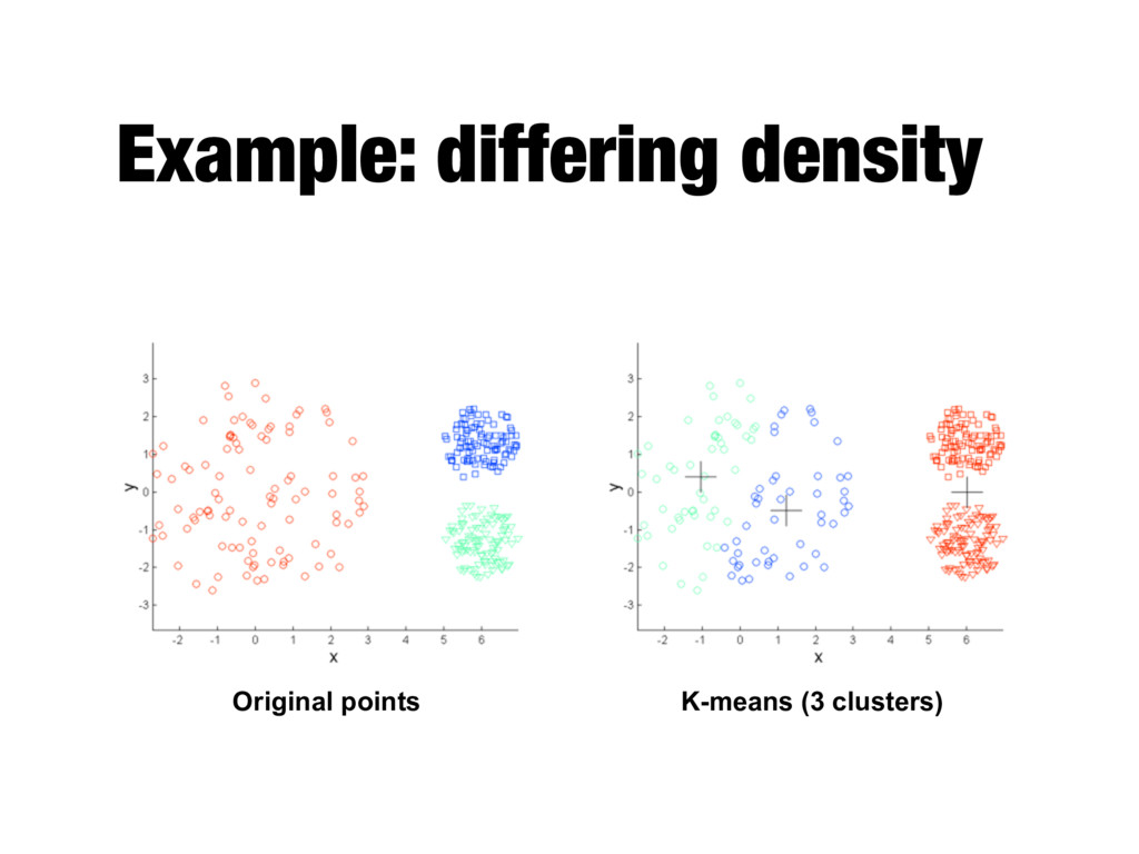
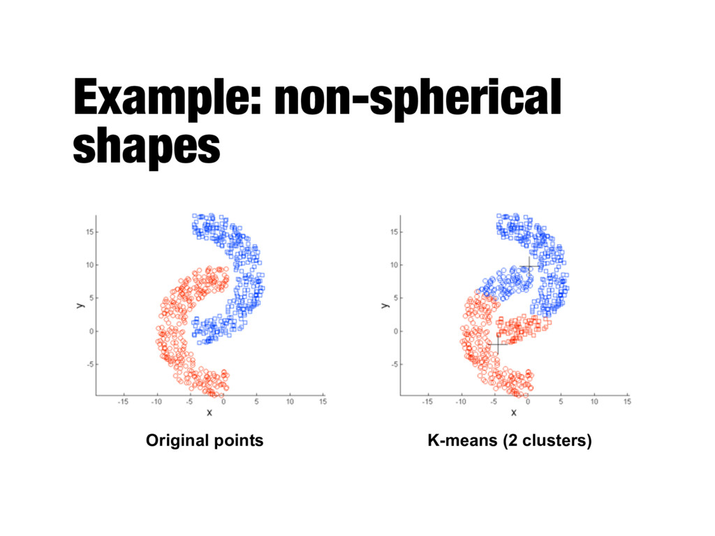
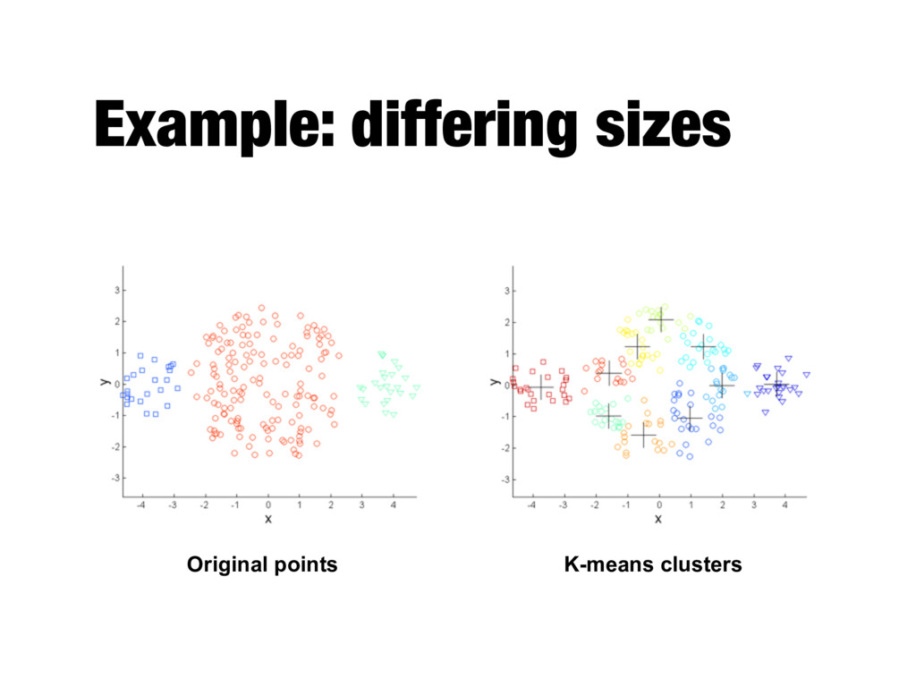
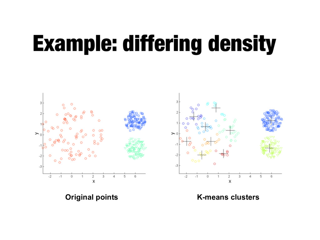
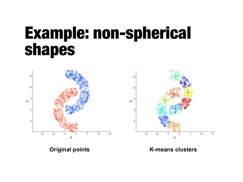
relatively small (K<<m) - Bisecting variant is even more efficient and less susceptible to initialization problems - Cannot handle certain types of clusters - Problems can be overcome by generating more (sub)clusters - Has trouble with data that contains outliers - Outlier detection and removal can help
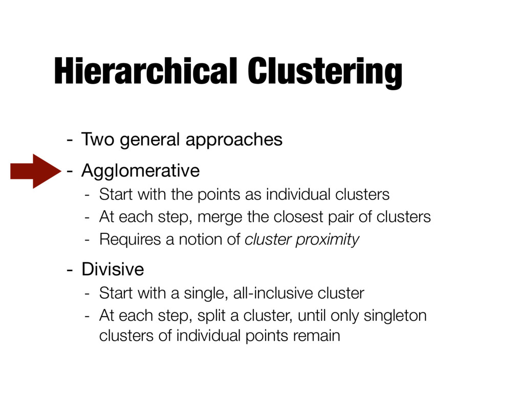
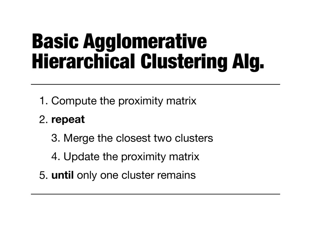
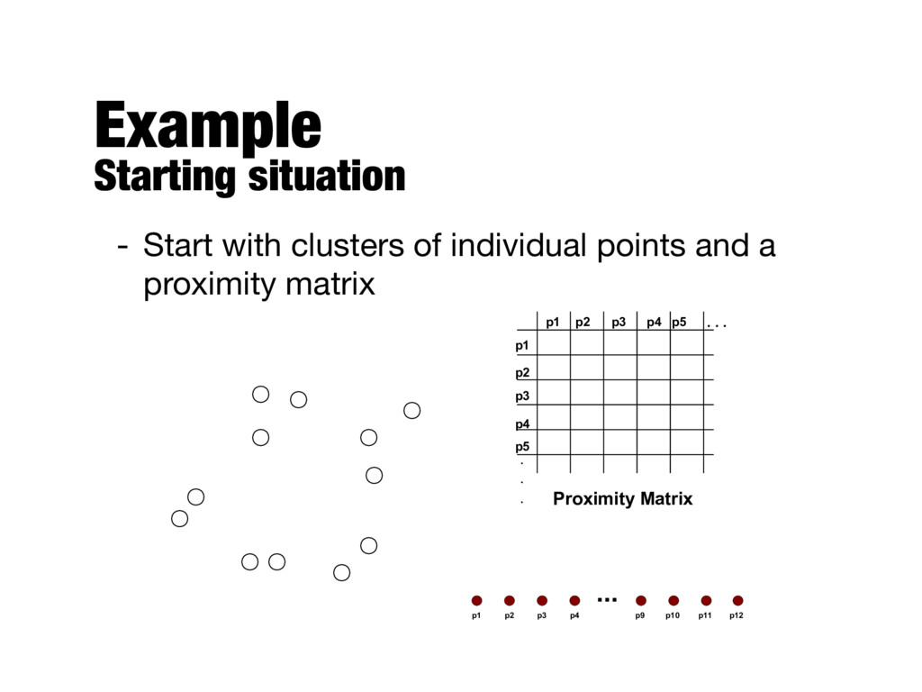
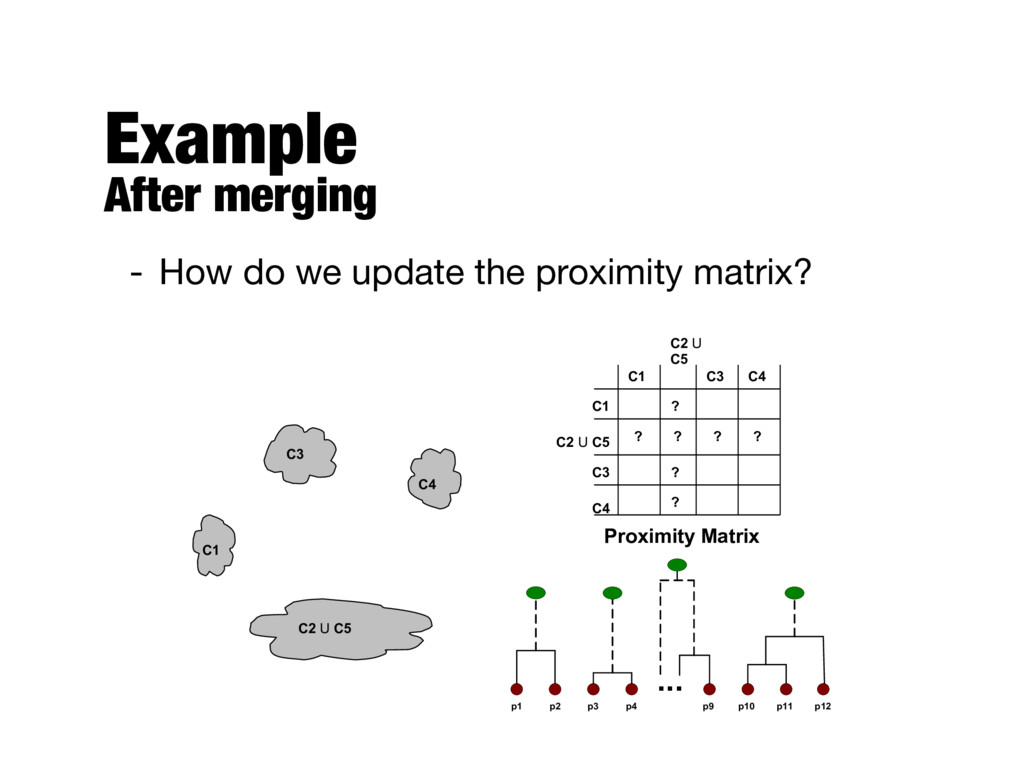
with the points as individual clusters - At each step, merge the closest pair of clusters - Requires a notion of cluster proximity - Divisive - Start with a single, all-inclusive cluster - At each step, split a cluster, until only singleton clusters of individual points remain
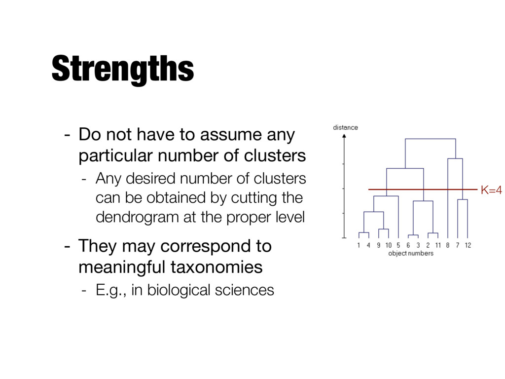
of clusters - Any desired number of clusters can be obtained by cutting the dendrogram at the proper level - They may correspond to meaningful taxonomies - E.g., in biological sciences K=4
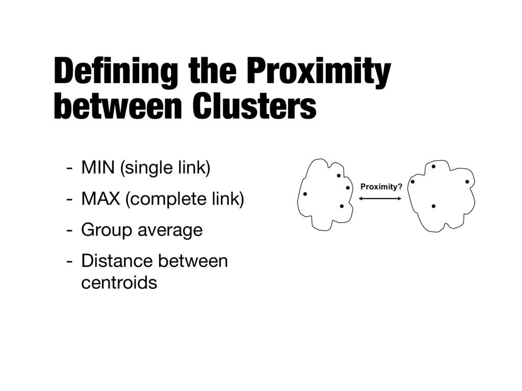
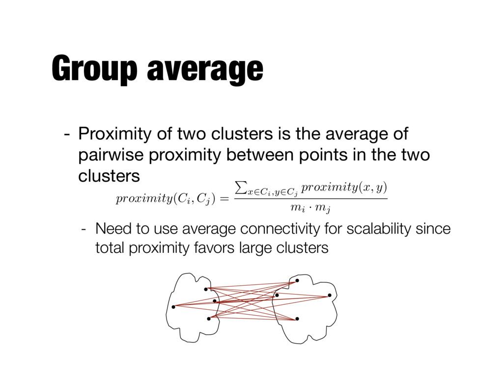
of pairwise proximity between points in the two clusters - Need to use average connectivity for scalability since total proximity favors large clusters proximity ( Ci, Cj ) = P x 2 Ci,y 2 Cj proximity ( x, y ) mi · mj
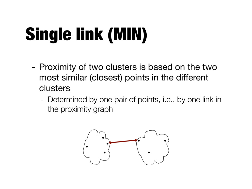
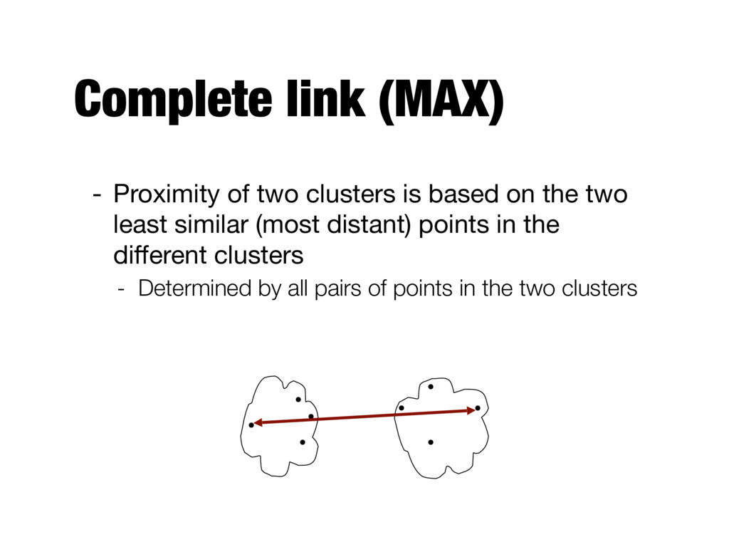
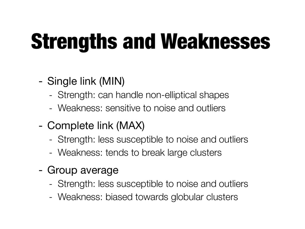
handle non-elliptical shapes - Weakness: sensitive to noise and outliers - Complete link (MAX) - Strength: less susceptible to noise and outliers - Weakness: tends to break large clusters - Group average - Strength: less susceptible to noise and outliers - Weakness: biased towards globular clusters
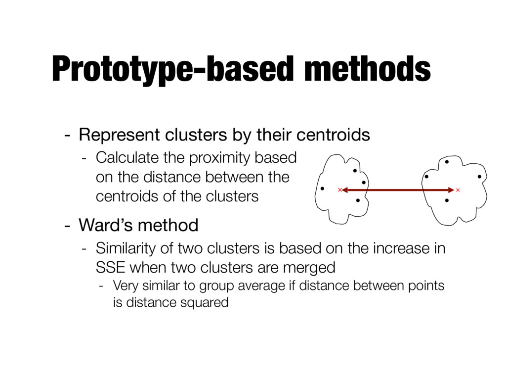
the proximity based on the distance between the centroids of the clusters - Ward’s method - Similarity of two clusters is based on the increase in SSE when two clusters are merged - Very similar to group average if distance between points is distance squared × ×
optimized - No problems with choosing initial points or running into local minima - Merging decisions are final - Once a decision is made to combine two clusters, it cannot be undone
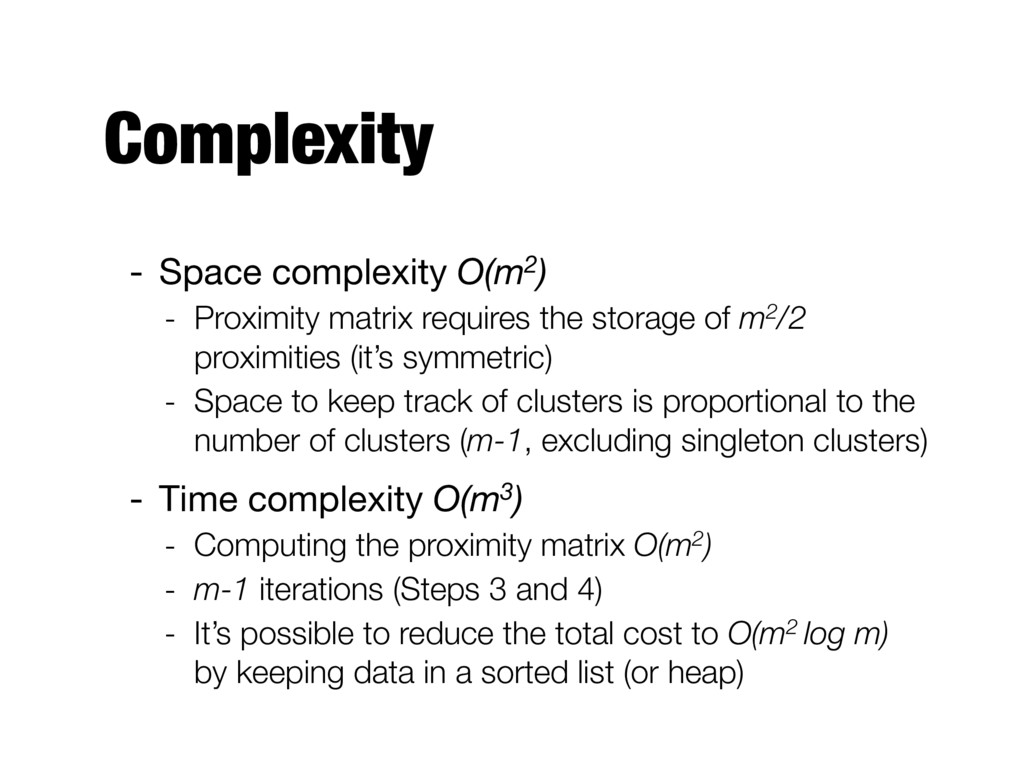
storage of m2/2 proximities (it’s symmetric) - Space to keep track of clusters is proportional to the number of clusters (m-1, excluding singleton clusters) - Time complexity O(m3) - Computing the proximity matrix O(m2) - m-1 iterations (Steps 3 and 4) - It’s possible to reduce the total cost to O(m2 log m) by keeping data in a sorted list (or heap)