DAT630/2017 [DM] Introduction & Data

University of Stavanger, DAT630, 2017 Autumn
lecture by Darío Garigliotti

Transcript

1. DAT630
 Introduction & Data Darío Garigliotti | University of Stavanger 11/09/2017 Introduction to Data Mining, Chapters 1-2
2. Introduction
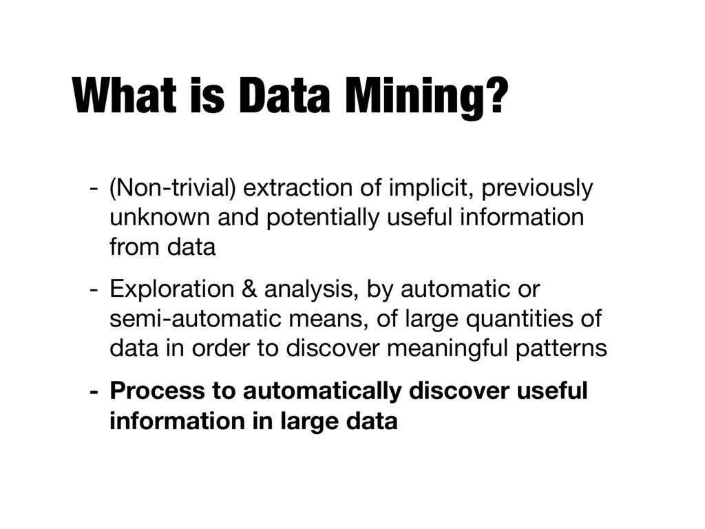
3. What is Data Mining? - (Non-trivial) extraction of implicit, previously unknown and potentially useful information from data - Exploration & analysis, by automatic or 
 semi-automatic means, of large quantities of data in order to discover meaningful patterns - Process to automatically discover useful information in large data
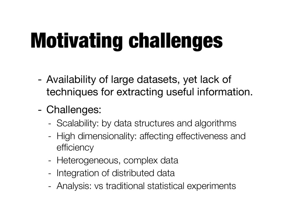
4. Motivating challenges - Availability of large datasets, yet lack of techniques for extracting useful information. - Challenges: - Scalability: by data structures and algorithms - High dimensionality: affecting effectiveness and efficiency - Heterogeneous, complex data - Integration of distributed data - Analysis: vs traditional statistical experiments
5. Typical Workflow
6. Data Mining Tasks - Predictive methods - Use some variables to predict unknown or future values of other variables - Descriptive methods - Find human-interpretable patterns that describe the data
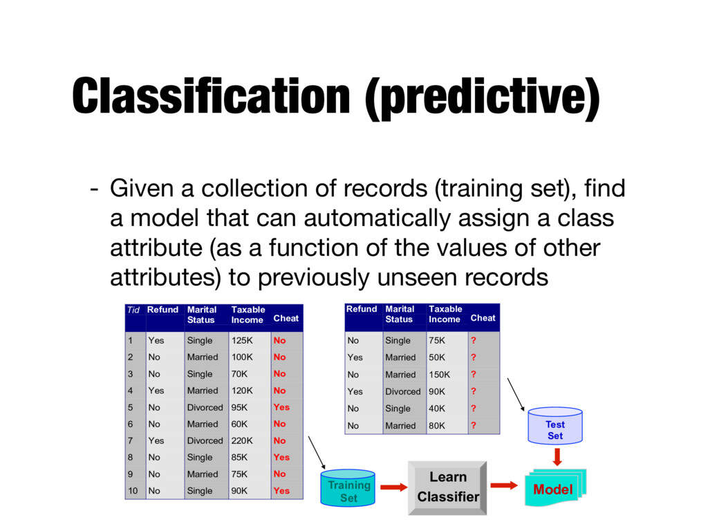
7. Classification (predictive) - Given a collection of records (training set), find a model that can automatically assign a class attribute (as a function of the values of other attributes) to previously unseen records Tid Refund Marital Status Taxable Income Cheat 1 Yes Single 125K No 2 No Married 100K No 3 No Single 70K No 4 Yes Married 120K No 5 No Divorced 95K Yes 6 No Married 60K No 7 Yes Divorced 220K No 8 No Single 85K Yes 9 No Married 75K No 10 No Single 90K Yes 10 Refund Marital Status Taxable Income Cheat No Single 75K ? Yes Married 50K ? No Married 150K ? Yes Divorced 90K ? No Single 40K ? No Married 80K ? 10 Test Set Training Set Model Learn Classifier
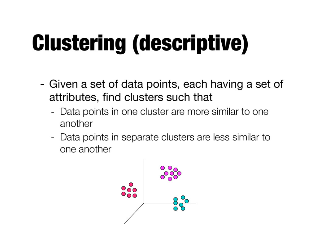
8. Clustering (descriptive) - Given a set of data points, each having a set of attributes, find clusters such that - Data points in one cluster are more similar to one another - Data points in separate clusters are less similar to one another
9. Types of Data
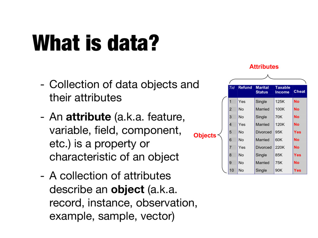
10. What is data? - Collection of data objects and their attributes - An attribute (a.k.a. feature, variable, field, component, etc.) is a property or characteristic of an object - A collection of attributes describe an object (a.k.a. record, instance, observation, example, sample, vector) Tid Refund Marital Status Taxable Income Cheat 1 Yes Single 125K No 2 No Married 100K No 3 No Single 70K No 4 Yes Married 120K No 5 No Divorced 95K Yes 6 No Married 60K No 7 Yes Divorced 220K No 8 No Single 85K Yes 9 No Married 75K No 10 No Single 90K Yes 10 Attributes Objects
11. Attribute properties - The type of an attribute depends on which of the following properties it possesses: - Distinctness: = != - Order: < > <= >= - Addition: + - - Multiplication: * /
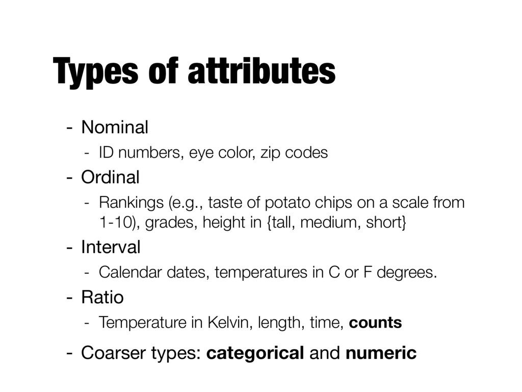
12. Types of attributes - Nominal - ID numbers, eye color, zip codes - Ordinal - Rankings (e.g., taste of potato chips on a scale from 1-10), grades, height in {tall, medium, short} - Interval - Calendar dates, temperatures in C or F degrees. - Ratio - Temperature in Kelvin, length, time, counts - Coarser types: categorical and numeric
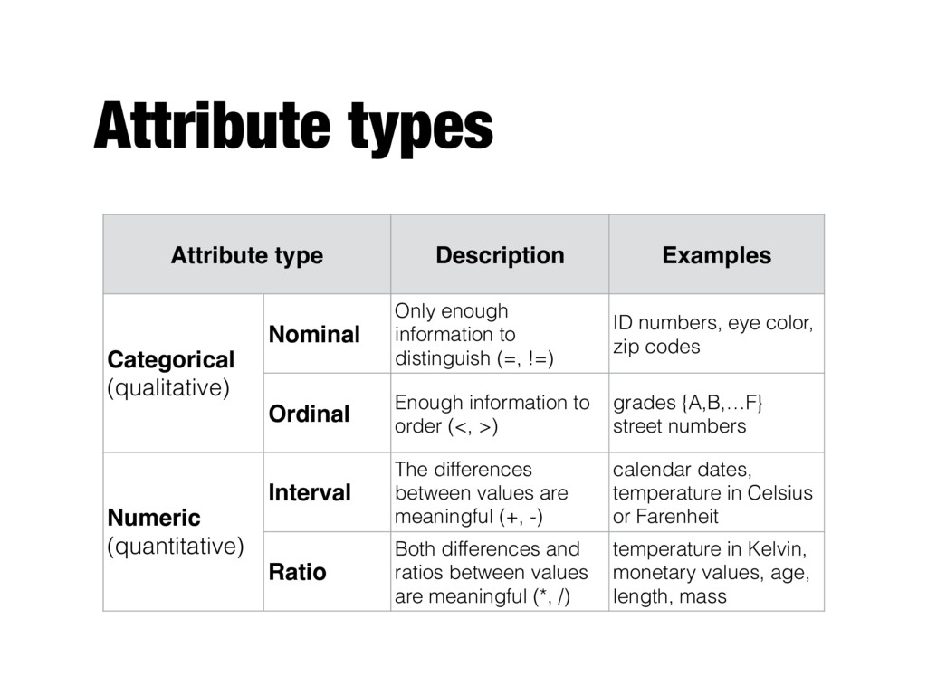
13. Attribute types Attribute type Description Examples Categorical (qualitative) Nominal Only enough information to distinguish (=, !=) ID numbers, eye color, zip codes Ordinal Enough information to order (<, >) grades {A,B,…F}
 street numbers Numeric (quantitative) Interval The differences between values are meaningful (+, -) calendar dates, temperature in Celsius or Farenheit Ratio Both differences and ratios between values are meaningful (*, /) temperature in Kelvin, monetary values, age, length, mass
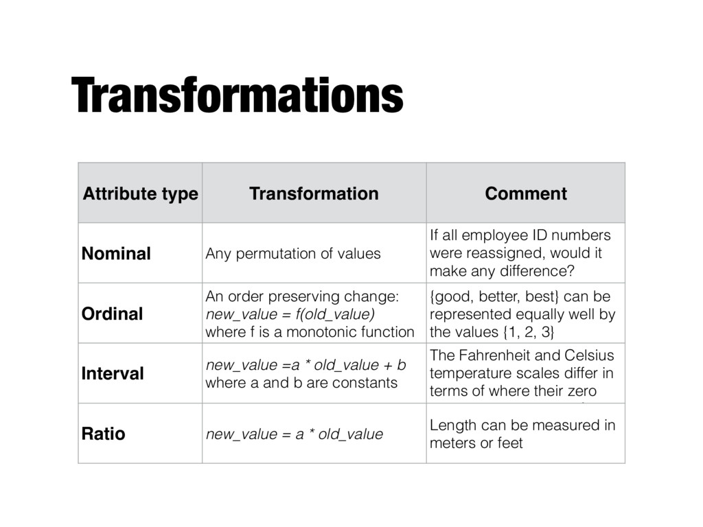
14. Transformations Attribute type Transformation Comment Nominal Any permutation of values If all employee ID numbers were reassigned, would it make any difference? Ordinal An order preserving change:
 new_value = f(old_value) 
 where f is a monotonic function {good, better, best} can be represented equally well by the values {1, 2, 3} Interval new_value =a * old_value + b where a and b are constants The Fahrenheit and Celsius temperature scales differ in terms of where their zero value is and the size of a Ratio new_value = a * old_value Length can be measured in meters or feet
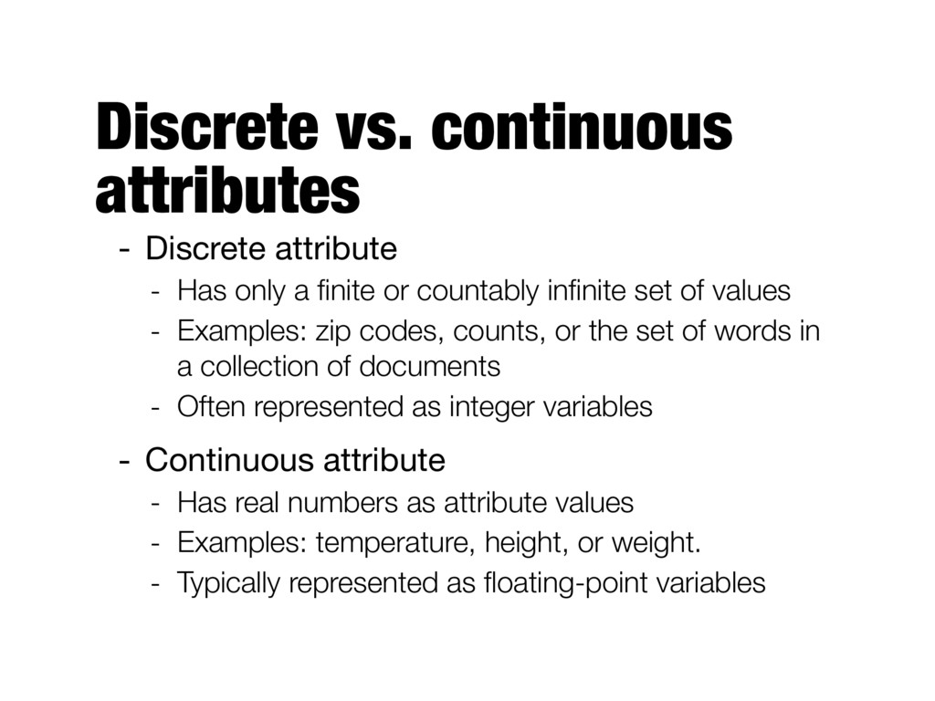
15. Discrete vs. continuous attributes - Discrete attribute - Has only a finite or countably infinite set of values - Examples: zip codes, counts, or the set of words in a collection of documents - Often represented as integer variables - Continuous attribute - Has real numbers as attribute values - Examples: temperature, height, or weight. - Typically represented as floating-point variables
16. Asymmetric attributes - Only presence counts (i.e., only non-zero attribute values) Document 1 season timeout lost wi n game score ball pla y coach team Document 2 Document 3 3 0 5 0 2 6 0 2 0 2 0 0 7 0 2 1 0 0 3 0 0 1 0 0 1 2 2 0 3 0
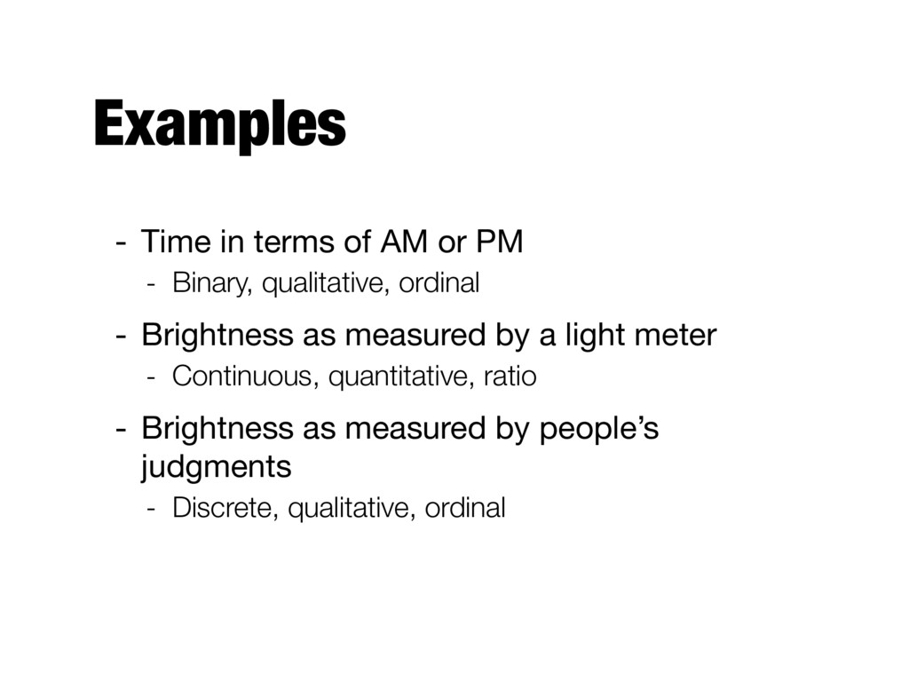
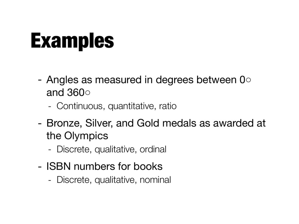
17. Examples - Time in terms of AM or PM - Binary, qualitative, ordinal - Brightness as measured by a light meter - Continuous, quantitative, ratio - Brightness as measured by people’s judgments - Discrete, qualitative, ordinal
18. Examples - Angles as measured in degrees between 0◦ and 360◦ - Continuous, quantitative, ratio - Bronze, Silver, and Gold medals as awarded at the Olympics - Discrete, qualitative, ordinal - ISBN numbers for books - Discrete, qualitative, nominal 

19. Characteristics of Structured Data - Dimensionality - Curse of Dimensionality - Sparsity - Only presence counts - Resolution - Patterns depend on the scale
20. Types of data sets - Record - Data Matrix - Document Data - Transaction Data - Graph - Ordered
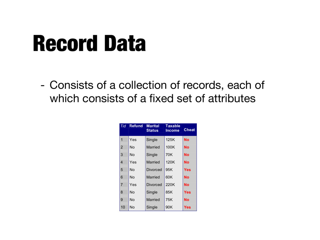
21. Record Data - Consists of a collection of records, each of which consists of a fixed set of attributes Tid Refund Marital Status Taxable Income Cheat 1 Yes Single 125K No 2 No Married 100K No 3 No Single 70K No 4 Yes Married 120K No 5 No Divorced 95K Yes 6 No Married 60K No 7 Yes Divorced 220K No 8 No Single 85K Yes 9 No Married 75K No 10 No Single 90K Yes 10
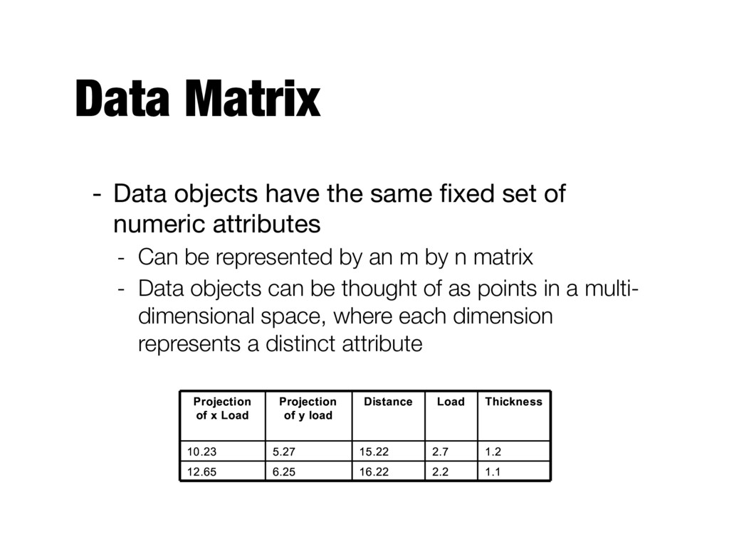
22. Data Matrix - Data objects have the same fixed set of numeric attributes - Can be represented by an m by n matrix - Data objects can be thought of as points in a multi- dimensional space, where each dimension represents a distinct attribute 1.1 2.2 16.22 6.25 12.65 1.2 2.7 15.22 5.27 10.23 Thickness Load Distance Projection of y load Projection of x Load 1.1 2.2 16.22 6.25 12.65 1.2 2.7 15.22 5.27 10.23 Thickness Load Distance Projection of y load Projection of x Load
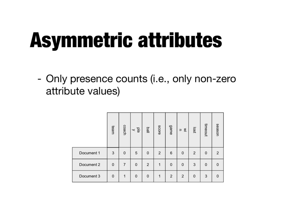
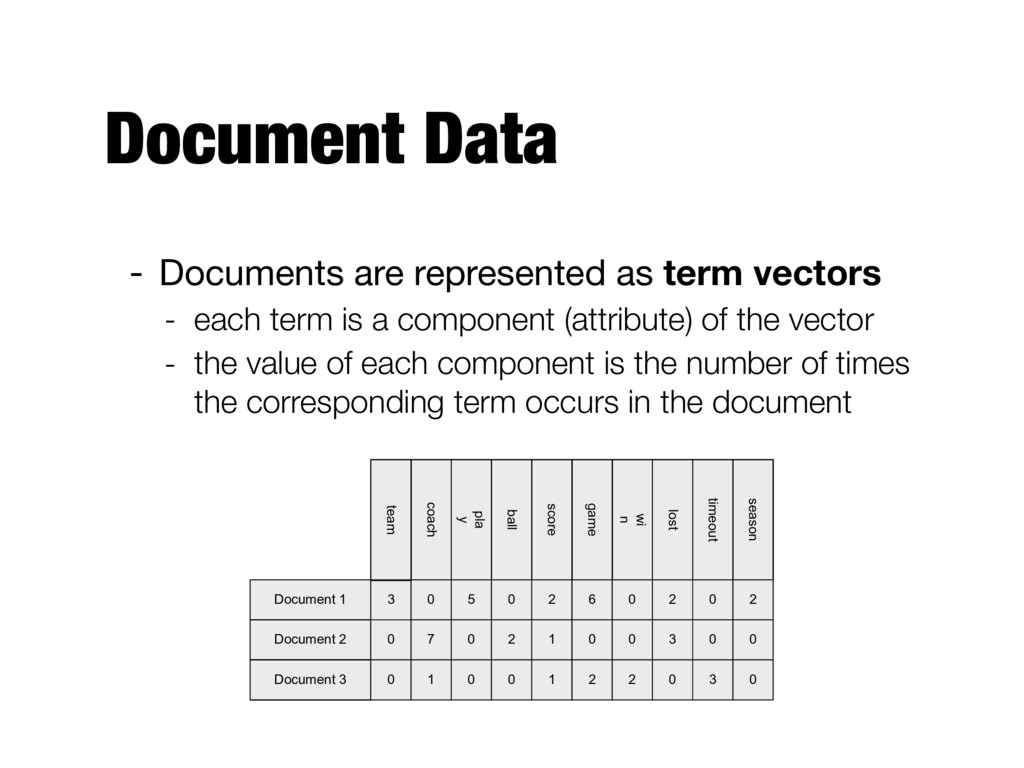
23. Document Data - Documents are represented as term vectors - each term is a component (attribute) of the vector - the value of each component is the number of times the corresponding term occurs in the document Document 1 season timeout lost wi n game score ball pla y coach team Document 2 Document 3 3 0 5 0 2 6 0 2 0 2 0 0 7 0 2 1 0 0 3 0 0 1 0 0 1 2 2 0 3 0
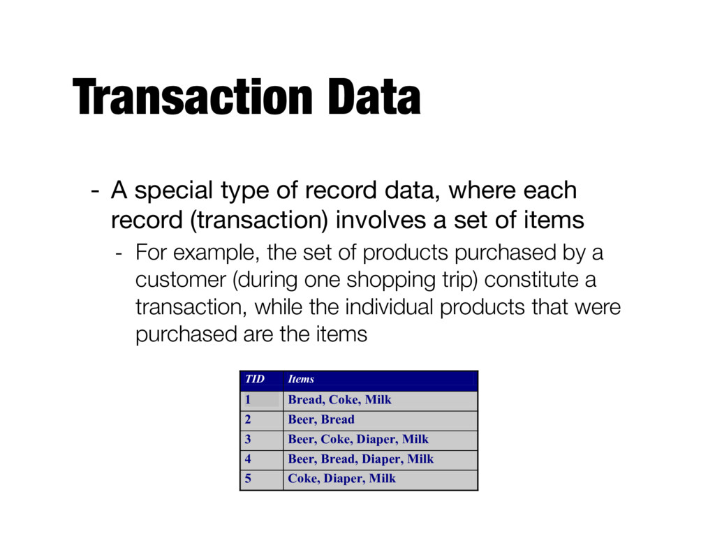
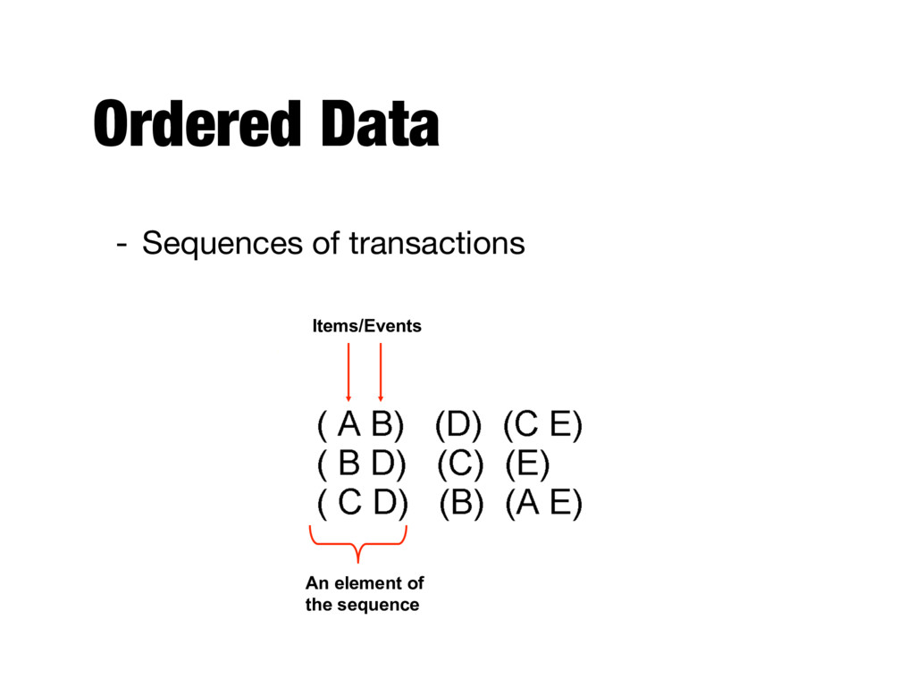
24. Transaction Data - A special type of record data, where each record (transaction) involves a set of items - For example, the set of products purchased by a customer (during one shopping trip) constitute a transaction, while the individual products that were purchased are the items TID Items 1 Bread, Coke, Milk 2 Beer, Bread 3 Beer, Coke, Diaper, Milk 4 Beer, Bread, Diaper, Milk 5 Coke, Diaper, Milk
25. Graph Data - Examples HTML links Chemical data
26. Ordered Data - Sequences of transactions An element of the sequence Items/Events
27. Ordered Data - Genomic sequence data GGTTCCGCCTTCAGCCCCGCGCC CGCAGGGCCCGCCCCGCGCCGTC GAGAAGGGCCCGCCTGGCGGGCG GGGGGAGGCGGGGCCGCCCGAGC CCAACCGAGTCCGACCAGGTGCC CCCTCTGCTCGGCCTAGACCTGA GCTCATTAGGCGGCAGCGGACAG GCCAAGTAGAACACGCGAAGCGC TGGGCTGCCTGCTGCGACCAGGG
28. Ordered Data - Spatio-temporal Data Average Monthly Temperature of land and ocean
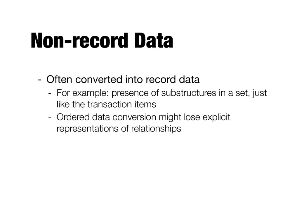
29. Non-record Data - Often converted into record data - For example: presence of substructures in a set, just like the transaction items - Ordered data conversion might lose explicit representations of relationships
30. Data Quality
31. Data Quality Problems - Data won’t be perfect - Human error - Limitations of measuring devices - Flaws in the data collection process - Data is of high quality if it is suitable for its intended use - Much work in data mining focuses on devising robust algorithms that produce acceptable results even when noise is present
32. Typical Data Quality Problems - Noise - Random component of a measurement error - For example, distortion of a person’s voice when talking on a poor phone - Outliers - Data objects with characteristics that are considerably different than most of the other data objects in the data set
33. Typical Data Quality Problems (2) - Missing values - Information is not collected - E.g., people decline to give their age and weight - Attributes may not be applicable to all cases - E.g., annual income is not applicable to children - Solutions - Eliminate an entire object or attribute - Estimate them by neighbor values - Ignore them during analysis
34. Typical Data Quality Problems (3) - Inconsistent data - Data may have some inconsistencies even among present, acceptable values - E.g. Zip code value doesn't correspond to the city value - Duplicate data - Data objects that are duplicates, or almost duplicates of one another - E.g., Same person with multiple email addresses
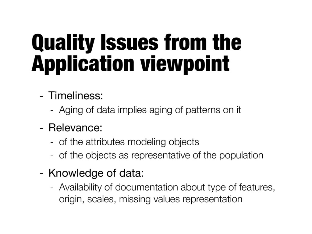
35. Quality Issues from the Application viewpoint - Timeliness: - Aging of data implies aging of patterns on it - Relevance: - of the attributes modeling objects - of the objects as representative of the population - Knowledge of data: - Availability of documentation about type of features, origin, scales, missing values representation
36. Data Preprocessing
37. Data Preprocessing - Different strategies and techniques to make the data more suitable for data mining - Aggregation - Sampling - Dimensionality reduction - Feature subset selection - Feature creation - Discretization and binarization - Attribute transformation
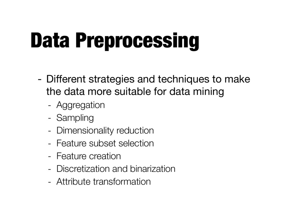
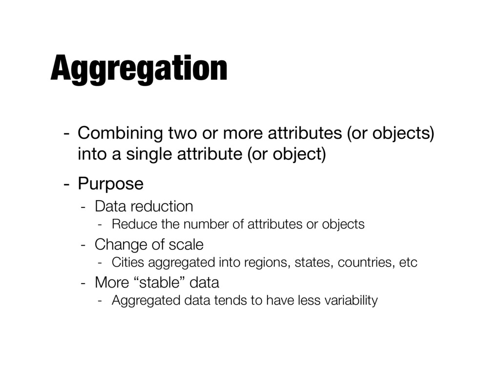
38. Aggregation - Combining two or more attributes (or objects) into a single attribute (or object) - Purpose - Data reduction - Reduce the number of attributes or objects - Change of scale - Cities aggregated into regions, states, countries, etc - More “stable” data - Aggregated data tends to have less variability
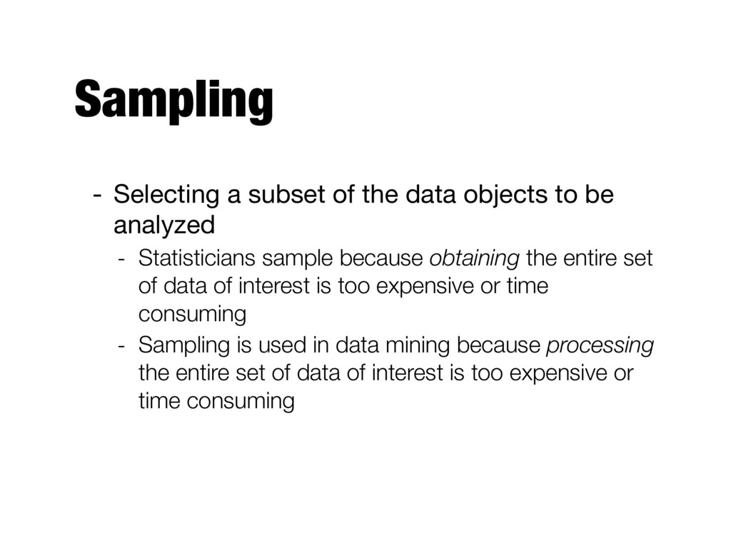
39. Sampling - Selecting a subset of the data objects to be analyzed - Statisticians sample because obtaining the entire set of data of interest is too expensive or time consuming - Sampling is used in data mining because processing the entire set of data of interest is too expensive or time consuming
40. Sampling - A sample is representative if it has approximately the same property (of interest) as the original set of data - Key issues: sampling method and sample size
41. Types of Sampling - Simple random sampling - Any particular item is selected with equal probability - Sampling without replacement - As each item is selected, it is removed from the population - Sampling with replacement - Objects are not removed from the population as they are selected (same object can be picked up more than once) - Stratified sampling - Split the data into several partitions; then draw random samples from each partition
42. Sample size 8000 points 2000 Points 500 Points
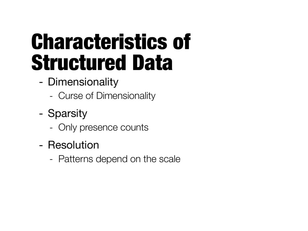
43. Curse of Dimensionality - Many types of data analysis become significantly harder as the dimensionality of the data increases - When dimensionality increases, data becomes increasingly sparse in the space that it occupies - Definitions of density and distance between points become less meaningful
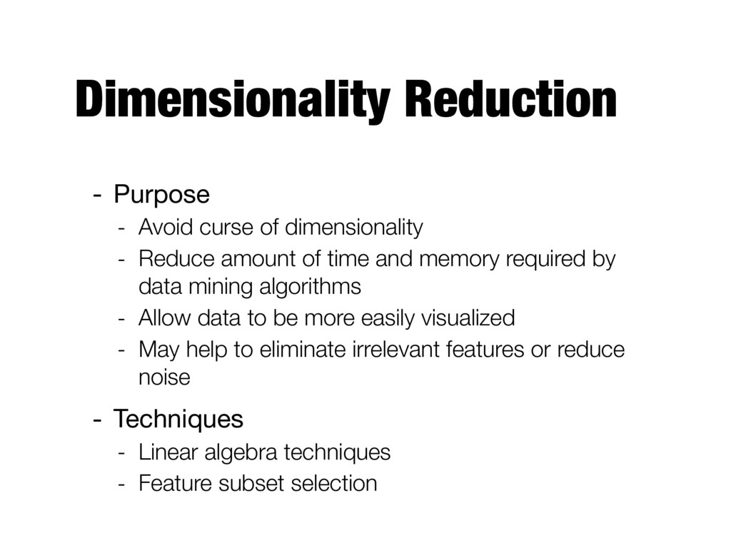
44. Dimensionality Reduction - Purpose - Avoid curse of dimensionality - Reduce amount of time and memory required by data mining algorithms - Allow data to be more easily visualized - May help to eliminate irrelevant features or reduce noise - Techniques - Linear algebra techniques - Feature subset selection
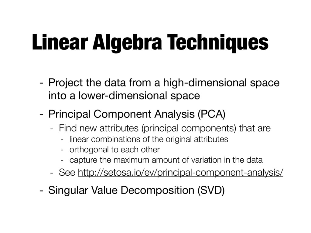
45. Linear Algebra Techniques - Project the data from a high-dimensional space into a lower-dimensional space - Principal Component Analysis (PCA) - Find new attributes (principal components) that are - linear combinations of the original attributes - orthogonal to each other - capture the maximum amount of variation in the data - See http://setosa.io/ev/principal-component-analysis/ - Singular Value Decomposition (SVD)
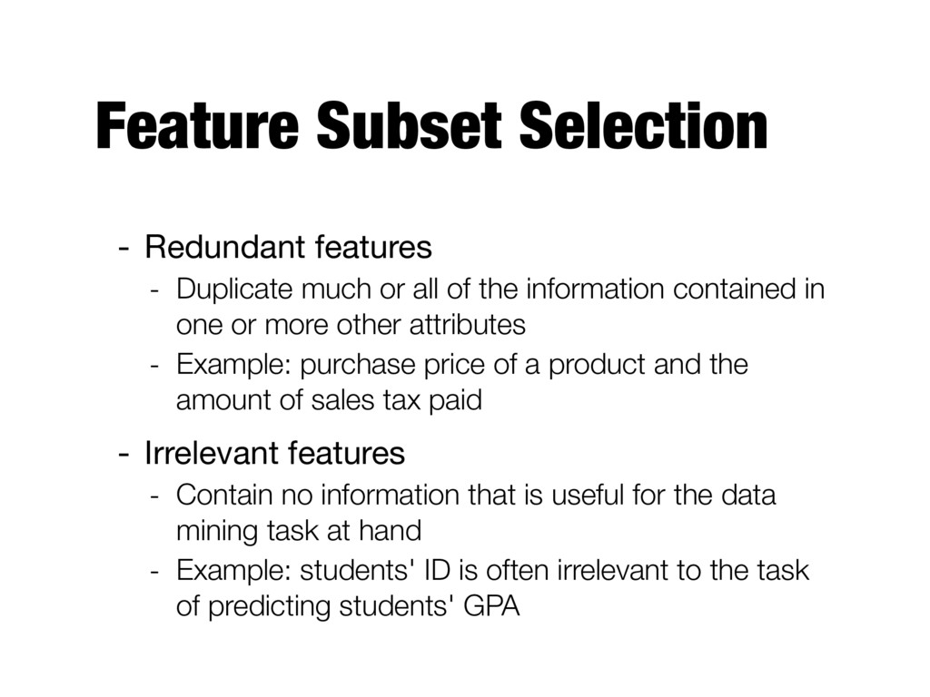
46. Feature Subset Selection - Redundant features - Duplicate much or all of the information contained in one or more other attributes - Example: purchase price of a product and the amount of sales tax paid - Irrelevant features - Contain no information that is useful for the data mining task at hand - Example: students' ID is often irrelevant to the task of predicting students' GPA
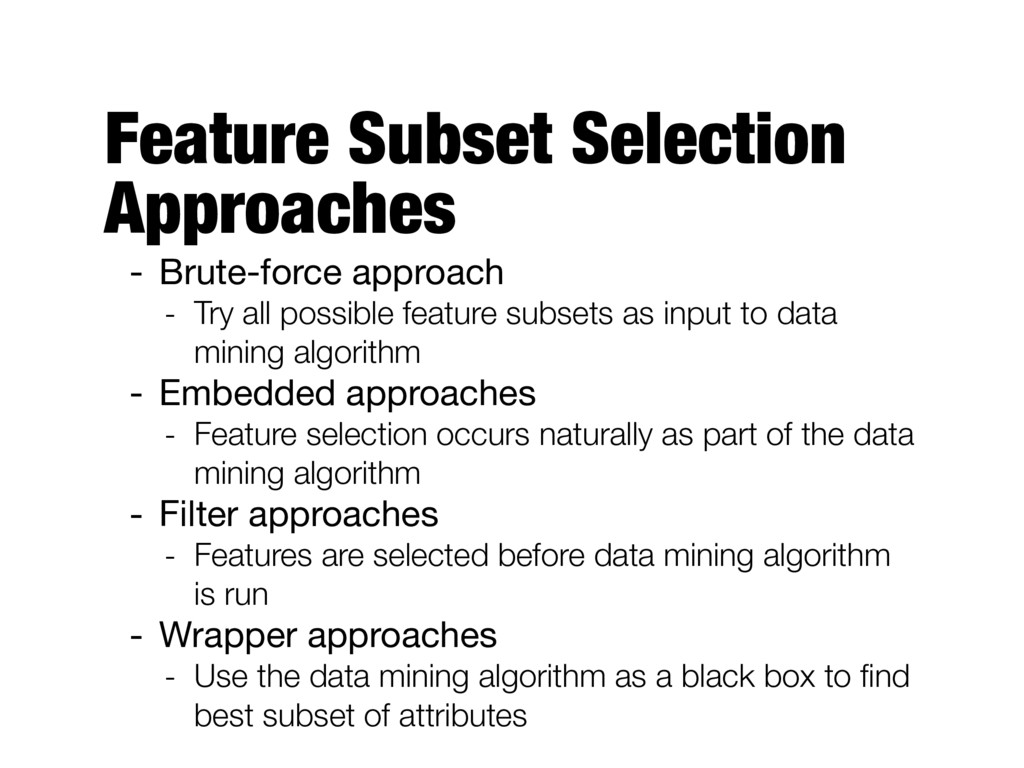
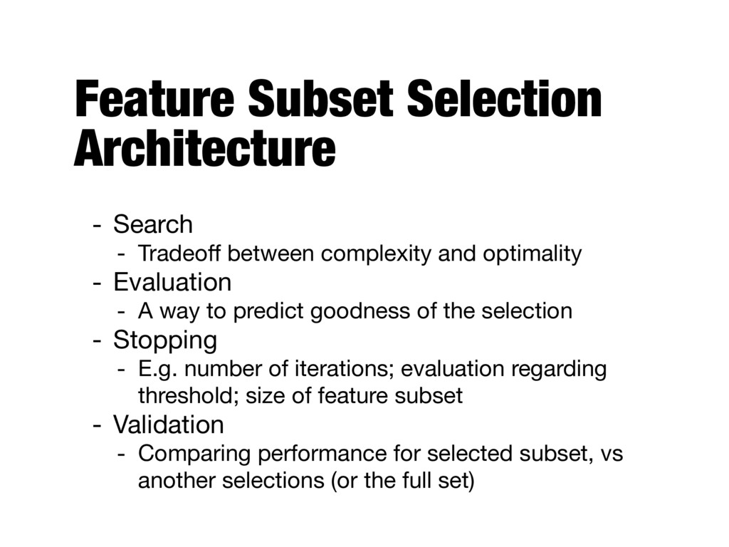
47. Feature Subset Selection Approaches - Brute-force approach - Try all possible feature subsets as input to data mining algorithm - Embedded approaches - Feature selection occurs naturally as part of the data mining algorithm - Filter approaches - Features are selected before data mining algorithm is run - Wrapper approaches - Use the data mining algorithm as a black box to find best subset of attributes
48. Feature Subset Selection Architecture - Search - Tradeoff between complexity and optimality - Evaluation - A way to predict goodness of the selection - Stopping - E.g. number of iterations; evaluation regarding threshold; size of feature subset - Validation - Comparing performance for selected subset, vs another selections (or the full set)
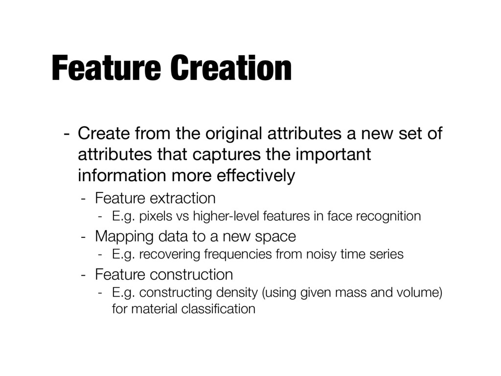
49. Feature Creation - Create from the original attributes a new set of attributes that captures the important information more effectively - Feature extraction - E.g. pixels vs higher-level features in face recognition - Mapping data to a new space - E.g. recovering frequencies from noisy time series - Feature construction - E.g. constructing density (using given mass and volume) for material classification
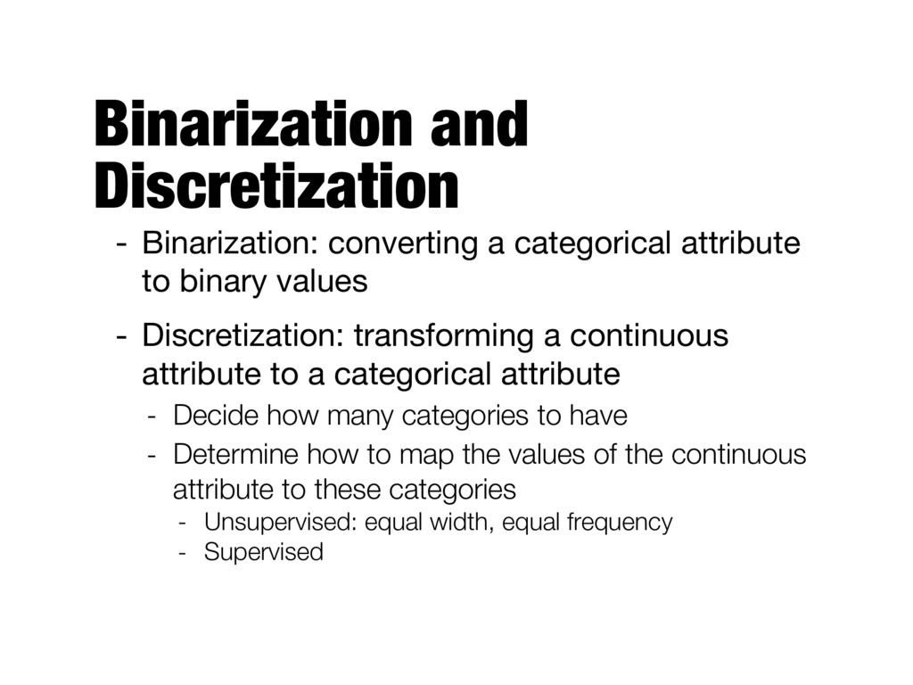
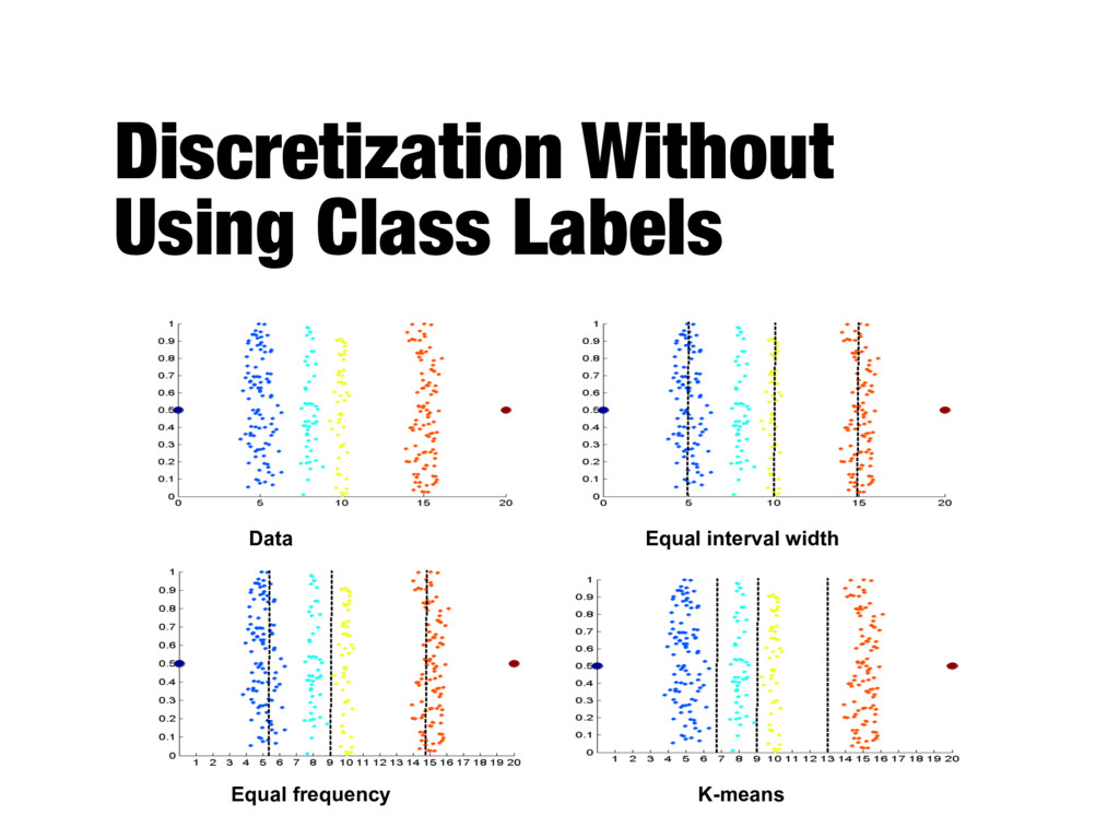
50. Binarization and Discretization - Binarization: converting a categorical attribute to binary values - Discretization: transforming a continuous attribute to a categorical attribute - Decide how many categories to have - Determine how to map the values of the continuous attribute to these categories - Unsupervised: equal width, equal frequency - Supervised
51. Discretization Without Using Class Labels Data Equal interval width Equal frequency K-means
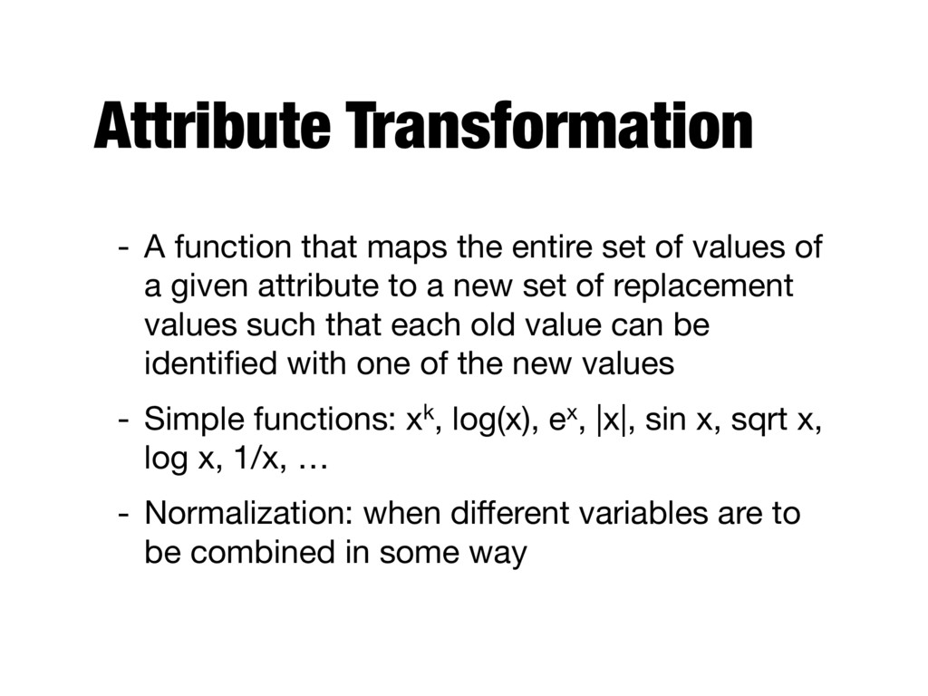
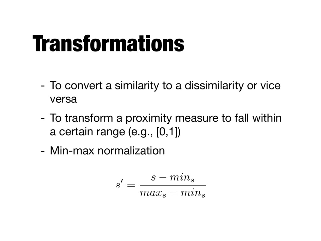
52. Attribute Transformation - A function that maps the entire set of values of a given attribute to a new set of replacement values such that each old value can be identified with one of the new values - Simple functions: xk, log(x), ex, |x|, sin x, sqrt x, log x, 1/x, … - Normalization: when different variables are to be combined in some way
53. Proximity Measures
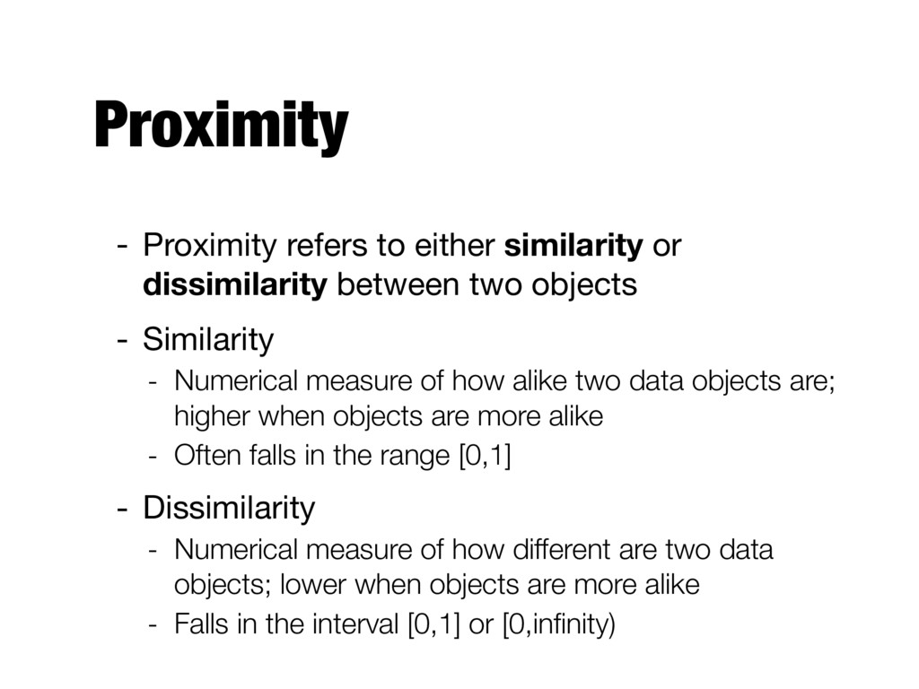
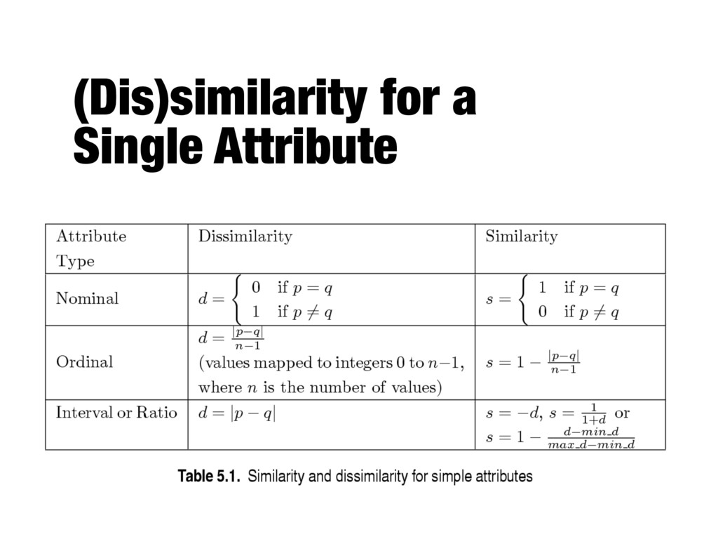
54. Proximity - Proximity refers to either similarity or dissimilarity between two objects - Similarity - Numerical measure of how alike two data objects are; higher when objects are more alike - Often falls in the range [0,1] - Dissimilarity - Numerical measure of how different are two data objects; lower when objects are more alike - Falls in the interval [0,1] or [0,infinity)
55. Transformations - To convert a similarity to a dissimilarity or vice versa - To transform a proximity measure to fall within a certain range (e.g., [0,1]) - Min-max normalization s 0 = s mins maxs mins
56. (Dis)similarity for a 
 Single Attribute
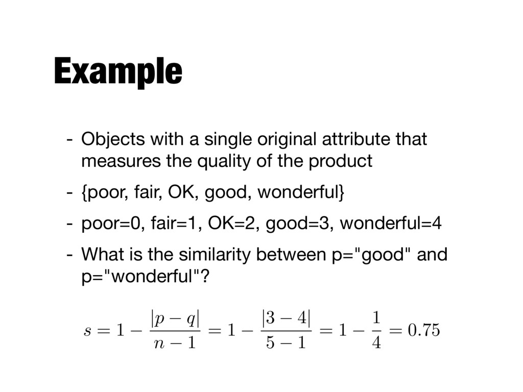
57. Example - Objects with a single original attribute that measures the quality of the product - {poor, fair, OK, good, wonderful} - poor=0, fair=1, OK=2, good=3, wonderful=4 - What is the similarity between p="good" and p="wonderful"? s = 1 |p q| n 1 = 1 |3 4| 5 1 = 1 1 4 = 0.75
58. Dissimilarities between 
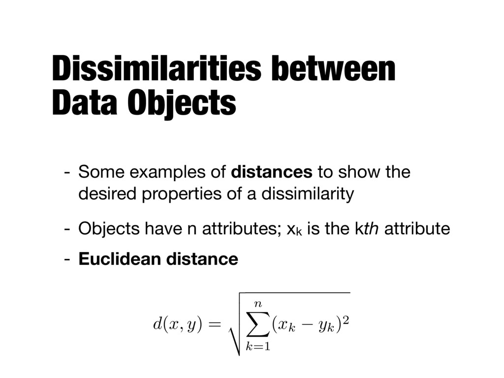
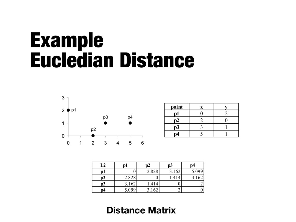
 Data Objects - Objects have n attributes; xk is the kth attribute - Euclidean distance d ( x, y ) = v u u t n X k=1 ( xk yk)2 - Some examples of distances to show the desired properties of a dissimilarity
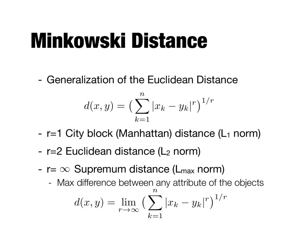
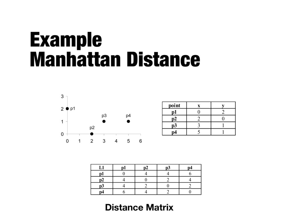
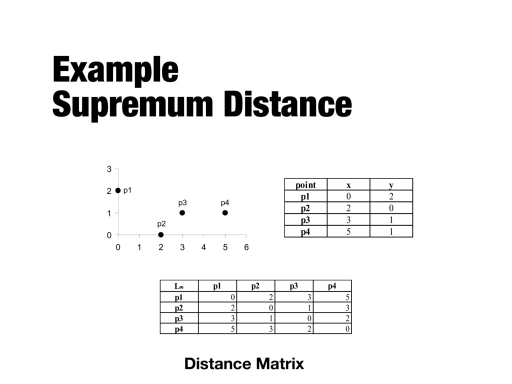
59. Minkowski Distance - Generalization of the Euclidean Distance - r=1 City block (Manhattan) distance (L1 norm) - r=2 Euclidean distance (L2 norm) - r= Supremum distance (Lmax norm) - Max difference between any attribute of the objects d ( x, y ) = n X k=1 | xk yk |r 1/r 1 d ( x, y ) = lim r!1 n X k=1 | xk yk |r 1/r
60. Example 
 Eucledian Distance 0 1 2 3 0 1 2 3 4 5 6 p1 p2 p3 p4 point x y p1 0 2 p2 2 0 p3 3 1 p4 5 1 Distance Matrix p1 p2 p3 p4 p1 0 2.828 3.162 5.099 p2 2.828 0 1.414 3.162 p3 3.162 1.414 0 2 p4 5.099 3.162 2 0 Distance Matrix L2 p1 p2 p3 p4 p1 0 2.828 3.162 5.099 p2 2.828 0 1.414 3.162 p3 3.162 1.414 0 2 p4 5.099 3.162 2 0
61. Example 
 Manhattan Distance 0 1 2 3 0 1 2 3 4 5 6 p1 p2 p3 p4 point x y p1 0 2 p2 2 0 p3 3 1 p4 5 1 Distance Matrix p1 p2 p3 p4 p1 0 2.828 3.162 5.099 p2 2.828 0 1.414 3.162 p3 3.162 1.414 0 2 p4 5.099 3.162 2 0 L1 p1 p2 p3 p4 p1 0 4 4 6 p2 4 0 2 4 p3 4 2 0 2 p4 6 4 2 0 Distance Matrix
62. Example 
 Supremum Distance 0 1 2 3 0 1 2 3 4 5 6 p1 p2 p3 p4 point x y p1 0 2 p2 2 0 p3 3 1 p4 5 1 Distance Matrix p1 p2 p3 p4 p1 0 2.828 3.162 5.099 p2 2.828 0 1.414 3.162 p3 3.162 1.414 0 2 p4 5.099 3.162 2 0 Distance Matrix L∞ p1 p2 p3 p4 p1 0 2 3 5 p2 2 0 1 3 p3 3 1 0 2 p4 5 3 2 0
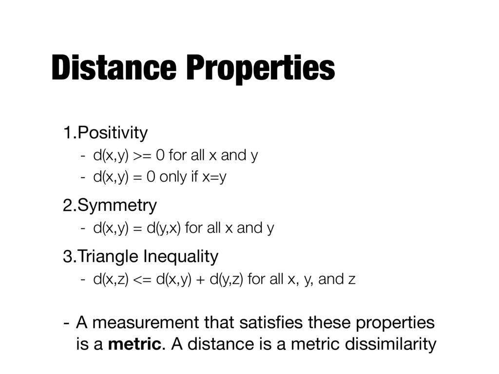
63. Distance Properties 1.Positivity - d(x,y) >= 0 for all x and y - d(x,y) = 0 only if x=y 2.Symmetry - d(x,y) = d(y,x) for all x and y 3.Triangle Inequality - d(x,z) <= d(x,y) + d(y,z) for all x, y, and z - A measurement that satisfies these properties is a metric. A distance is a metric dissimilarity
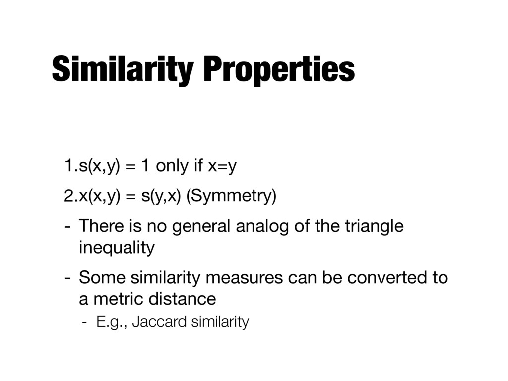
64. Similarity Properties 1.s(x,y) = 1 only if x=y 2.x(x,y) = s(y,x) (Symmetry) - There is no general analog of the triangle inequality - Some similarity measures can be converted to a metric distance - E.g., Jaccard similarity
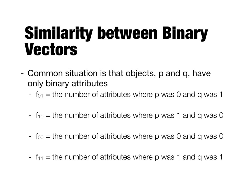
65. Similarity between Binary Vectors - Common situation is that objects, p and q, have only binary attributes - f01 = the number of attributes where p was 0 and q was 1 - f10 = the number of attributes where p was 1 and q was 0 - f00 = the number of attributes where p was 0 and q was 0 - f11 = the number of attributes where p was 1 and q was 1
66. Similarity between Binary Vectors - Simple Matching Coefficient - number of matching attribute values divided by the number of attributes - Jaccard Coefficient - Ignore 0-0 matches SMC = f11 + f00 f01 + f10 + f11 + f00 J = f11 f01 + f10 + f11
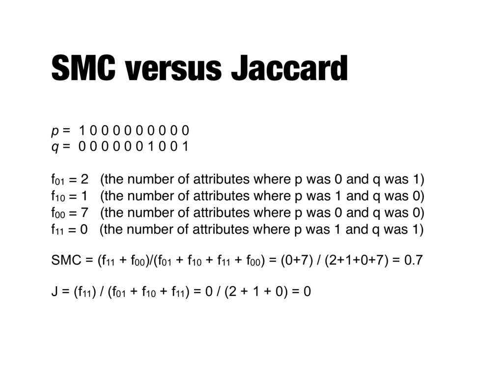
67. SMC versus Jaccard p = 1 0 0 0 0 0 0 0 0 0 q = 0 0 0 0 0 0 1 0 0 1 f01 = 2 (the number of attributes where p was 0 and q was 1) f10 = 1 (the number of attributes where p was 1 and q was 0) f00 = 7 (the number of attributes where p was 0 and q was 0) f11 = 0 (the number of attributes where p was 1 and q was 1) SMC = (f11 + f00)/(f01 + f10 + f11 + f00) = (0+7) / (2+1+0+7) = 0.7 J = (f11) / (f01 + f10 + f11) = 0 / (2 + 1 + 0) = 0
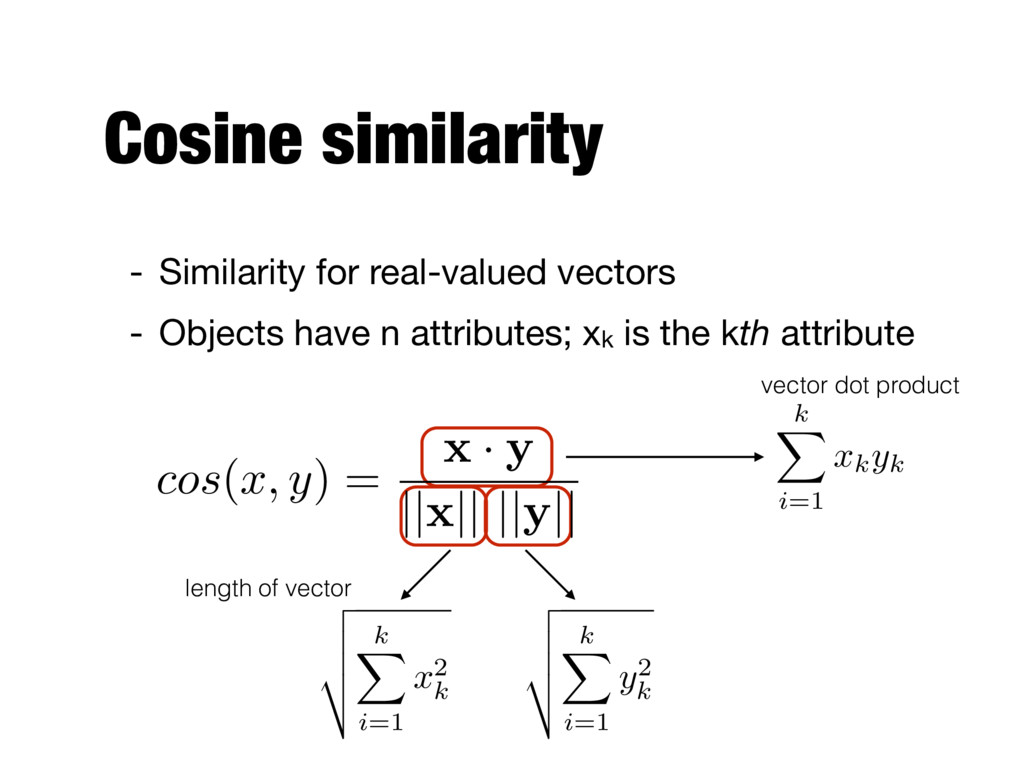
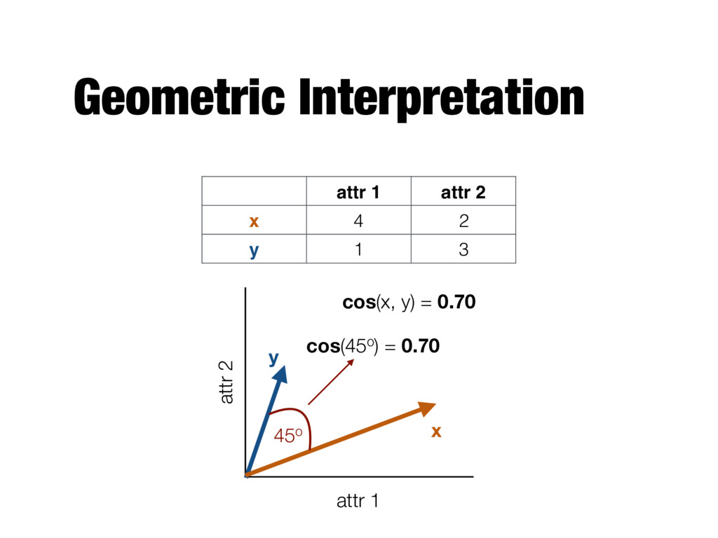
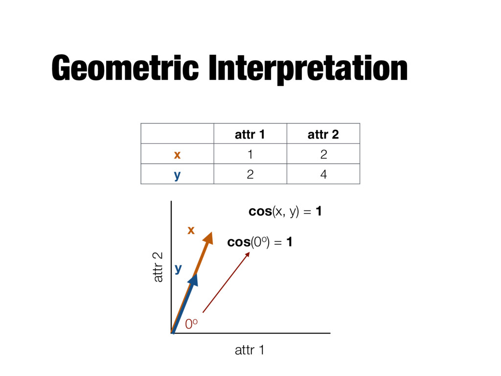
68. Cosine similarity - Similarity for real-valued vectors - Objects have n attributes; xk is the kth attribute cos ( x, y ) = x · y || x || || y || k X i=1 xkyk vector dot product length of vector v u u t k X i=1 x 2 k v u u t k X i=1 y2 k
69. Example attr 1 attr 2 attr 3 attr 4 attr 5 x 1 0 1 0 3 y 0 2 4 0 1 cos ( x, y ) = x · y || x || || y || k X i=1 xkyk v u u t k X i=1 x 2 k v u u t k X i=1 y2 k
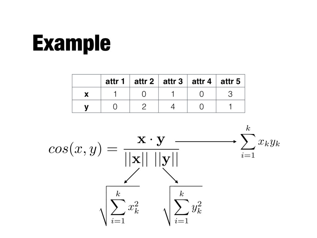
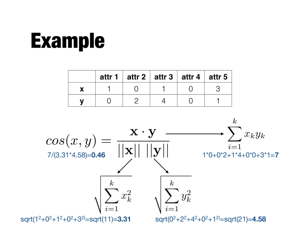
70. Example attr 1 attr 2 attr 3 attr 4 attr 5 x 1 0 1 0 3 y 0 2 4 0 1 cos ( x, y ) = x · y || x || || y || k X i=1 xkyk v u u t k X i=1 x 2 k v u u t k X i=1 y2 k 1*0+0*2+1*4+0*0+3*1=7 sqrt(12+02+12+02+32)=sqrt(11)=3.31 sqrt(02+22+42+02+12)=sqrt(21)=4.58 7/(3.31*4.58)=0.46
71. Geometric Interpretation attr 1 attr 2 x 1 0 y 0 2 attr 1 attr 2 x cos(x, y) = 0 90o cos(90o) = 0 y
72. Geometric Interpretation attr 1 attr 2 x 4 2 y 1 3 attr 1 attr 2 y x cos(x, y) = 0.70 45o cos(45o) = 0.70
73. Geometric Interpretation attr 1 attr 2 x 1 2 y 2 4 attr 1 attr 2 y x cos(x, y) = 1 0o cos(0o) = 1