Effect of inter annual and seasonal variability on oil fate along the Texas coastline

Presentation at the Estuarine and Coastal Modeling conference in San Diego, CA, November 4-6, 2014.

Transcript

1. Effect of Interannual and Seasonal Variability on Oil Fate along the Texas Coastline Kristen Thyng Rob Hetland ECM 2013 Texas A&M University November 4, 2013 Kristen Thyng (Texas A&M) ECM 2013 November 4, 2013 1 / 16
2. Overview Using particle tracking Visualize Lagrangian flow TRACMASS Conserves mass Can track forward and backward and get the same paths TracPy: TRACMASS now wrapped in Python Applied here to cross-shelf transport - controls what material can reach shoreline Kristen Thyng (Texas A&M) ECM 2013 November 4, 2013 2 / 16
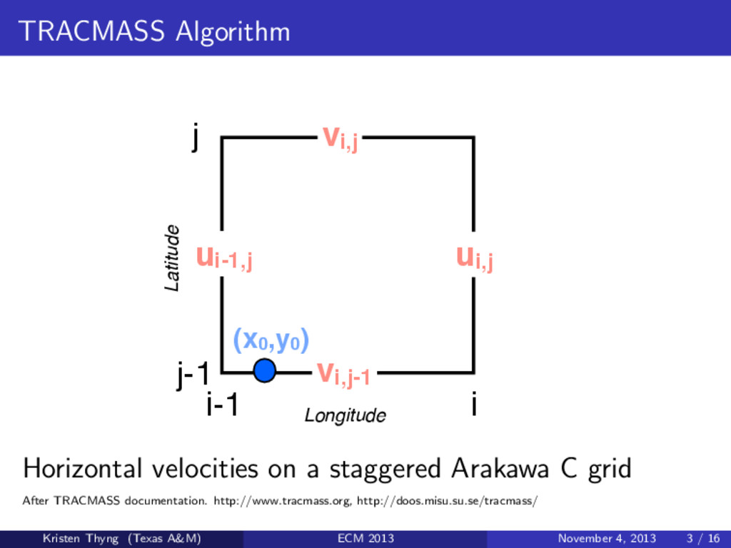
3. TRACMASS Algorithm j j-1 i-1 i ui,j ui-1,j vi,j vi,j-1 (x0,y0 ) Longitude Latitude u(x) Horizontal velocities on a staggered Arakawa C grid After TRACMASS documentation. http://www.tracmass.org, http://doos.misu.su.se/tracmass/ Kristen Thyng (Texas A&M) ECM 2013 November 4, 2013 3 / 16
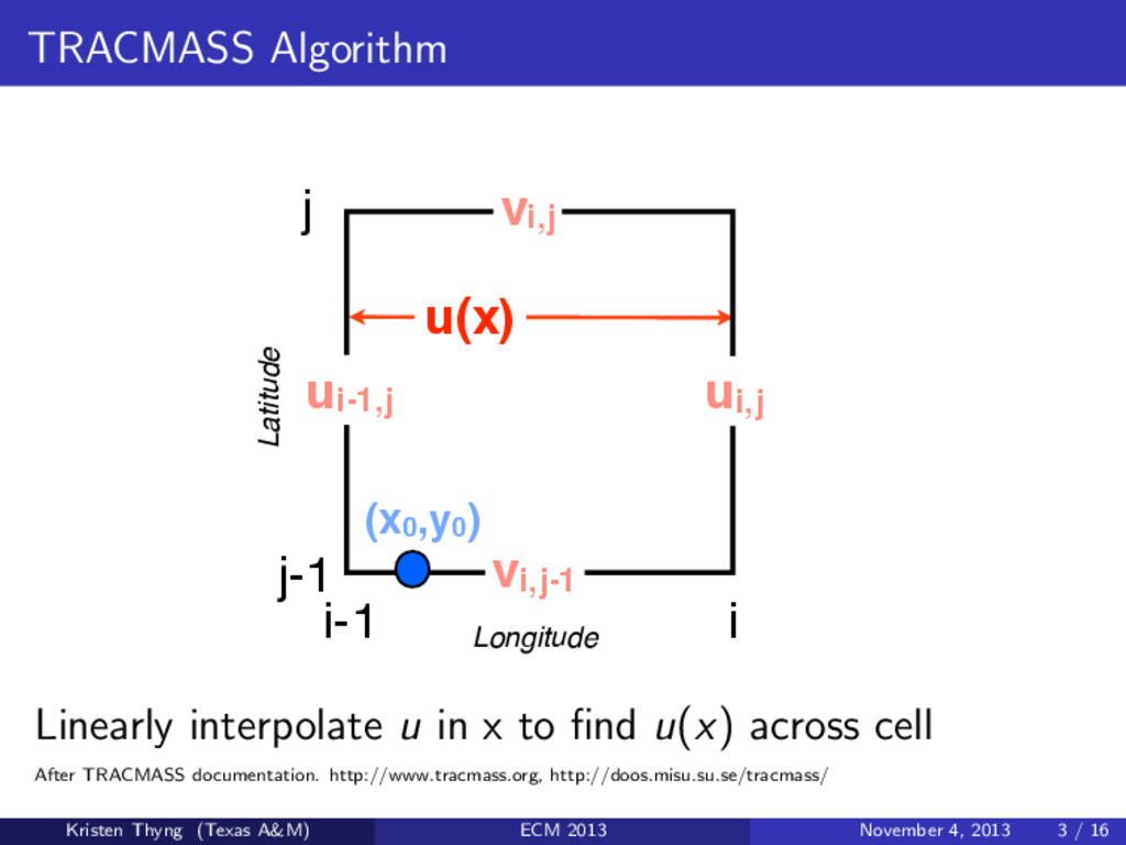
4. TRACMASS Algorithm j j-1 i-1 i ui,j ui-1,j vi,j vi,j-1 (x0,y0 ) Longitude Latitude u(x) Linearly interpolate u in x to find u(x) across cell After TRACMASS documentation. http://www.tracmass.org, http://doos.misu.su.se/tracmass/ Kristen Thyng (Texas A&M) ECM 2013 November 4, 2013 3 / 16
5. TRACMASS Algorithm j j-1 i-1 i ui,j ui-1,j vi,j vi,j-1 (x0,y0 ) Longitude Latitude dx/dt u(x) u = dx dt After TRACMASS documentation. http://www.tracmass.org, http://doos.misu.su.se/tracmass/ Kristen Thyng (Texas A&M) ECM 2013 November 4, 2013 3 / 16
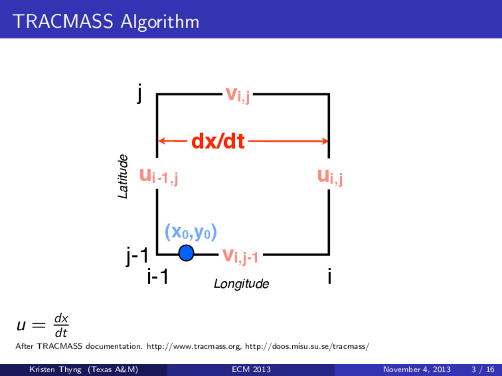
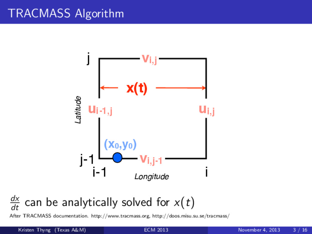
6. TRACMASS Algorithm j j-1 i-1 i ui,j ui-1,j vi,j vi,j-1 (x0,y0 ) Longitude Latitude x(t) u(x) dx/dt dx dt can be analytically solved for x(t) After TRACMASS documentation. http://www.tracmass.org, http://doos.misu.su.se/tracmass/ Kristen Thyng (Texas A&M) ECM 2013 November 4, 2013 3 / 16
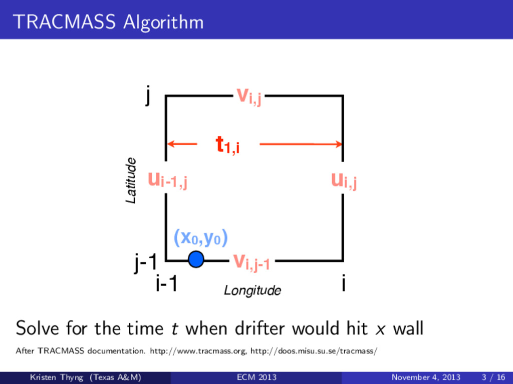
7. TRACMASS Algorithm j j-1 i-1 i ui,j ui-1,j vi,j vi,j-1 (x0,y0 ) Longitude Latitude t1,i u(x) dx/dt x(t) Solve for the time t when drifter would hit x wall After TRACMASS documentation. http://www.tracmass.org, http://doos.misu.su.se/tracmass/ Kristen Thyng (Texas A&M) ECM 2013 November 4, 2013 3 / 16
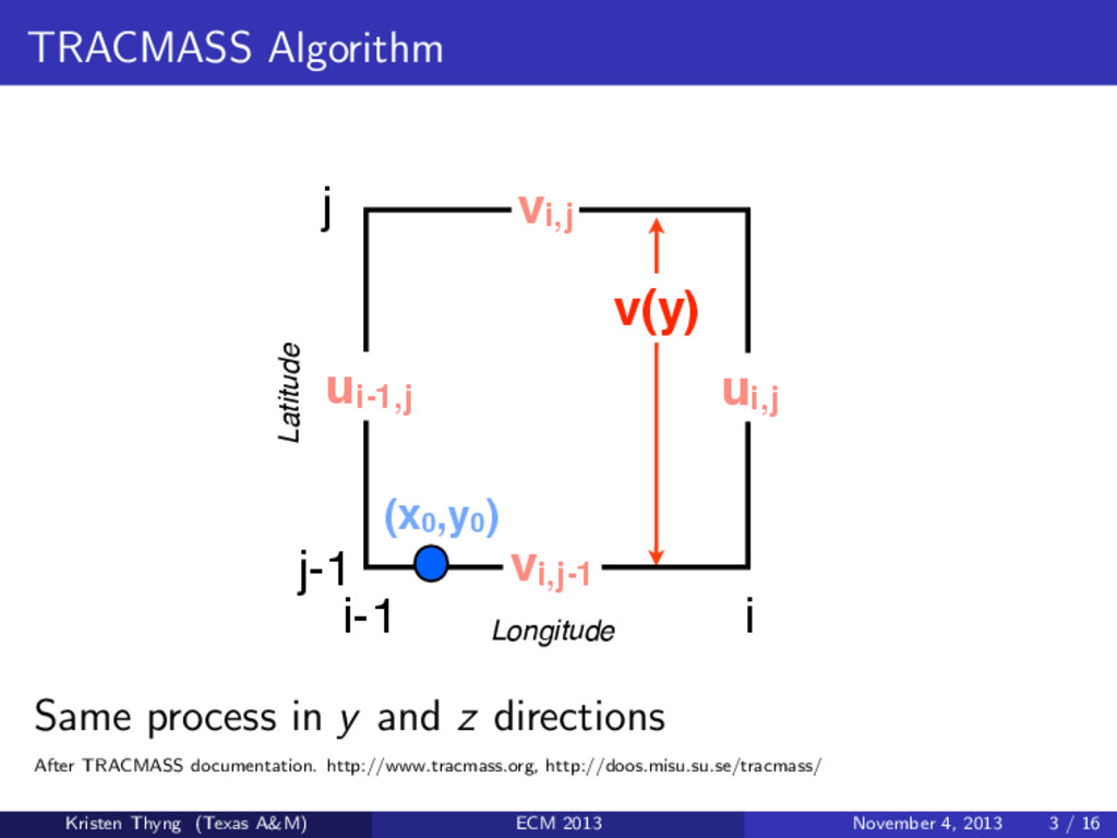
8. TRACMASS Algorithm j j-1 i-1 i ui,j ui-1,j vi,j vi,j-1 (x0,y0 ) Longitude Latitude v(y) Same process in y and z directions After TRACMASS documentation. http://www.tracmass.org, http://doos.misu.su.se/tracmass/ Kristen Thyng (Texas A&M) ECM 2013 November 4, 2013 3 / 16
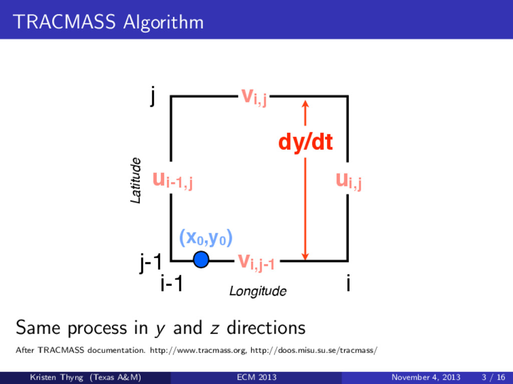
9. TRACMASS Algorithm j j-1 i-1 i ui,j ui-1,j vi,j vi,j-1 (x0,y0 ) Longitude Latitude dy/dt Same process in y and z directions After TRACMASS documentation. http://www.tracmass.org, http://doos.misu.su.se/tracmass/ Kristen Thyng (Texas A&M) ECM 2013 November 4, 2013 3 / 16
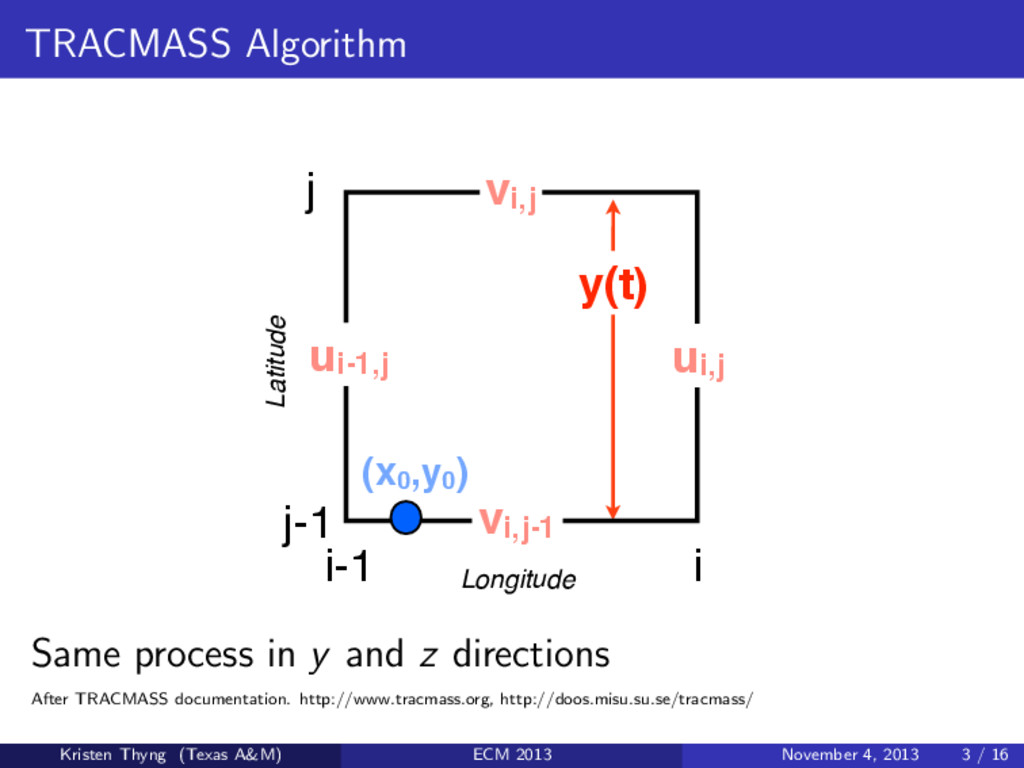
10. TRACMASS Algorithm j j-1 i-1 i ui,j ui-1,j vi,j vi,j-1 (x0,y0 ) Longitude Latitude y(t) Same process in y and z directions After TRACMASS documentation. http://www.tracmass.org, http://doos.misu.su.se/tracmass/ Kristen Thyng (Texas A&M) ECM 2013 November 4, 2013 3 / 16
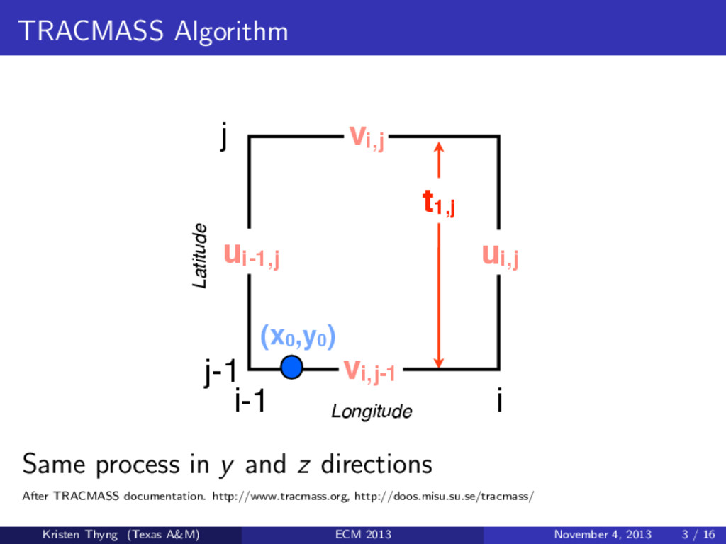
11. TRACMASS Algorithm j j-1 i-1 i ui,j ui-1,j vi,j vi,j-1 (x0,y0 ) Longitude Latitude t1,j Same process in y and z directions After TRACMASS documentation. http://www.tracmass.org, http://doos.misu.su.se/tracmass/ Kristen Thyng (Texas A&M) ECM 2013 November 4, 2013 3 / 16
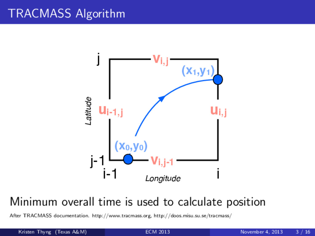
12. TRACMASS Algorithm j j-1 i-1 i ui,j ui-1,j vi,j vi,j-1 (x0,y0 ) Longitude Latitude (x1,y1 ) Minimum overall time is used to calculate position After TRACMASS documentation. http://www.tracmass.org, http://doos.misu.su.se/tracmass/ Kristen Thyng (Texas A&M) ECM 2013 November 4, 2013 3 / 16
13. TRACMASS Algorithm j j-1 i-1 i Ui,j Ui-1,j Vi,j Vi,j-1 (x0,y0 ) Longitude Latitude (x1,y1 ) Instead of velocities, use fluxes to allow for differences in grid sizing After TRACMASS documentation. http://www.tracmass.org, http://doos.misu.su.se/tracmass/ Kristen Thyng (Texas A&M) ECM 2013 November 4, 2013 3 / 16
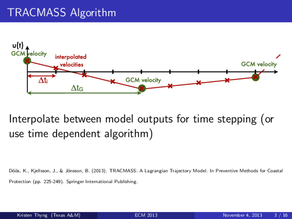
14. TRACMASS Algorithm 7 TRACMASS—A Lagrangian Trajectory Model 235 Fig. 7.6 Schematic illustration of how the velocity fields u(t) can be updated in time, with new GCM data at regular intervals tG in green and linearly interpolated velocity points in red with the time step ti . The number of intermediate time steps between two GCM velocities is in this example IS = tG/ ti = 4 updated successively as new fields are available. If this is made ‘on-line’, i.e., in the same time as the GCM is integrated, then this time interval will simply be the same as the time step the GCM is integrated with, which is typically of the order of minutes in a global GCM. If instead the trajectories are calculated ‘off-line’ it will be at least as often as the fields have been stored by the GCM. A linear time interpolation of the velocity fields between two GCM velocity fields enables a simple way to have shorter time steps by which the fields are updated in Interpolate between model outputs for time stepping (or use time dependent algorithm) D¨ o¨ os, K., Kjellsson, J., & J¨ onsson, B. (2013). TRACMASS: A Lagrangian Trajectory Model. In Preventive Methods for Coastal Protection (pp. 225-249). Springer International Publishing. Kristen Thyng (Texas A&M) ECM 2013 November 4, 2013 3 / 16
15. Validation: inertial oscillation D¨ o¨ os, K., Kjellsson, J., & J¨ onsson, B. (2013). TRACMASS: A Lagrangian Trajectory Model. In Preventive Methods for Coastal Protection (pp. 225-249). Springer International Publishing. Kristen Thyng (Texas A&M) ECM 2013 November 4, 2013 4 / 16
16. TRACMASS Features Subgrid parameterization using: –random turbulent velocities j j-1 i-1 i ui,j+u’ ui-1,j+u’ vi,j+v’ vi,j-1+v’ (x0,y0) Longitude Latitude (x1,y1) (x1,y1)’ After TRACMASS documentation. http://www.tracmass.org, http://doos.misu.su.se/tracmass/ Kristen Thyng (Texas A&M) ECM 2013 November 4, 2013 5 / 16
17. TRACMASS Features Subgrid parameterization using: –random displacement on a circle j j-1 i-1 i ui,j ui-1,j vi,j vi,j-1 (x0,y0) Longitude Latitude (x1,y1) (x1,y1)’ After TRACMASS documentation. http://www.tracmass.org, http://doos.misu.su.se/tracmass/ Kristen Thyng (Texas A&M) ECM 2013 November 4, 2013 5 / 16
18. TRACMASS Features Subgrid parameterization using: –random displacement on an ellipse aligned with isobaths j j-1 i-1 i ui,j ui-1,j vi,j vi,j-1 (x0,y0) Longitude Latitude (x1,y1) (x1,y1)’ After TRACMASS documentation. http://www.tracmass.org, http://doos.misu.su.se/tracmass/ Kristen Thyng (Texas A&M) ECM 2013 November 4, 2013 5 / 16
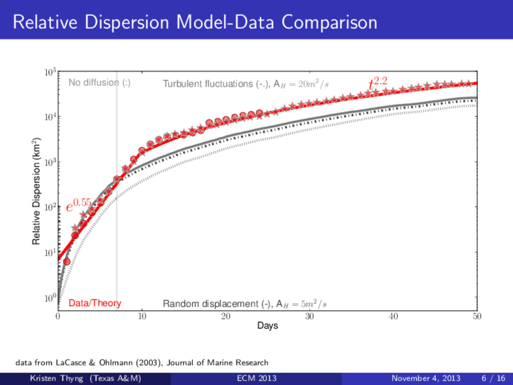
19. Relative Dispersion Model-Data Comparison 0 10 20 30 40 50 Days 100 101 102 103 104 105 Relative Dispersion (km2) Data/Theory No diffusion (:) Turbulent fluctuations (-.), A H = 20m2/s Random displacement (-), A H = 5m2/s e0.55 t2.2 data from LaCasce & Ohlmann (2003), Journal of Marine Research Kristen Thyng (Texas A&M) ECM 2013 November 4, 2013 6 / 16
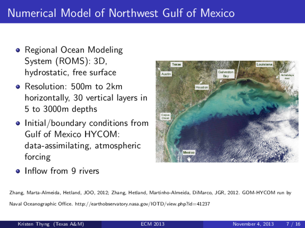
20. Numerical Model of Northwest Gulf of Mexico Regional Ocean Modeling System (ROMS): 3D, hydrostatic, free surface Resolution: 500m to 2km horizontally, 30 vertical layers in 5 to 3000m depths Initial/boundary conditions from Gulf of Mexico HYCOM: data-assimilating, atmospheric forcing Inflow from 9 rivers Mexico Galveston Bay Atchafalaya river Corpus Christi Houston Louisiana Texas Austin Zhang, Marta-Almeida, Hetland, JOO, 2012; Zhang, Hetland, Martinho-Almeida, DiMarco, JGR, 2012. GOM-HYCOM run by Naval Oceanographic Office. http://earthobservatory.nasa.gov/IOTD/view.php?id=41237 Kristen Thyng (Texas A&M) ECM 2013 November 4, 2013 7 / 16
21. Transport Mass-conserving formulation allows use of drifters to calculate transport and flux Kristen Thyng (Texas A&M) ECM 2013 November 4, 2013 8 / 16
22. Drifter Simulations Kristen Thyng (Texas A&M) ECM 2013 November 4, 2013 9 / 16
23. Cross-shelf Connectivity: Seasonality Kristen Thyng (Texas A&M) ECM 2013 November 4, 2013 10 / 16
24. Cross-shelf Connectivity: Seasonality, Area 1 Kristen Thyng (Texas A&M) ECM 2013 November 4, 2013 11 / 16
25. Cross-shelf Connectivity: Seasonality, Area 1 Mississippi outflow consistently causes cross-shelf transport Kristen Thyng (Texas A&M) ECM 2013 November 4, 2013 11 / 16
26. Cross-shelf Connectivity: Seasonality, Area 2 Kristen Thyng (Texas A&M) ECM 2013 November 4, 2013 12 / 16
27. Cross-shelf Connectivity: Seasonality, Area 2 (a) February 2005 (b) July 2006 Loop current eddies do not have a seasonal cycle Kristen Thyng (Texas A&M) ECM 2013 November 4, 2013 12 / 16
28. Cross-shelf Connectivity: Seasonality, Area 3 Kristen Thyng (Texas A&M) ECM 2013 November 4, 2013 13 / 16
29. Cross-shelf Connectivity: Seasonality, Area 3 Mean winds from east-west in non-summer and from west-east in summer Kristen Thyng (Texas A&M) ECM 2013 November 4, 2013 13 / 16
30. Cross-shelf Connectivity: Seasonality, Area 3 Mean winds from east-west in non-summer and from west-east in summer Kristen Thyng (Texas A&M) ECM 2013 November 4, 2013 13 / 16
31. Cross-shelf Connectivity: Seasonality, Area 4 Kristen Thyng (Texas A&M) ECM 2013 November 4, 2013 14 / 16
32. Cross-shelf Connectivity: Seasonality, Area 4 Baroclinic shelf eddies in the summer Rob Hetland, http://pong.tamu.edu/ rob/mch/mayjune/sss 2004.mp4 Kristen Thyng (Texas A&M) ECM 2013 November 4, 2013 14 / 16
33. Cross-shelf Connectivity: Seasonality, Area 4 Baroclinic shelf eddies in the summer Marta-Almeida, Hetland, & Zhang (2013), JGR. Kristen Thyng (Texas A&M) ECM 2013 November 4, 2013 14 / 16
34. Cross-shelf Connectivity: Interannual Variability: Summer Kristen Thyng (Texas A&M) ECM 2013 November 4, 2013 15 / 16
35. Thank you! Kristen Thyng (Texas A&M) ECM 2013 November 4, 2013 16 / 16