Tidal current turbine power capture and impact in an idealized channel simulation

Poster presented at the European Wave and Tidal Energy Conference (EWTEC) in 2013.

Transcript

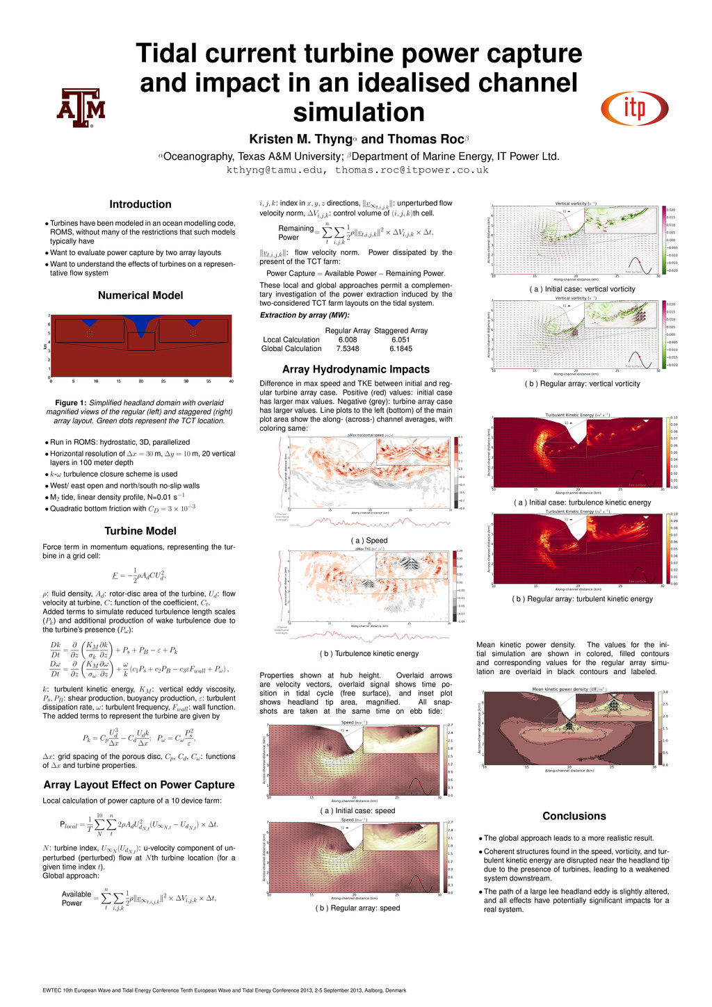
1. Tidal current turbine power capture and impact in an idealised channel simulation Kristen M. Thyngα and Thomas Rocβ αOceanography, Texas A&M University; βDepartment of Marine Energy, IT Power Ltd. kthyng@tamu.edu, thomas.roc@itpower.co.uk Introduction • Turbines have been modeled in an ocean modelling code, ROMS, without many of the restrictions that such models typically have • Want to evaluate power capture by two array layouts • Want to understand the effects of turbines on a represen- tative flow system Numerical Model Figure 1: Simplified headland domain with overlaid magnified views of the regular (left) and staggered (right) array layout. Green dots represent the TCT location. • Run in ROMS: hydrostatic, 3D, parallelized • Horizontal resolution of ∆x = 30 m, ∆y = 10 m, 20 vertical layers in 100 meter depth • k-ω turbulence closure scheme is used • West/ east open and north/south no-slip walls • M2 tide, linear density profile, N=0.01 s−1 • Quadratic bottom friction with CD = 3 × 10−3 Turbine Model Force term in momentum equations, representing the tur- bine in a grid cell: F = − 1 2 ρAdCU2 d , ρ: fluid density, Ad: rotor-disc area of the turbine, Ud: flow velocity at turbine, C: function of the coefficient, Ct. Added terms to simulate reduced turbulence length scales (Pk) and additional production of wake turbulence due to the turbine’s presence (Pω): Dk Dt = ∂ ∂z KM σk ∂k ∂z + Ps + PB − ε + Pk Dω Dt = ∂ ∂z KM σω ∂ω ∂z + ω k (c1Ps + c2PB − c3εFwall + Pω) , k: turbulent kinetic energy, KM: vertical eddy viscosity, Ps, PB: shear production, buoyancy production, ε: turbulent dissipation rate, ω: turbulent frequency, Fwall: wall function. The added terms to represent the turbine are given by Pk = Cp U3 d ∆x − Cd Udk ∆x ; Pω = Cω P2 s ε , ∆x: grid spacing of the porous disc, Cp, Cd, Cω: functions of ∆x and turbine properties. Array Layout Effect on Power Capture Local calculation of power capture of a 10 device farm: Plocal = 1 T 10 N n t 2ρAdU2 dN,t (U∞N,t − UdN,t ) × ∆t. N: turbine index, U∞N (UdN,t ): u-velocity component of un- perturbed (perturbed) flow at Nth turbine location (for a given time index t). Global approach: Available Power = n t i,j,k 1 2 ρ v∞t,i,j,k 2 × ∆Vi,j,k × ∆t, i, j, k: index in x, y, z directions, v∞t,i,j,k : unperturbed flow velocity norm, ∆Vi,j,k: control volume of (i, j, k)th cell. Remaining Power = n t i,j,k 1 2 ρ vt,i,j,k 2 × ∆Vi,j,k × ∆t, vt,i,j,k : flow velocity norm. Power dissipated by the present of the TCT farm: Power Capture = Available Power − Remaining Power. These local and global approaches permit a complemen- tary investigation of the power extraction induced by the two-considered TCT farm layouts on the tidal system. Extraction by array (MW): Regular Array Staggered Array Local Calculation 6.008 6.051 Global Calculation 7.5348 6.1845 Array Hydrodynamic Impacts Difference in max speed and TKE between initial and reg- ular turbine array case. Positive (red) values: initial case has larger max values. Negative (grey): turbine array case has larger values. Line plots to the left (bottom) of the main plot area show the along- (across-) channel averages, with coloring same: ( a ) Speed ( b ) Turbulence kinetic energy Properties shown at hub height. Overlaid arrows are velocity vectors, overlaid signal shows time po- sition in tidal cycle (free surface), and inset plot shows headland tip area, magnified. All snap- shots are taken at the same time on ebb tide: ( a ) Initial case: speed ( b ) Regular array: speed ( a ) Initial case: vertical vorticity ( b ) Regular array: vertical vorticity ( a ) Initial case: turbulence kinetic energy ( b ) Regular array: turbulent kinetic energy Mean kinetic power density. The values for the ini- tial simulation are shown in colored, filled contours and corresponding values for the regular array simu- lation are overlaid in black contours and labeled. Conclusions • The global approach leads to a more realistic result. • Coherent structures found in the speed, vorticity, and tur- bulent kinetic energy are disrupted near the headland tip due to the presence of turbines, leading to a weakened system downstream. • The path of a large lee headland eddy is slightly altered, and all effects have potentially significant impacts for a real system. EWTEC 10th European Wave and Tidal Energy Conference Tenth European Wave and Tidal Energy Conference 2013, 2-5 September 2013, Aalborg, Denmark