Application of the approximated BGK method on a Semi-Lagrangian parallel python solver on non-conforming patches

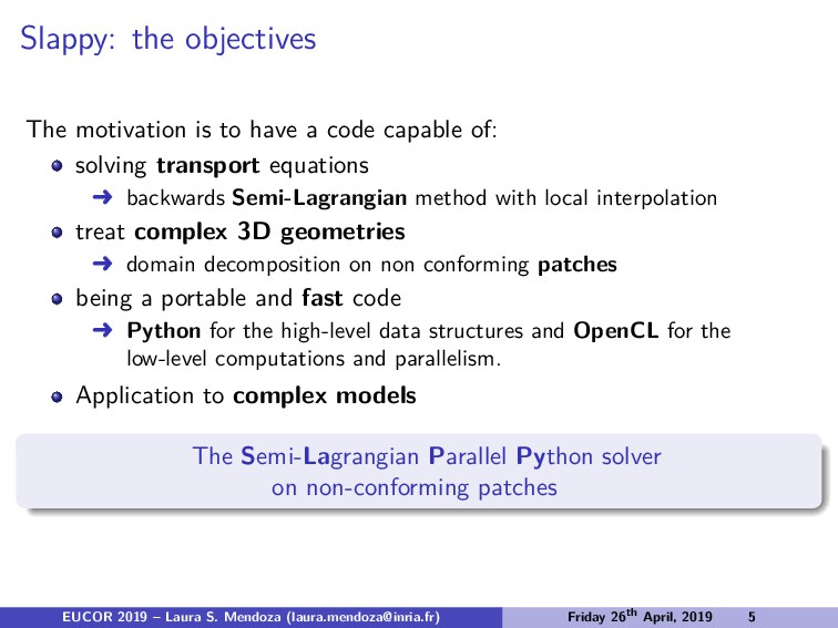
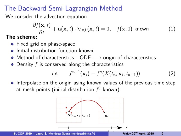
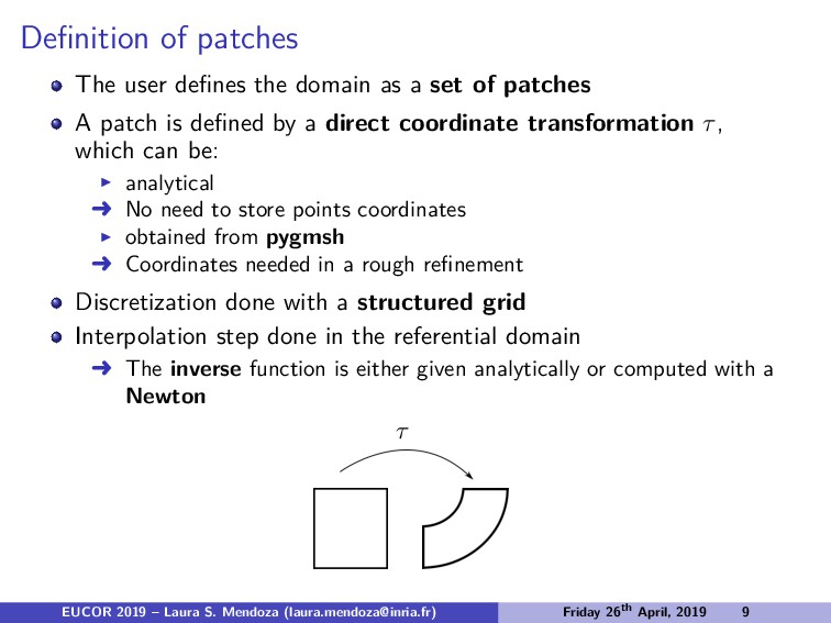
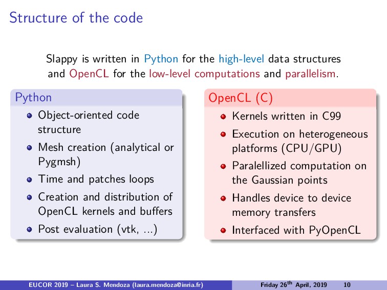
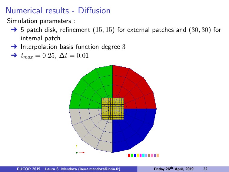
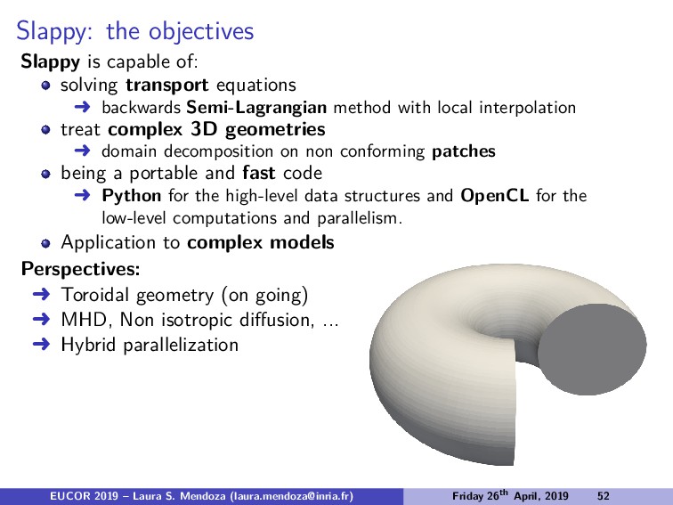
The Python library Slappy was developed to solve transport equations on three-dimensional complex geometries. The geometries are divided into sub-domains called patches. Slappy is based on the backwards Semi-Lagrangian scheme. It uses local continuous Gauss-Lobatto interpolation inside the patches. The interpolation is dis- continuous between patches, thus it handles overlapping and non- conforming patches. The code is written in Python for the high-level data structures and OpenCL for the low-level computations and parallelism.
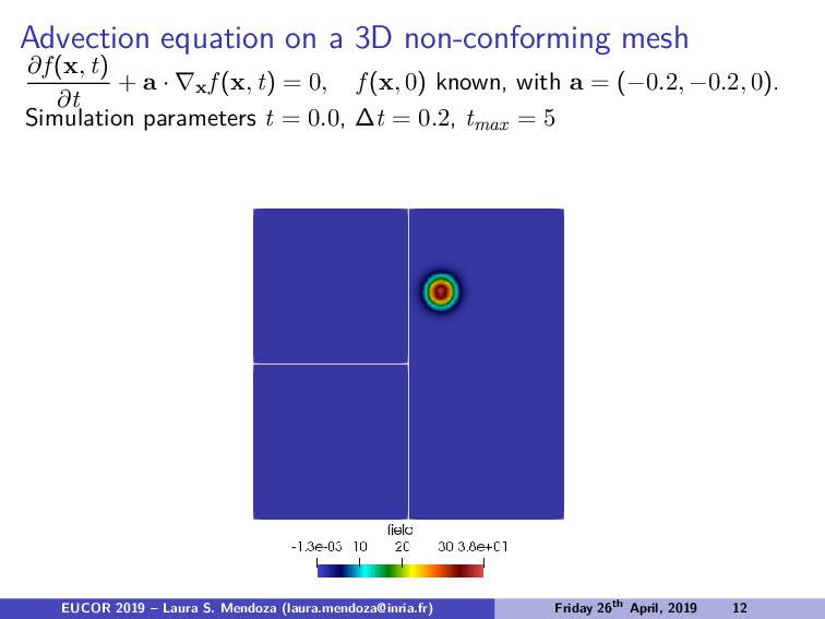
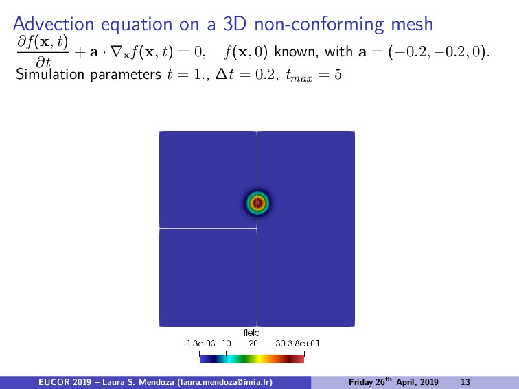
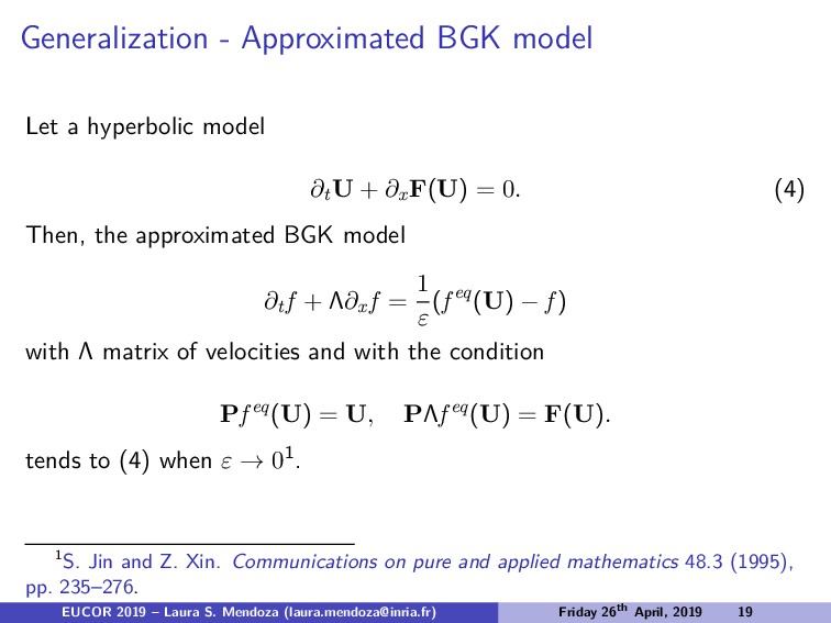
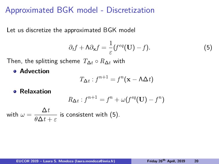
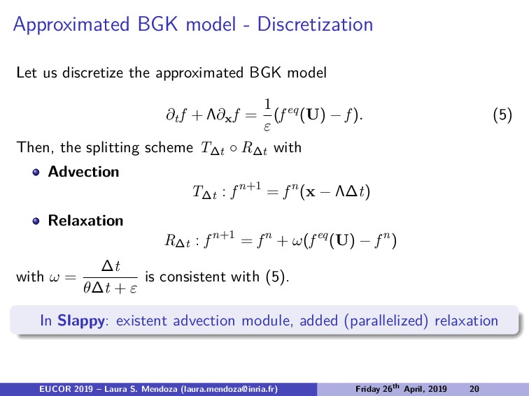
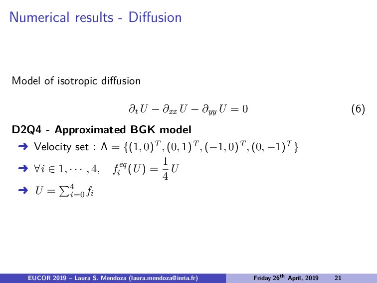
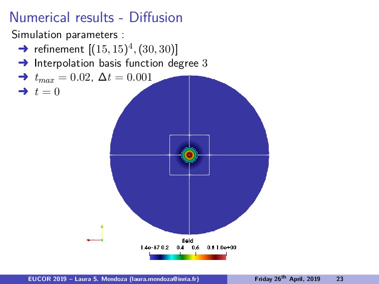
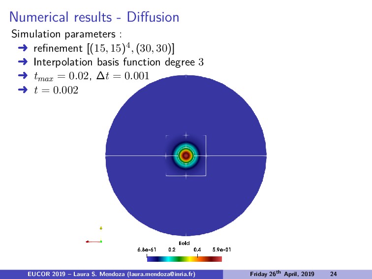
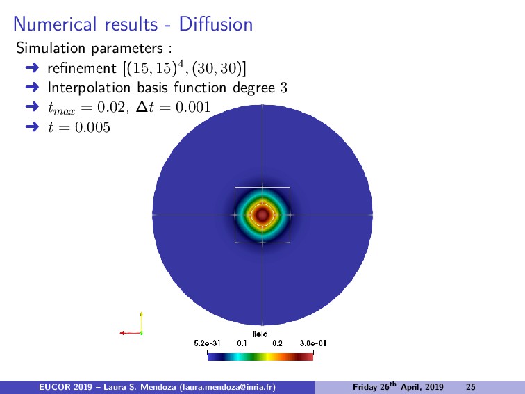
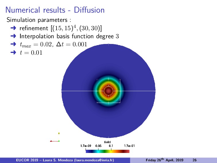
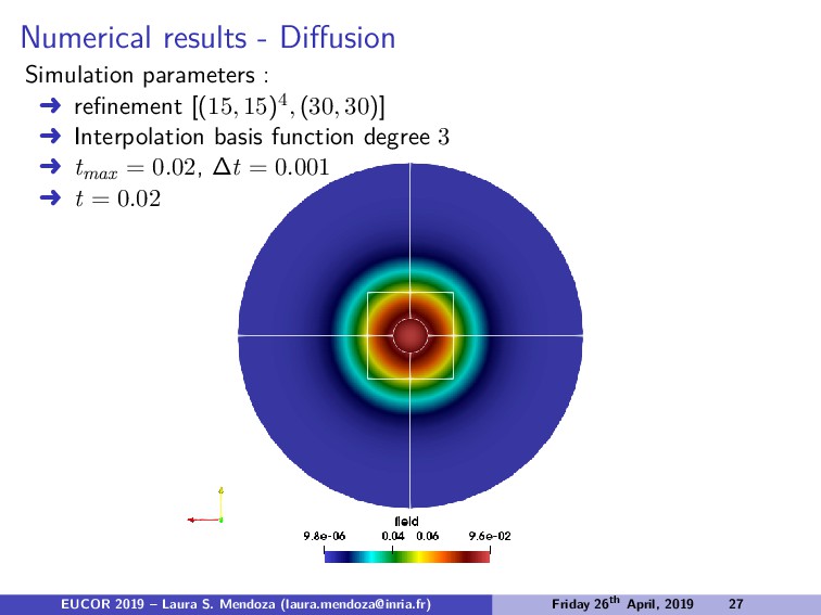
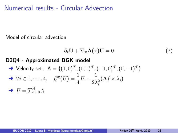
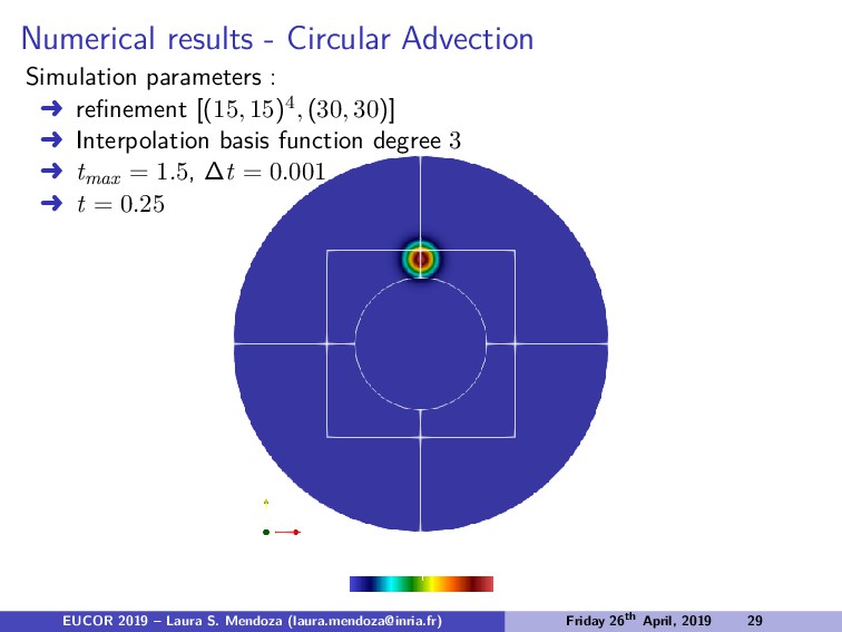
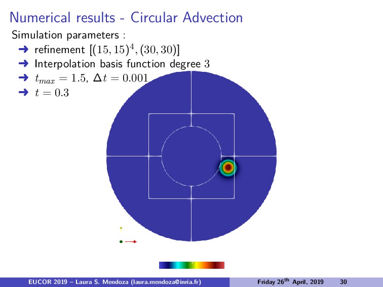
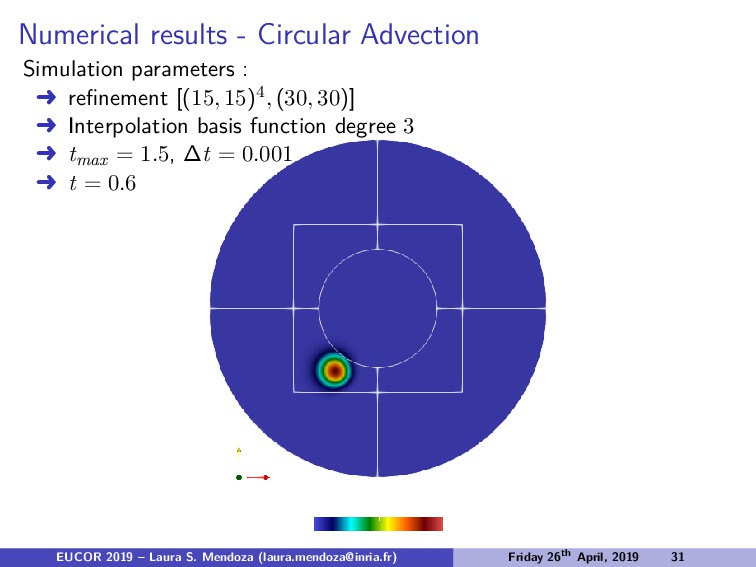
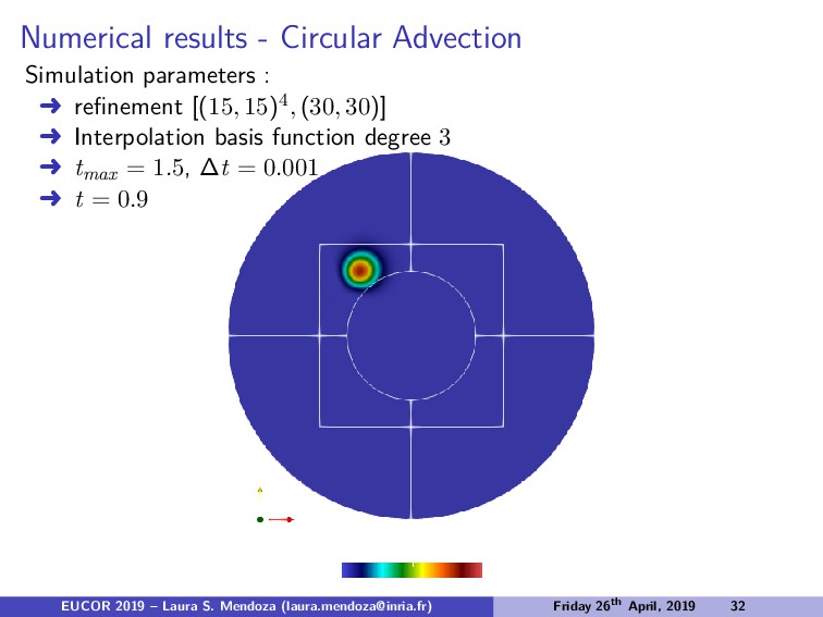
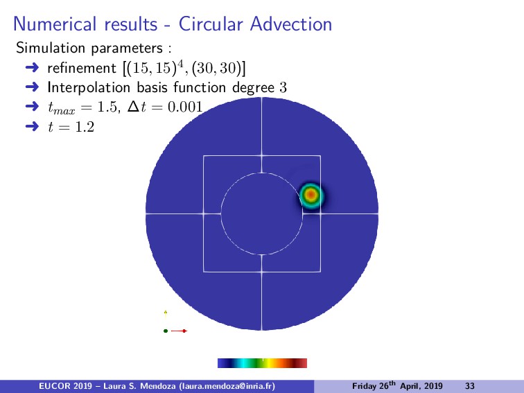
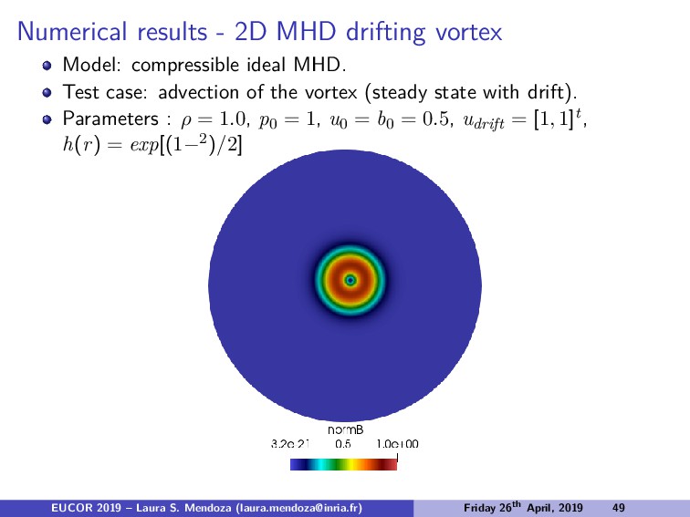
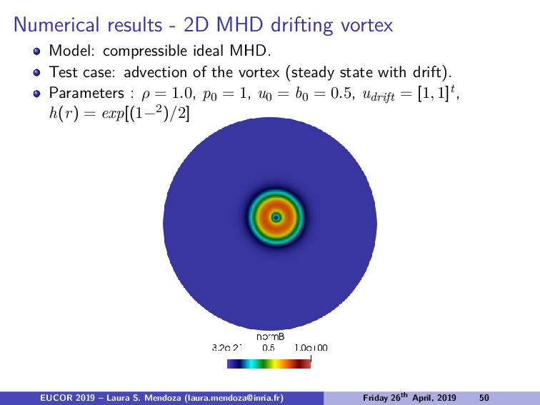
The approximated BGK method allow us to split complex kinetic equations into independent transport equations, solved by the core of the SLaPPy code, and a relaxation step, which was added and parallelized in the code. Thus, we will present the results obtained with the library on linear and circular advections, isotropic diffusion and MHD models, on different geometries formed by non continuous patch.

Transcript

1. Application of the approximated BGK method on a Semi-Lagrangian parallel python solver on non-conforming patches David Coulette Emmanuel Franck1, Philippe Helluy1 Laura S. Mendoza1 1Inria Grand-Est, TONUS TEAM EUCOR 2019, France EUCOR 2019 – Laura S. Mendoza (laura.mendoza@inria.fr) Friday 26th April, 2019 1
2. Context: Energy generation Current solutions present some drawbacks: Limited resources Production of carbon dioxide Radioactive waste Not too efficient Harmful to surrounding environment ⇒ Fusion reactor: cleaner, more reliable, more powerful energy source ? EUCOR 2019 – Laura S. Mendoza (laura.mendoza@inria.fr) Friday 26th April, 2019 2
3. Context: Controlled fusion and magnetic confinement D-T Fusion reaction n n n n n n Deuterium Tritium Helium Temperature > 100 Million◦K. ⇒ Gas composed of positive ions and negative electrons: plasma ⇒ Plasma responds strongly to electromagnetic fields ⇒ Fusion reactor ITER: controlled fusion by magnetic confinment EUCOR 2019 – Laura S. Mendoza (laura.mendoza@inria.fr) Friday 26th April, 2019 3
4. Mathematical context: The Gyrokinetic model Gyrokinetic’s Vlasov equation, 3D-1V, parametric in µ ∂ ∂t + u · ∇x + a ∂ ∂v f (t, x, v , µ) = 0 Fast gyro-motion is averaged out −→ simplified model Self-consistency ensured by a 3D quasi-neutrality equation (solved by 1D FD along the radial direction + Fourier projection) The 5D Gyrokinetic Vlasov equation solved by a time-splitting of Strang −→ 3 advection equations: 1D in the toroidal direction φ; 1D in the parallel velocity v ; 2D in poloidal plane. Advection equations solved using the Semi-Lagrangian scheme Goal: develop a transport and a poisson solver EUCOR 2019 – Laura S. Mendoza (laura.mendoza@inria.fr) Friday 26th April, 2019 4
5. Slappy: the objectives The motivation is to have a code capable of: solving transport equations § backwards Semi-Lagrangian method with local interpolation treat complex 3D geometries § domain decomposition on non conforming patches being a portable and fast code § Python for the high-level data structures and OpenCL for the low-level computations and parallelism. Application to complex models The Semi-Lagrangian Parallel Python solver on non-conforming patches EUCOR 2019 – Laura S. Mendoza (laura.mendoza@inria.fr) Friday 26th April, 2019 5
6. The Backward Semi-Lagrangian Method We consider the advection equation ∂f (x, t) ∂t + a(x, t) · ∇xf (x, t) = 0, f (x, 0) known (1) The scheme: Fixed grid on phase-space Initial distribution function known Method of characteristics : ODE −→ origin of characteristics Density f is conserved along the characteristics i.e. f n+1(xi) = f n(X(tn; xi, tn+1)) (2) Interpolate on the origin using known values of the previous time step at mesh points (initial distribution f 0 known). tn+1 t tn xi X(tn; xi , tn+1) EUCOR 2019 – Laura S. Mendoza (laura.mendoza@inria.fr) Friday 26th April, 2019 6
7. The Backward Semi-Lagrangian Method* We consider the advection equation ∂f (x, t) ∂t + a(x, t) · ∇xf (x, t) = 0, f (x, 0) known (3) The scheme: Fixed grid on space § Mesh refined in Nc cells and each cell L discretized into Nd points (Gauss-Lobatto quadrature) EUCOR 2019 – Laura S. Mendoza (laura.mendoza@inria.fr) Friday 26th April, 2019 7
8. The Backward Semi-Lagrangian Method* We consider the advection equation ∂f (x, t) ∂t + a(x, t) · ∇xf (x, t) = 0, f (x, 0) known (3) The scheme: Fixed grid on space § Mesh refined in Nc cells and each cell L discretized into Nd points (Gauss-Lobatto quadrature) Interpolation step § Local Lagrange interpolation in each cell L using the Lagrange polynomial basis function ϕ of degree d − 1 ˜ f (x, t) = Nd−1 j=0 fL,j (t)ϕL,j (x), x ∈ L EUCOR 2019 – Laura S. Mendoza (laura.mendoza@inria.fr) Friday 26th April, 2019 7
9. The Backward Semi-Lagrangian Method* We consider the advection equation ∂f (x, t) ∂t + a(x, t) · ∇xf (x, t) = 0, f (x, 0) known (3) The scheme: Fixed grid on space § Mesh refined in Nc cells and each cell L discretized into Nd points (Gauss-Lobatto quadrature) Interpolation step § Local Lagrange interpolation in each cell L using the Lagrange polynomial basis function ϕ of degree d − 1 ˜ f (x, t) = Nd−1 j=0 fL,j (t)ϕL,j (x), x ∈ L Advantages: Easy to have high-degree interpolations Possibility to have non conforming and/or overlapping patches Data needed for interpolation close-by memory-wise EUCOR 2019 – Laura S. Mendoza (laura.mendoza@inria.fr) Friday 26th April, 2019 7
10. Multi-patch: the general idea Drawbacks: For ”back-tracing” partciles we need a regular mesh EUCOR 2019 – Laura S. Mendoza (laura.mendoza@inria.fr) Friday 26th April, 2019 8
11. Definition of patches The user defines the domain as a set of patches A patch is defined by a direct coordinate transformation τ, which can be: analytical § No need to store points coordinates obtained from pygmsh § Coordinates needed in a rough refinement Discretization done with a structured grid Interpolation step done in the referential domain § The inverse function is either given analytically or computed with a Newton τ EUCOR 2019 – Laura S. Mendoza (laura.mendoza@inria.fr) Friday 26th April, 2019 9
12. Structure of the code Slappy is written in Python for the high-level data structures and OpenCL for the low-level computations and parallelism. Python Object-oriented code structure Mesh creation (analytical or Pygmsh) Time and patches loops Creation and distribution of OpenCL kernels and buffers Post evaluation (vtk, ...) OpenCL (C) Kernels written in C99 Execution on heterogeneous platforms (CPU/GPU) Paralellized computation on the Gaussian points Handles device to device memory transfers Interfaced with PyOpenCL EUCOR 2019 – Laura S. Mendoza (laura.mendoza@inria.fr) Friday 26th April, 2019 10
13. Advection equation on a 3D non-conforming mesh ∂f (x, t) ∂t + a · ∇xf (x, t) = 0, f (x, 0) known, with a = (−0.2, −0.2, 0). Refinement 20, 15, 20, and degree 3 for each patch. EUCOR 2019 – Laura S. Mendoza (laura.mendoza@inria.fr) Friday 26th April, 2019 11
14. Advection equation on a 3D non-conforming mesh ∂f (x, t) ∂t + a · ∇xf (x, t) = 0, f (x, 0) known, with a = (−0.2, −0.2, 0). Simulation parameters t = 0.0, ∆t = 0.2, tmax = 5 EUCOR 2019 – Laura S. Mendoza (laura.mendoza@inria.fr) Friday 26th April, 2019 12
15. Advection equation on a 3D non-conforming mesh ∂f (x, t) ∂t + a · ∇xf (x, t) = 0, f (x, 0) known, with a = (−0.2, −0.2, 0). Simulation parameters t = 1., ∆t = 0.2, tmax = 5 EUCOR 2019 – Laura S. Mendoza (laura.mendoza@inria.fr) Friday 26th April, 2019 13
16. Advection equation on a 3D non-conforming mesh ∂f (x, t) ∂t + a · ∇xf (x, t) = 0, f (x, 0) known, with a = (−0.2, −0.2, 0). Simulation parameters t = 1.8, ∆t = 0.2, tmax = 5 EUCOR 2019 – Laura S. Mendoza (laura.mendoza@inria.fr) Friday 26th April, 2019 14
17. Advection equation on a 3D non-conforming mesh ∂f (x, t) ∂t + a · ∇xf (x, t) = 0, f (x, 0) known, with a = (−0.2, −0.2, 0). Simulation parameters t = 2.6, ∆t = 0.2, tmax = 5 EUCOR 2019 – Laura S. Mendoza (laura.mendoza@inria.fr) Friday 26th April, 2019 15
18. Advection equation on a 3D non-conforming mesh ∂f (x, t) ∂t + a · ∇xf (x, t) = 0, f (x, 0) known, with a = (−0.2, −0.2, 0). Simulation parameters t = 5, ∆t = 0.2, tmax = 5 EUCOR 2019 – Laura S. Mendoza (laura.mendoza@inria.fr) Friday 26th April, 2019 16
19. Linear Advection - Study of convergence Deg Raf min ||max|| L∞ L2 1 10 4 · 10−7 14.17 2.32 · 10−6 1.43 · 10−5 1 20 4 · 10−12 3.7 3.90 · 10−8 4.49 · 10−7 1 40 8 · 10−17 1.68 3.51 · 10−10 1.01 · 10−8 2 10 −1 · 10−4 1.6 2.46 · 10−6 1.38 · 10−5 2 20 −1 · 10−2 1.08 1.04 · 10−8 1.08 · 10−7 2 40 −2 · 10−4 1.01 1.65 · 10−11 4.82 · 10−10 3 10 −3 · 10−1 1.11 1.81 · 10−7 1.93 · 10−6 3 20 −6 · 10−5 1.005 1.57 · 10−10 4.10 · 10−9 3 40 4 · 10−12 1.006 1.39 · 10−13 8.61 · 10−12 EUCOR 2019 – Laura S. Mendoza (laura.mendoza@inria.fr) Friday 26th April, 2019 17
20. Linear Advection - Scalability Scalability study on CPU: Units Points Time Ite. Exec. Time (s) 1 921 600 25 152 2 921 600 25 71 4 921 600 25 37 8 921 600 25 25 8 1 843 200 25 45 16 1 843 200 25 25 GPU (NVIDIA - CUDA, Tesla K80) vs CPU (64 cores): Device Points Time Ite. Exec. Time (s) GPU 17 203 200 25 75 CPU 17 203 200 25 225 EUCOR 2019 – Laura S. Mendoza (laura.mendoza@inria.fr) Friday 26th April, 2019 18
21. Generalization - Approximated BGK model Let a hyperbolic model ∂tU + ∂xF(U) = 0. (4) Then, the approximated BGK model ∂tf + Λ∂xf = 1 ε (f eq(U) − f ) with Λ matrix of velocities and with the condition Pf eq(U) = U, PΛf eq(U) = F(U). tends to (4) when ε → 01. 1S. Jin and Z. Xin. Communications on pure and applied mathematics 48.3 (1995), pp. 235–276. EUCOR 2019 – Laura S. Mendoza (laura.mendoza@inria.fr) Friday 26th April, 2019 19
22. Approximated BGK model - Discretization Let us discretize the approximated BGK model ∂tf + Λ∂xf = 1 ε (f eq(U) − f ). (5) Then, the splitting scheme T∆t ◦ R∆t with Advection T∆t : f n+1 = f n(x − Λ∆t) Relaxation R∆t : f n+1 = f n + ω(f eq(U) − f n) with ω = ∆t θ∆t + ε is consistent with (5). EUCOR 2019 – Laura S. Mendoza (laura.mendoza@inria.fr) Friday 26th April, 2019 20
23. Approximated BGK model - Discretization Let us discretize the approximated BGK model ∂tf + Λ∂xf = 1 ε (f eq(U) − f ). (5) Then, the splitting scheme T∆t ◦ R∆t with Advection T∆t : f n+1 = f n(x − Λ∆t) Relaxation R∆t : f n+1 = f n + ω(f eq(U) − f n) with ω = ∆t θ∆t + ε is consistent with (5). In Slappy: existent advection module, added (parallelized) relaxation EUCOR 2019 – Laura S. Mendoza (laura.mendoza@inria.fr) Friday 26th April, 2019 20
24. Numerical results - Diffusion Model of isotropic diffusion ∂tU − ∂xxU − ∂yyU = 0 (6) D2Q4 - Approximated BGK model § Velocity set : Λ = {(1, 0)T , (0, 1)T , (−1, 0)T , (0, −1)T } § ∀i ∈ 1, · · · , 4, f eq i (U) = 1 4 U § U = 4 i=0 fi EUCOR 2019 – Laura S. Mendoza (laura.mendoza@inria.fr) Friday 26th April, 2019 21
25. Numerical results - Diffusion Simulation parameters : § 5 patch disk, refinement (15, 15) for external patches and (30, 30) for internal patch § Interpolation basis function degree 3 § tmax = 0.25, ∆t = 0.01 EUCOR 2019 – Laura S. Mendoza (laura.mendoza@inria.fr) Friday 26th April, 2019 22
26. Numerical results - Diffusion Simulation parameters : § refinement [(15, 15)4, (30, 30)] § Interpolation basis function degree 3 § tmax = 0.02, ∆t = 0.001 § t = 0 EUCOR 2019 – Laura S. Mendoza (laura.mendoza@inria.fr) Friday 26th April, 2019 23
27. Numerical results - Diffusion Simulation parameters : § refinement [(15, 15)4, (30, 30)] § Interpolation basis function degree 3 § tmax = 0.02, ∆t = 0.001 § t = 0.002 EUCOR 2019 – Laura S. Mendoza (laura.mendoza@inria.fr) Friday 26th April, 2019 24
28. Numerical results - Diffusion Simulation parameters : § refinement [(15, 15)4, (30, 30)] § Interpolation basis function degree 3 § tmax = 0.02, ∆t = 0.001 § t = 0.005 EUCOR 2019 – Laura S. Mendoza (laura.mendoza@inria.fr) Friday 26th April, 2019 25
29. Numerical results - Diffusion Simulation parameters : § refinement [(15, 15)4, (30, 30)] § Interpolation basis function degree 3 § tmax = 0.02, ∆t = 0.001 § t = 0.01 EUCOR 2019 – Laura S. Mendoza (laura.mendoza@inria.fr) Friday 26th April, 2019 26
30. Numerical results - Diffusion Simulation parameters : § refinement [(15, 15)4, (30, 30)] § Interpolation basis function degree 3 § tmax = 0.02, ∆t = 0.001 § t = 0.02 EUCOR 2019 – Laura S. Mendoza (laura.mendoza@inria.fr) Friday 26th April, 2019 27
31. Numerical results - Circular Advection Model of circular advection ∂tU + ∇xA(x)U = 0 (7) D2Q4 - Approximated BGK model § Velocity set : Λ = {(1, 0)T , (0, 1)T , (−1, 0)T , (0, −1)T } § ∀i ∈ 1, · · · , 4, f eq i (U) = 1 4 U + 1 2λ2 i (Af × λi) § U = 4 i=0 fi EUCOR 2019 – Laura S. Mendoza (laura.mendoza@inria.fr) Friday 26th April, 2019 28
32. Numerical results - Circular Advection Simulation parameters : § refinement [(15, 15)4, (30, 30)] § Interpolation basis function degree 3 § tmax = 1.5, ∆t = 0.001 § t = 0.25 EUCOR 2019 – Laura S. Mendoza (laura.mendoza@inria.fr) Friday 26th April, 2019 29
33. Numerical results - Circular Advection Simulation parameters : § refinement [(15, 15)4, (30, 30)] § Interpolation basis function degree 3 § tmax = 1.5, ∆t = 0.001 § t = 0.3 EUCOR 2019 – Laura S. Mendoza (laura.mendoza@inria.fr) Friday 26th April, 2019 30
34. Numerical results - Circular Advection Simulation parameters : § refinement [(15, 15)4, (30, 30)] § Interpolation basis function degree 3 § tmax = 1.5, ∆t = 0.001 § t = 0.6 EUCOR 2019 – Laura S. Mendoza (laura.mendoza@inria.fr) Friday 26th April, 2019 31
35. Numerical results - Circular Advection Simulation parameters : § refinement [(15, 15)4, (30, 30)] § Interpolation basis function degree 3 § tmax = 1.5, ∆t = 0.001 § t = 0.9 EUCOR 2019 – Laura S. Mendoza (laura.mendoza@inria.fr) Friday 26th April, 2019 32
36. Numerical results - Circular Advection Simulation parameters : § refinement [(15, 15)4, (30, 30)] § Interpolation basis function degree 3 § tmax = 1.5, ∆t = 0.001 § t = 1.2 EUCOR 2019 – Laura S. Mendoza (laura.mendoza@inria.fr) Friday 26th April, 2019 33
37. Numerical results - Circular Advection Simulation parameters : § refinement [(15, 15)4, (30, 30)] § Interpolation basis function degree 3 § tmax = 1.5, ∆t = 0.001 § t = 1.5 EUCOR 2019 – Laura S. Mendoza (laura.mendoza@inria.fr) Friday 26th April, 2019 34
38. Circular Advection - Study of convergence Circular advection on 3P-colella domain, with refinement [raf , raf , 1] for left two patches and [2raf , 2raf , 1] for right patch. The degree is [deg, deg, 1] for all patches. Results after 50 iterations. Deg Raf min ||max|| L∞ L2 3 10 −6.45 · 10−3 1.002 1.78 · 10−5 5.59 · 10−5 3 20 −1.01 · 10−4 0.998 8.76 · 10−7 4.13 · 10−6 3 40 −8.74 · 10−6 0.999 3.31 · 10−8 2.84 · 10−7 GPU (NVIDIA - CUDA, Tesla K80) vs CPU (64 cores): Device Points Time Ite. Exec. Time (s) GPU 2 085 138 50 86 CPU 2 085 138 50 267 EUCOR 2019 – Laura S. Mendoza (laura.mendoza@inria.fr) Friday 26th April, 2019 35
39. Numerical results - Isothermal Euler Model of isothermal Euler ∂tρ + ∇ · (ρu) = 0 ∂tρu + ∇ · (ρu × u + c2ρId) = 0 § Refinement [(15, 15)4, (20, 20)] § Interpolation basis function degree 3 § tmax = 0.5, ∆t = 0.0005 EUCOR 2019 – Laura S. Mendoza (laura.mendoza@inria.fr) Friday 26th April, 2019 36
40. Numerical results - Isothermal Euler § t = 0 EUCOR 2019 – Laura S. Mendoza (laura.mendoza@inria.fr) Friday 26th April, 2019 37
41. Numerical results - Isothermal Euler § t = 0.O625 EUCOR 2019 – Laura S. Mendoza (laura.mendoza@inria.fr) Friday 26th April, 2019 38
42. Numerical results - Isothermal Euler § t = 0.125 EUCOR 2019 – Laura S. Mendoza (laura.mendoza@inria.fr) Friday 26th April, 2019 39
43. Numerical results - Isothermal Euler § t = 0.1875 EUCOR 2019 – Laura S. Mendoza (laura.mendoza@inria.fr) Friday 26th April, 2019 40
44. Numerical results - Isothermal Euler § t = 0.25 EUCOR 2019 – Laura S. Mendoza (laura.mendoza@inria.fr) Friday 26th April, 2019 41
45. Numerical results - Isothermal Euler § t = 0.3125 EUCOR 2019 – Laura S. Mendoza (laura.mendoza@inria.fr) Friday 26th April, 2019 42
46. Numerical results - Isothermal Euler § t = 0.375 EUCOR 2019 – Laura S. Mendoza (laura.mendoza@inria.fr) Friday 26th April, 2019 43
47. Numerical results - Isothermal Euler § t = 0.375 EUCOR 2019 – Laura S. Mendoza (laura.mendoza@inria.fr) Friday 26th April, 2019 44
48. Numerical results - Isothermal Euler § t = 0.4375 EUCOR 2019 – Laura S. Mendoza (laura.mendoza@inria.fr) Friday 26th April, 2019 45
49. Numerical results - Isothermal Euler § t = 0.5 EUCOR 2019 – Laura S. Mendoza (laura.mendoza@inria.fr) Friday 26th April, 2019 46
50. Numerical results - 2D MHD drifting vortex Model: compressible ideal MHD. Test case: advection of the vortex (steady state with drift). Parameters : ρ = 1.0, p0 = 1, u0 = b0 = 0.5, udrift = [1, 1]t, h(r) = exp[(1−2)/2] EUCOR 2019 – Laura S. Mendoza (laura.mendoza@inria.fr) Friday 26th April, 2019 47
51. Numerical results - 2D MHD drifting vortex Model: compressible ideal MHD. Test case: advection of the vortex (steady state with drift). Parameters : ρ = 1.0, p0 = 1, u0 = b0 = 0.5, udrift = [1, 1]t, h(r) = exp[(1 − r2)/2] EUCOR 2019 – Laura S. Mendoza (laura.mendoza@inria.fr) Friday 26th April, 2019 48
52. Numerical results - 2D MHD drifting vortex Model: compressible ideal MHD. Test case: advection of the vortex (steady state with drift). Parameters : ρ = 1.0, p0 = 1, u0 = b0 = 0.5, udrift = [1, 1]t, h(r) = exp[(1−2)/2] EUCOR 2019 – Laura S. Mendoza (laura.mendoza@inria.fr) Friday 26th April, 2019 49
53. Numerical results - 2D MHD drifting vortex Model: compressible ideal MHD. Test case: advection of the vortex (steady state with drift). Parameters : ρ = 1.0, p0 = 1, u0 = b0 = 0.5, udrift = [1, 1]t, h(r) = exp[(1−2)/2] EUCOR 2019 – Laura S. Mendoza (laura.mendoza@inria.fr) Friday 26th April, 2019 50
54. Numerical results - 2D MHD drifting vortex Model: compressible ideal MHD. Test case: advection of the vortex (steady state with drift). Parameters : ρ = 1.0, p0 = 1, u0 = b0 = 0.5, udrift = [1, 1]t, h(r) = exp[(1−2)/2] EUCOR 2019 – Laura S. Mendoza (laura.mendoza@inria.fr) Friday 26th April, 2019 51
55. Slappy: the objectives Slappy is capable of: solving transport equations § backwards Semi-Lagrangian method with local interpolation treat complex 3D geometries § domain decomposition on non conforming patches being a portable and fast code § Python for the high-level data structures and OpenCL for the low-level computations and parallelism. Application to complex models Perspectives: § Toroidal geometry (on going) § MHD, Non isotropic diffusion, ... § Hybrid parallelization EUCOR 2019 – Laura S. Mendoza (laura.mendoza@inria.fr) Friday 26th April, 2019 52