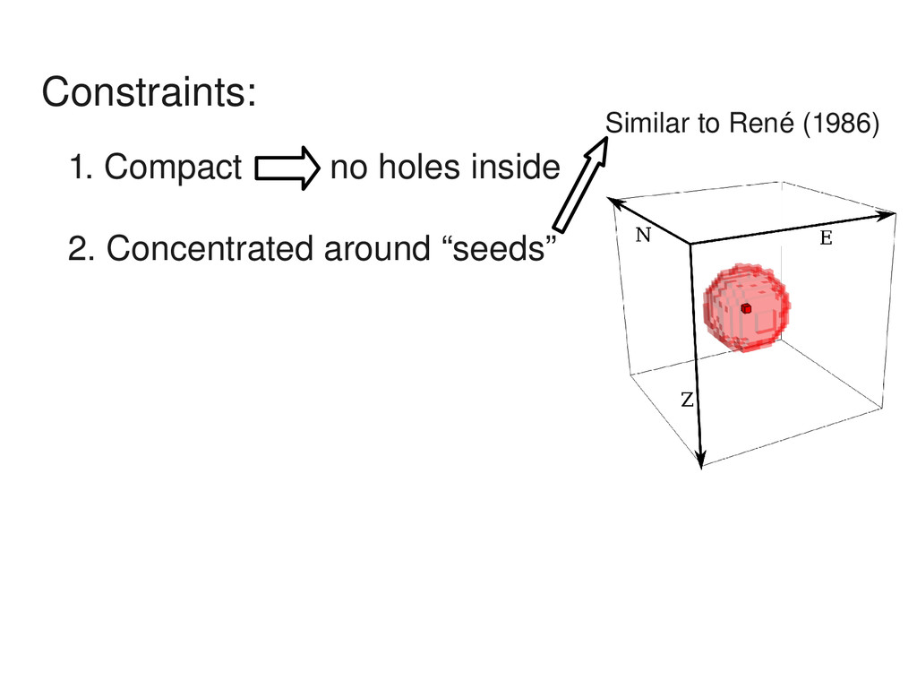
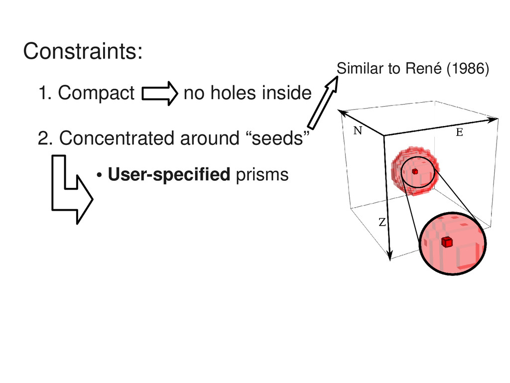
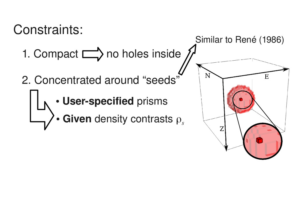
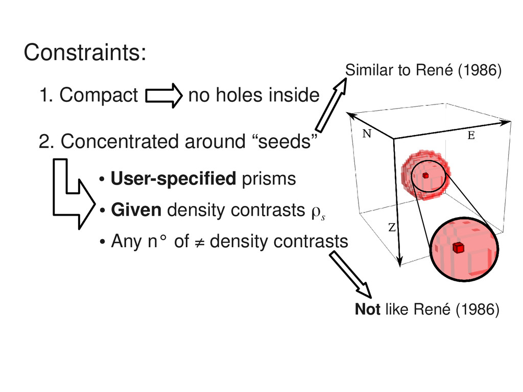
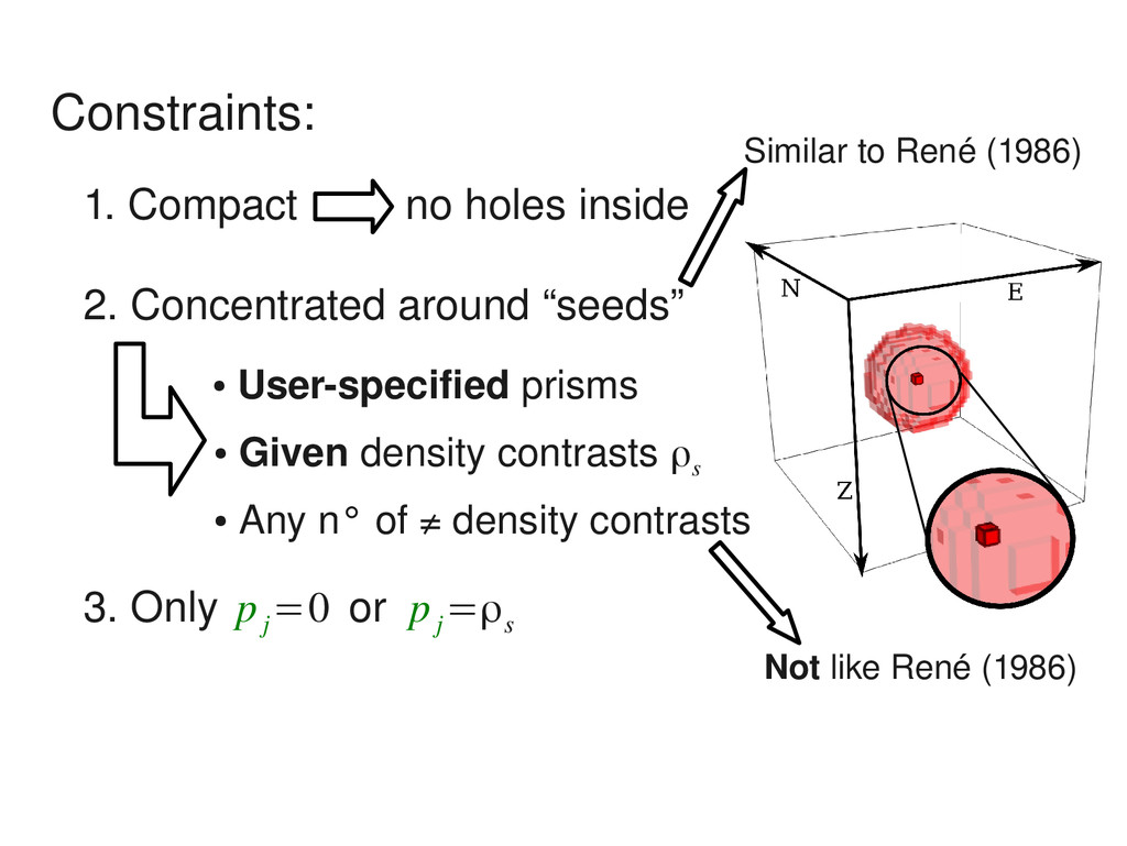
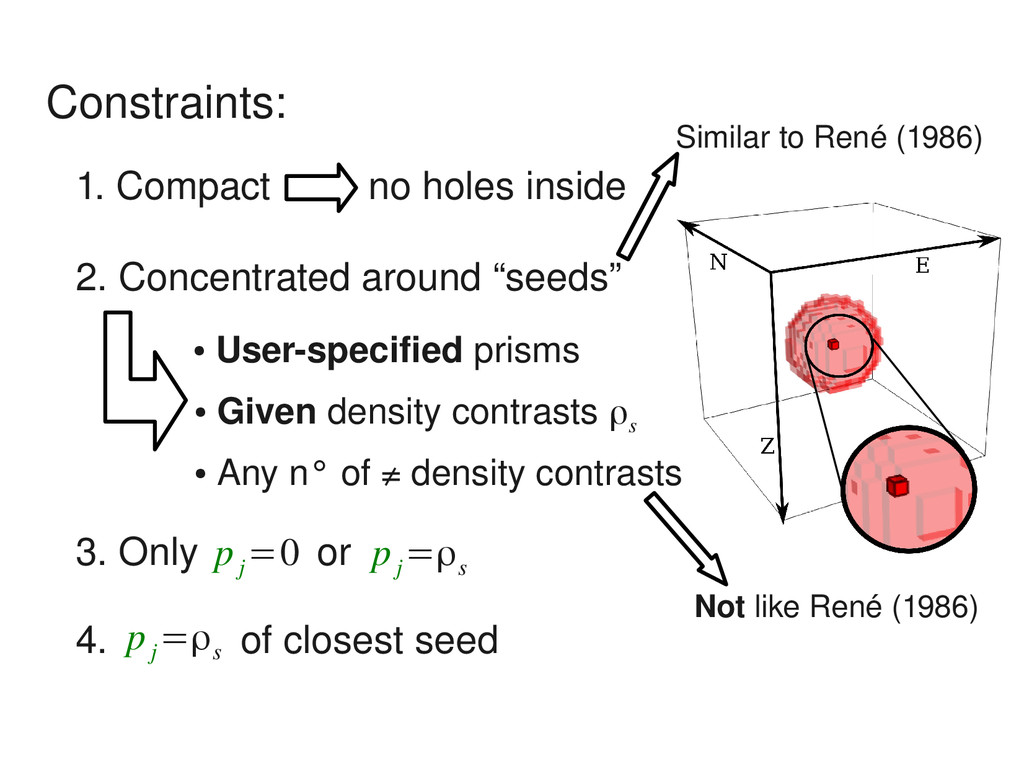
• Userspecified prisms • Given density contrasts 3. Only • Any n° of ≠ density contrasts or p j =0 p j =ρs ρs Similar to René (1986) Not like René (1986)
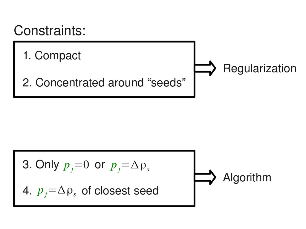
• Userspecified prisms • Given density contrasts 3. Only • Any n° of ≠ density contrasts or p j =0 p j =ρs ρs 4. of closest seed p j =ρs Similar to René (1986) Not like René (1986)
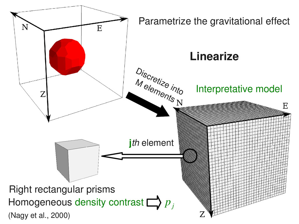
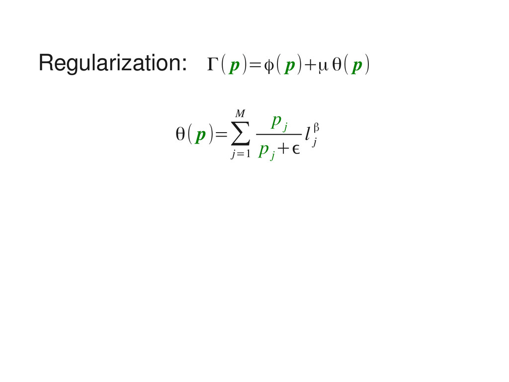
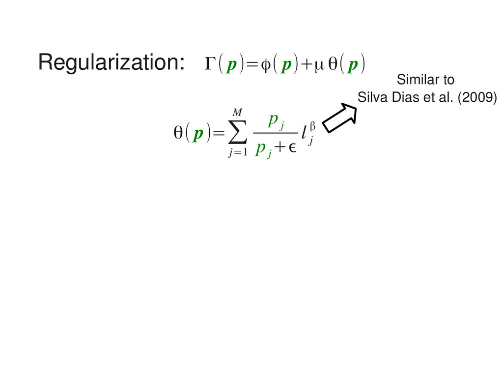
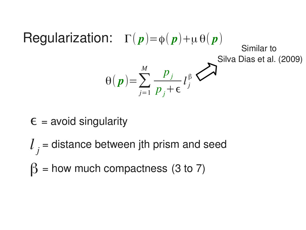
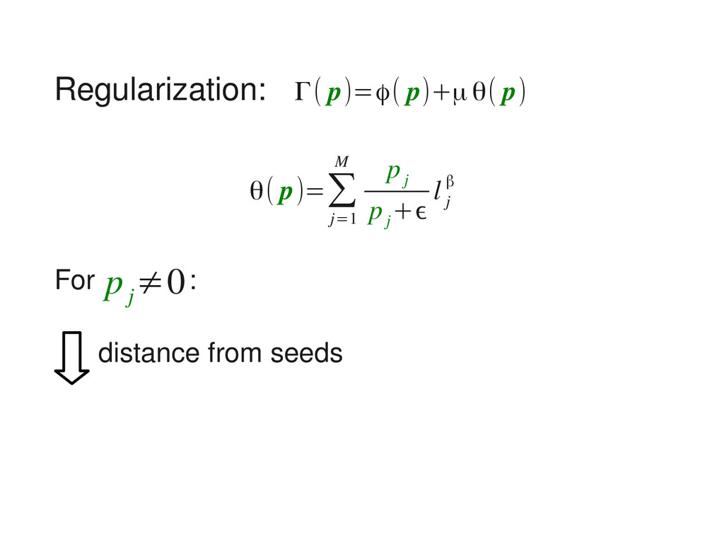
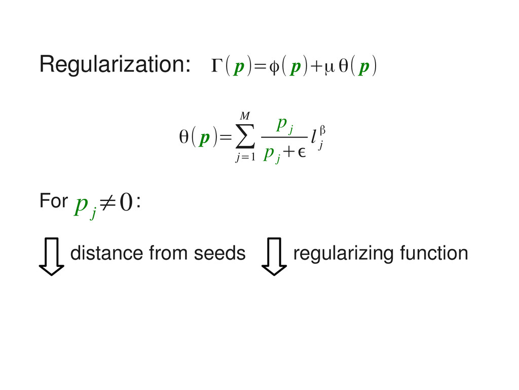
l j β Γ( p)=ϕ( p)+μθ( p) ϵ = avoid singularity l j = distance between jth prism and seed β = how much compactness (3 to 7) Similar to Silva Dias et al. (2009)
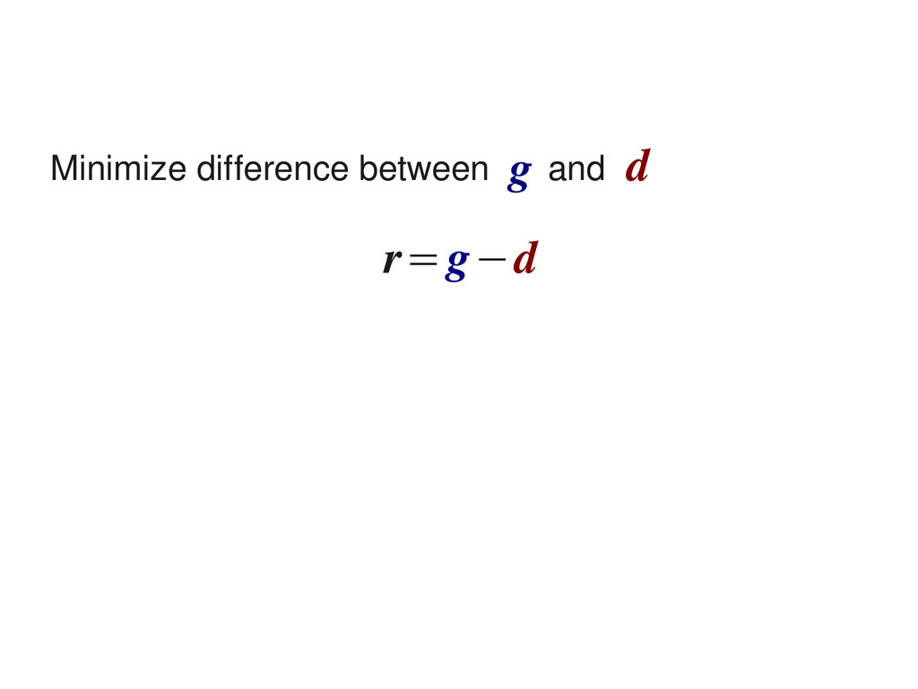
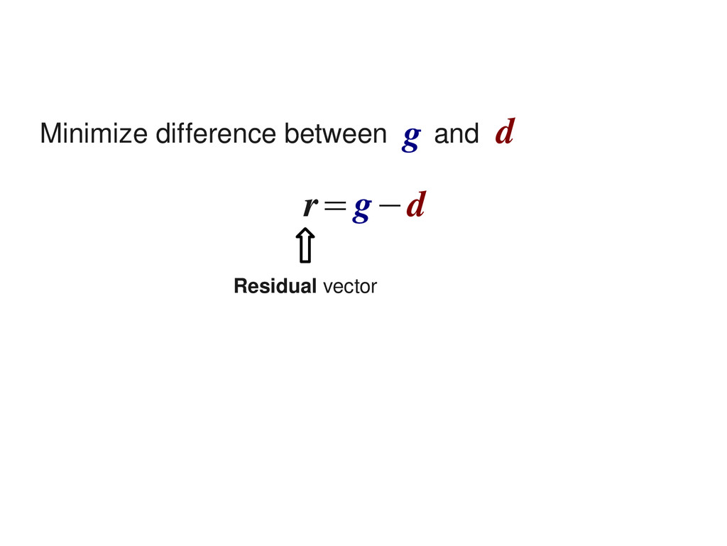
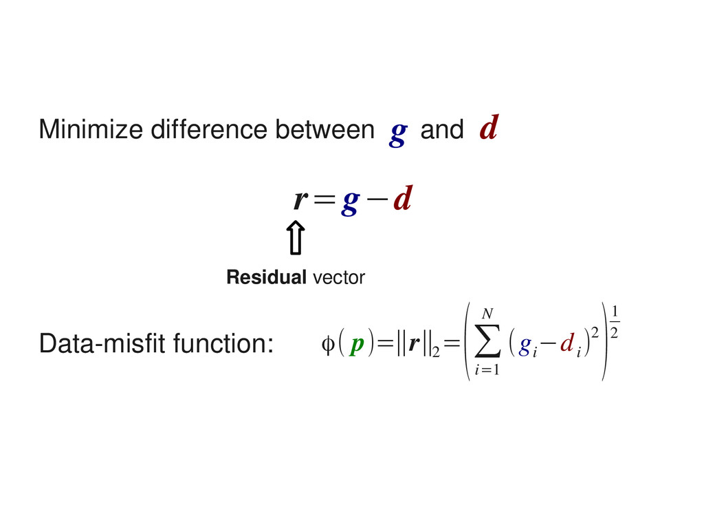
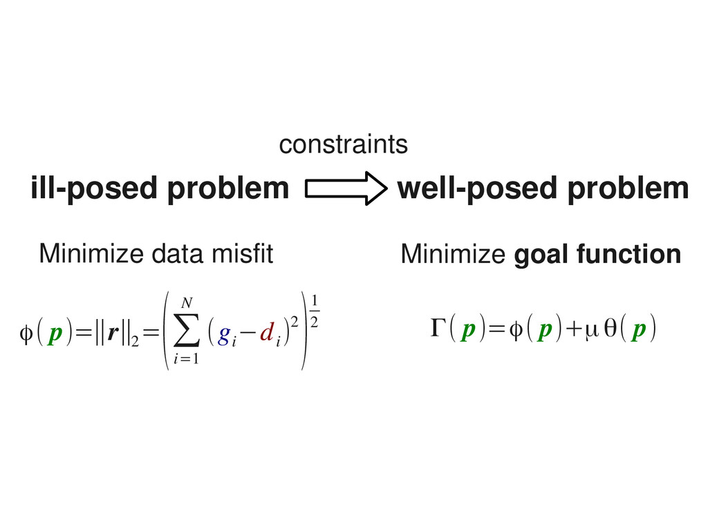
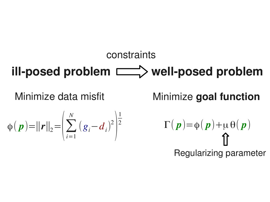
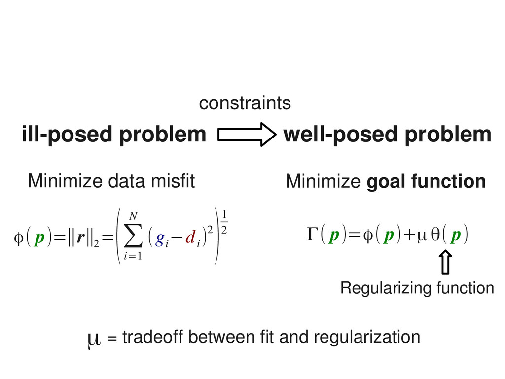
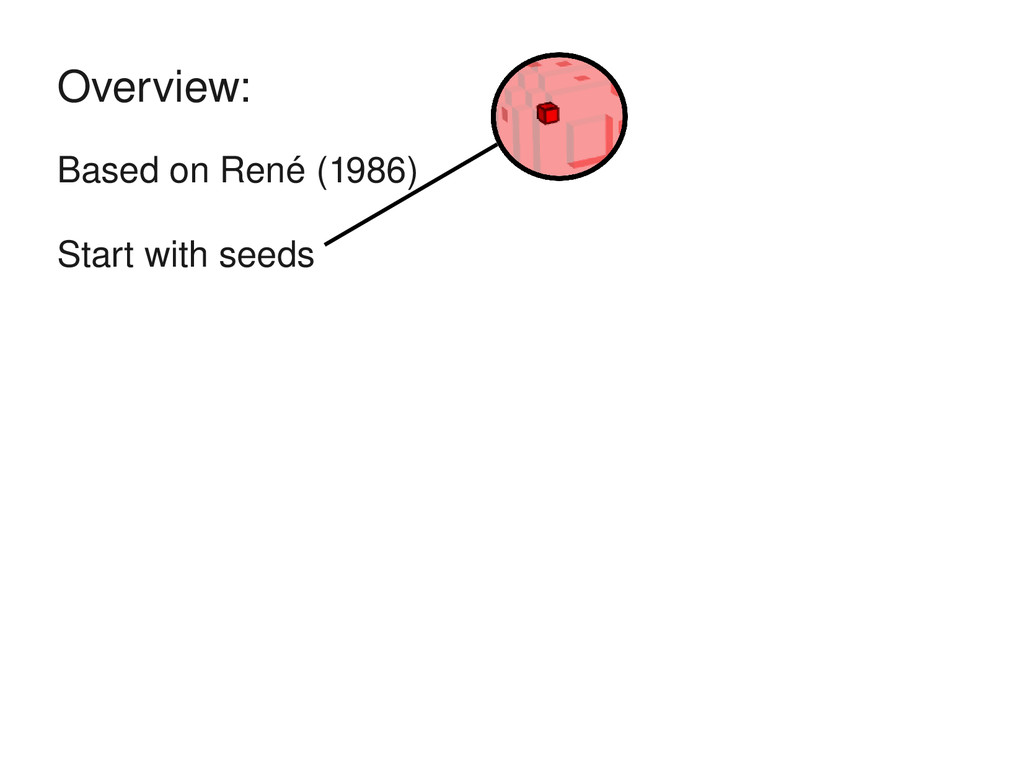
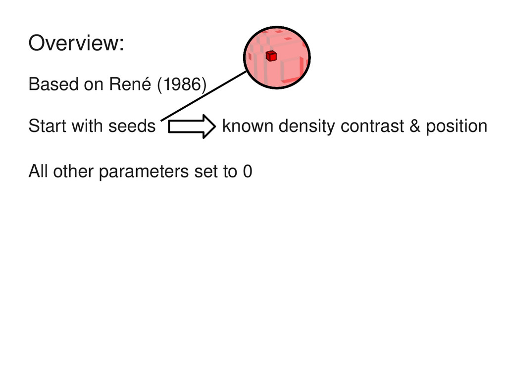
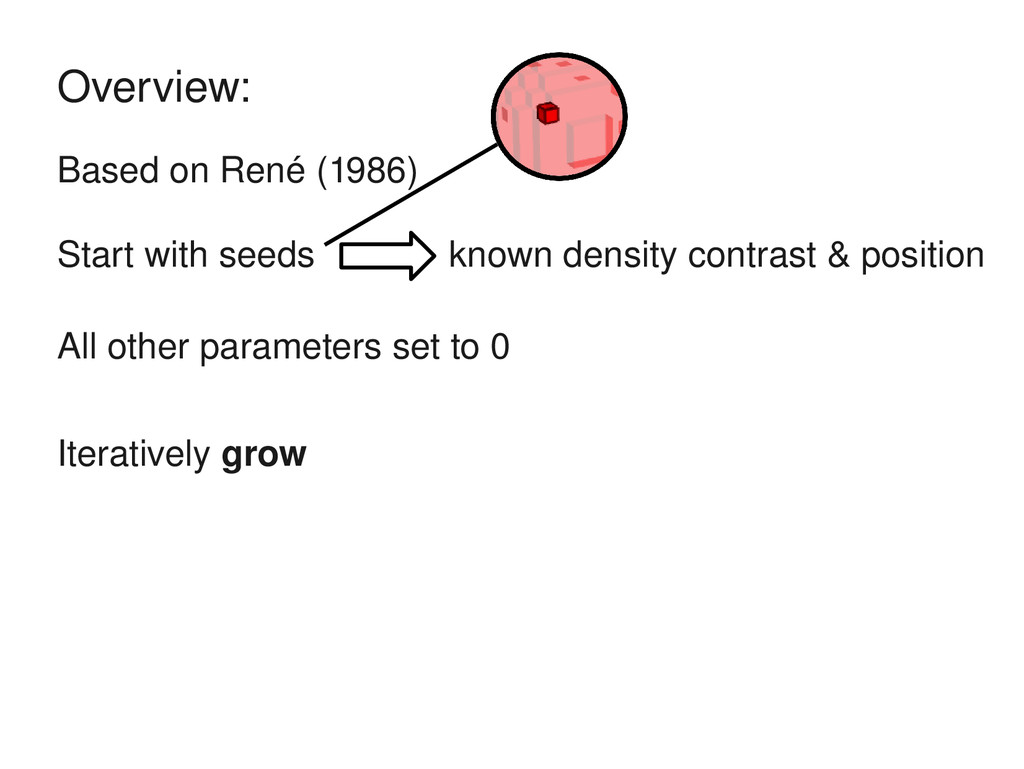
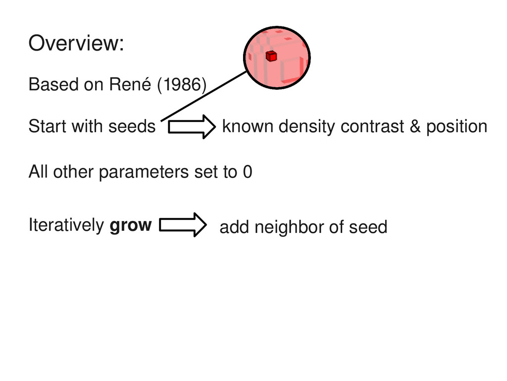
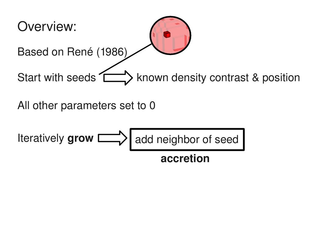
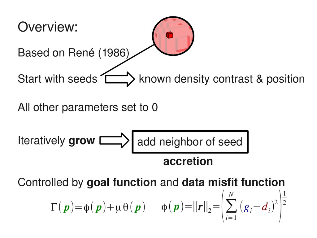
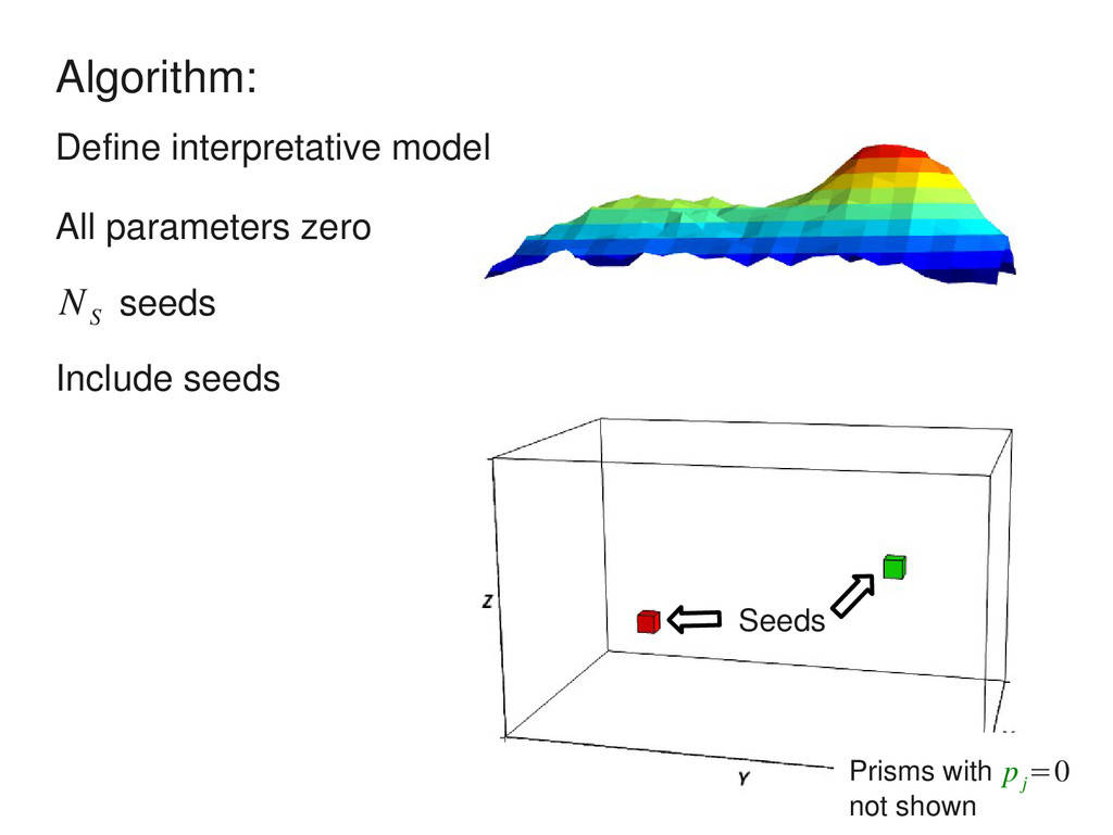
set to 0 Iteratively grow add neighbor of seed accretion Controlled by goal function and data misfit function Overview: Γ( p)=ϕ( p)+μθ( p) ϕ( p)=∥r∥2 = (∑ i=1 N (g i −d i )2 )1 2 known density contrast & position
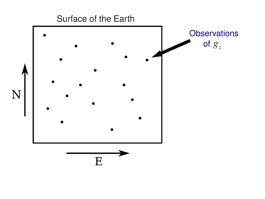
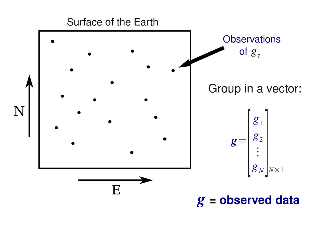
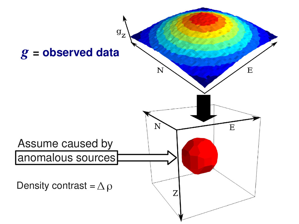
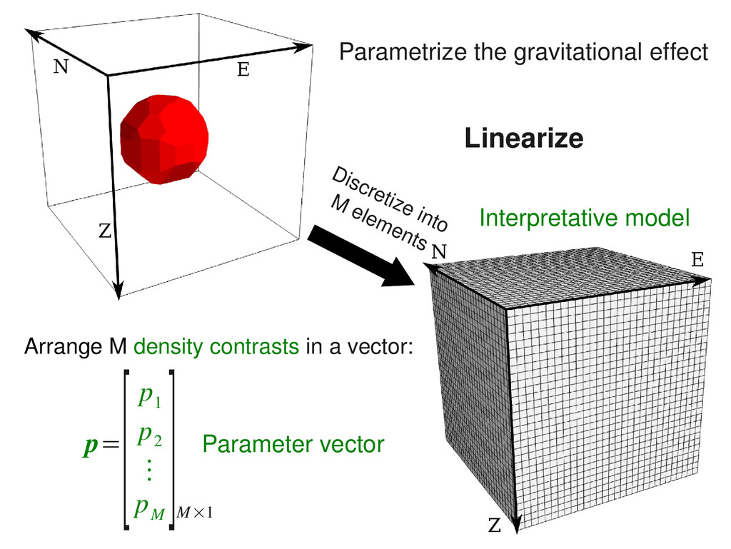
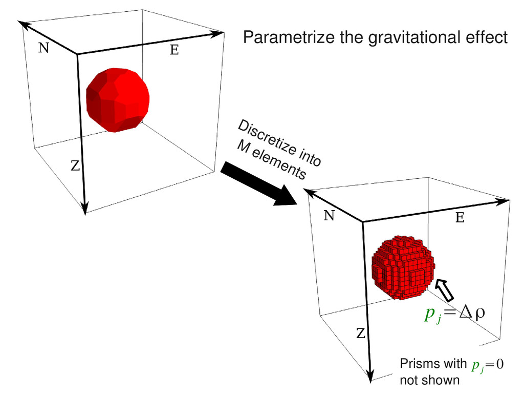
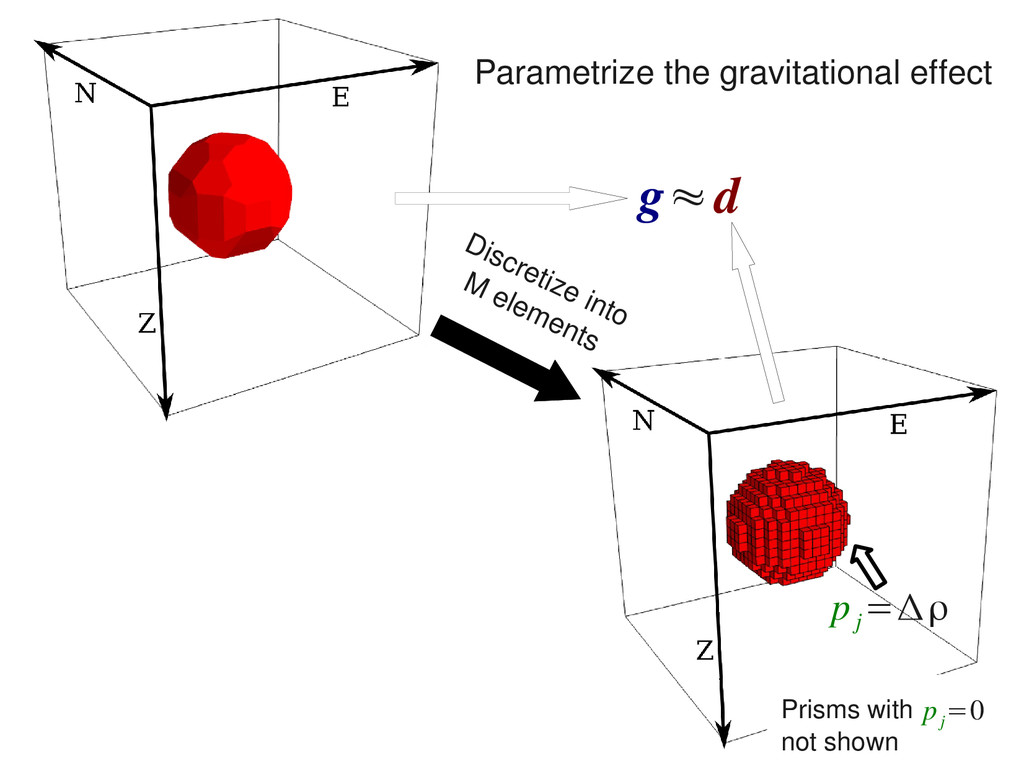
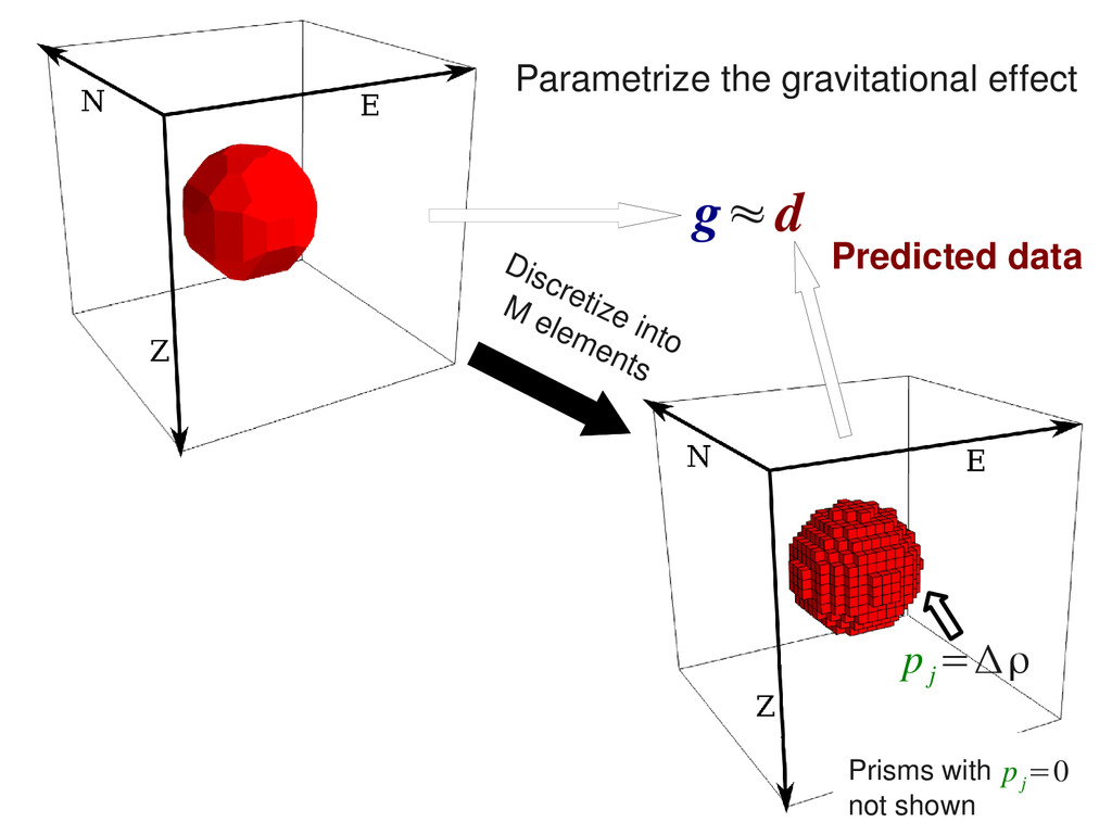
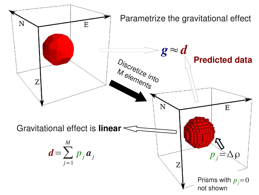
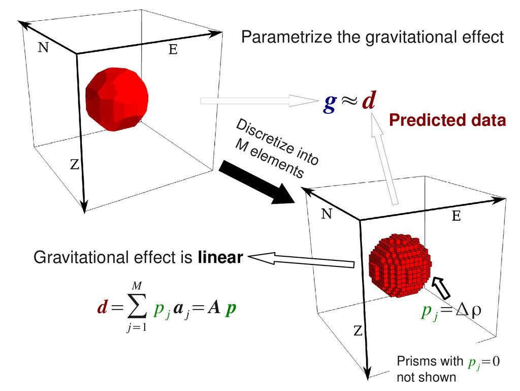
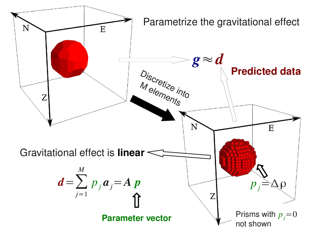
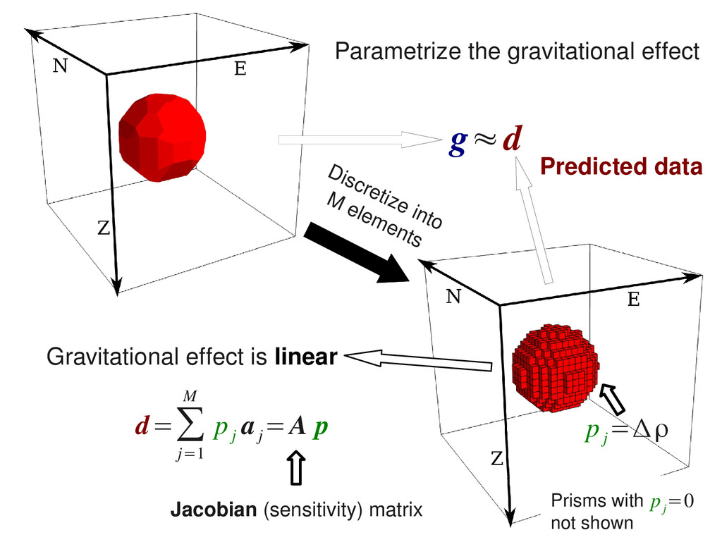
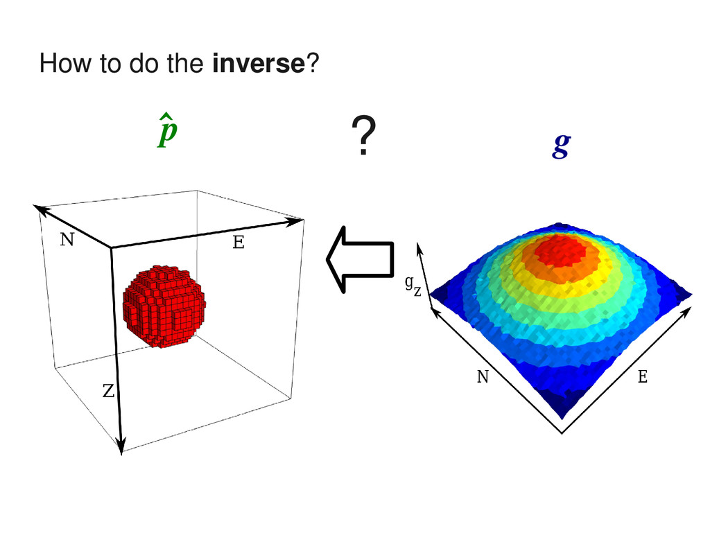
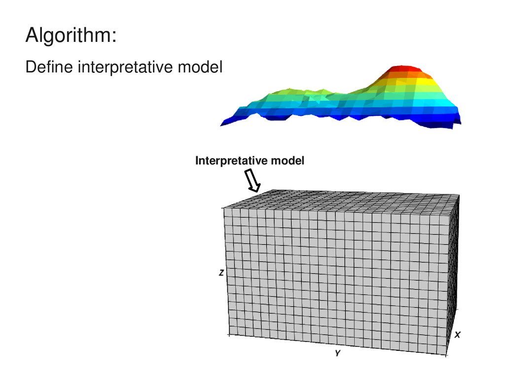
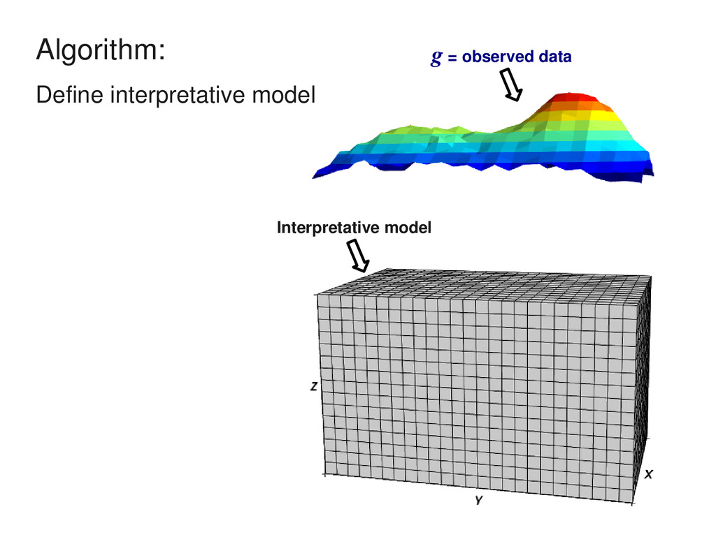
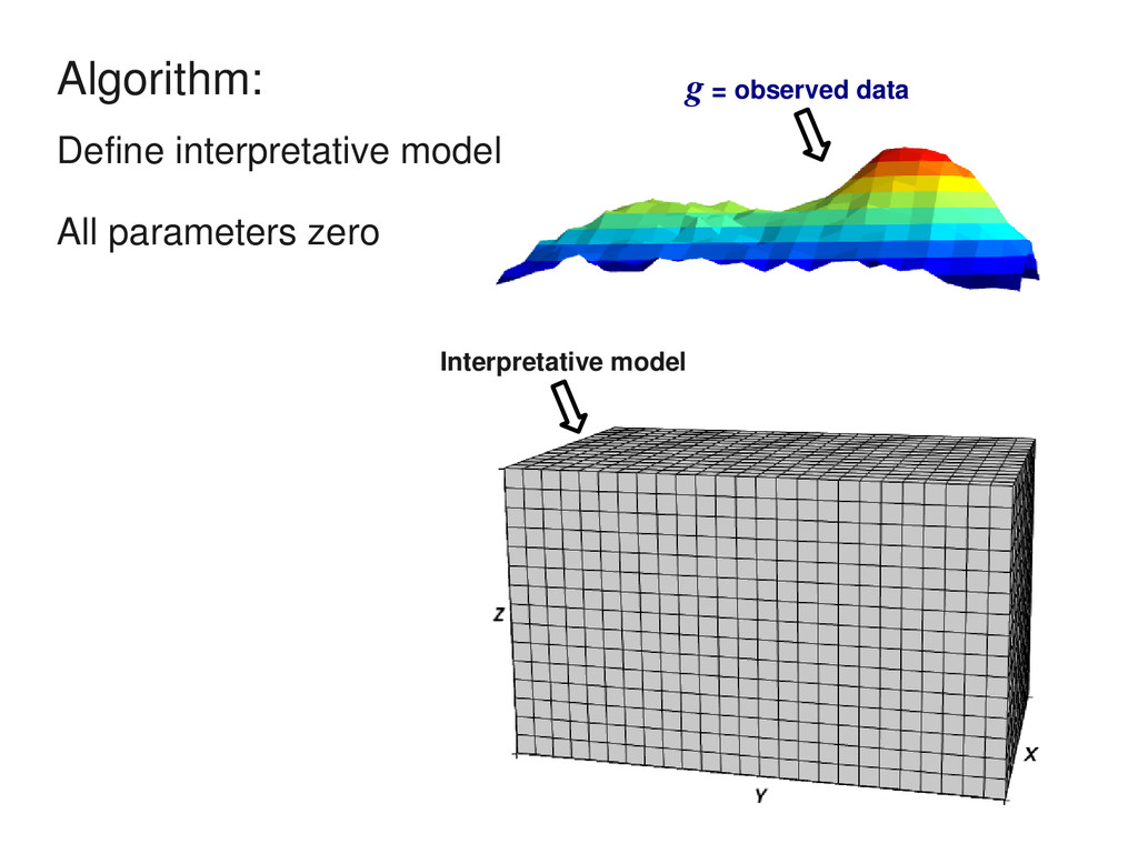
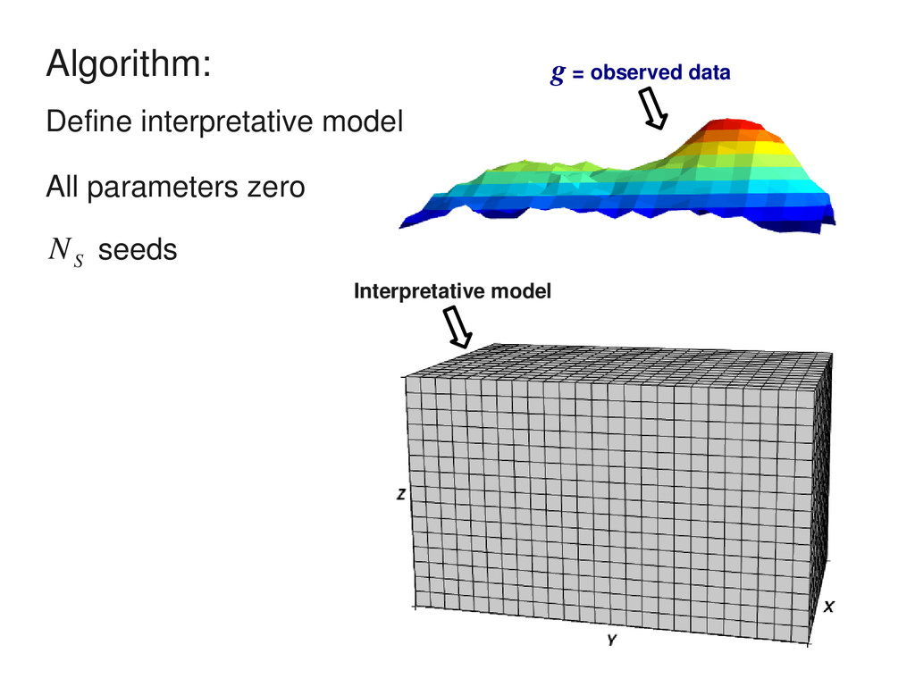
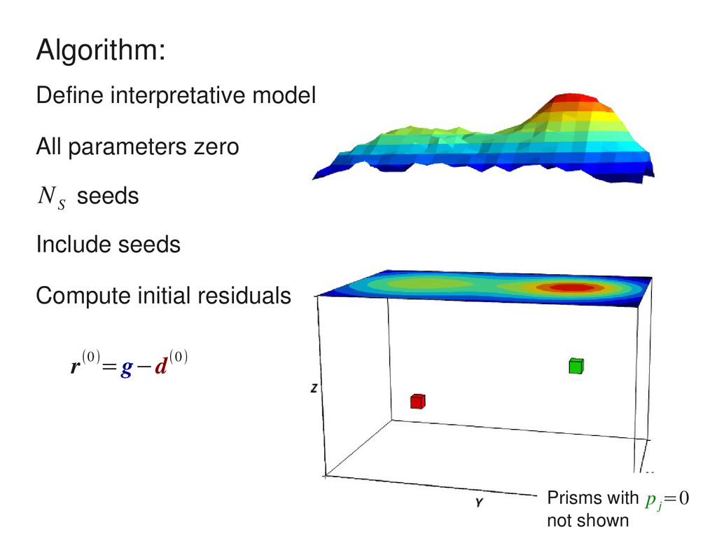
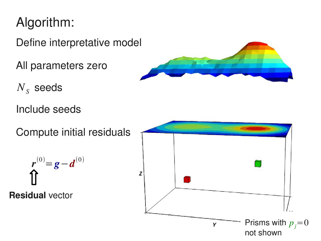
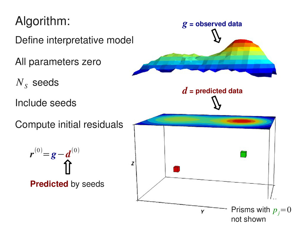
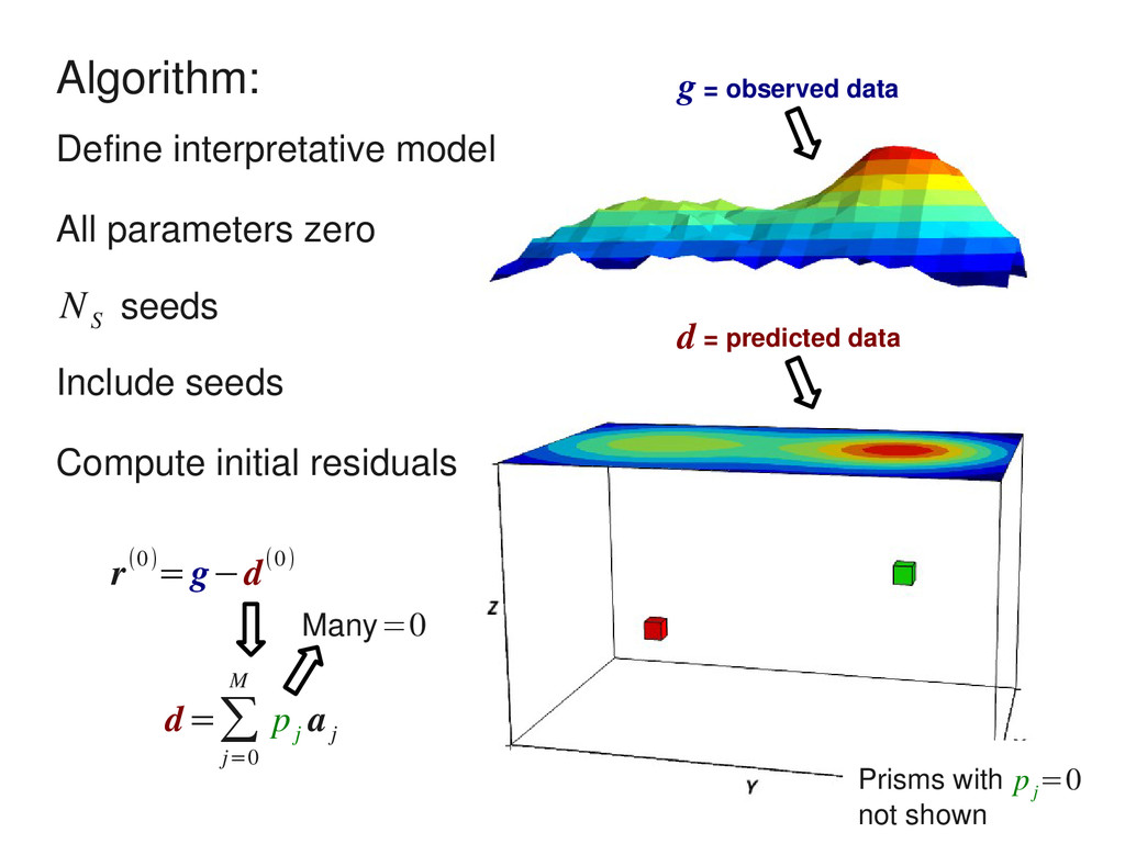
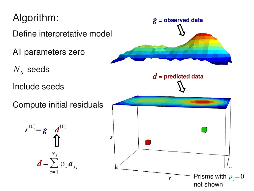
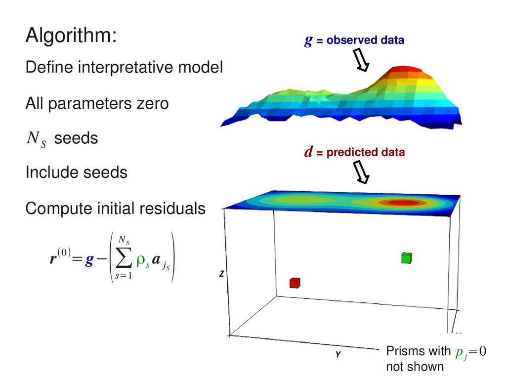
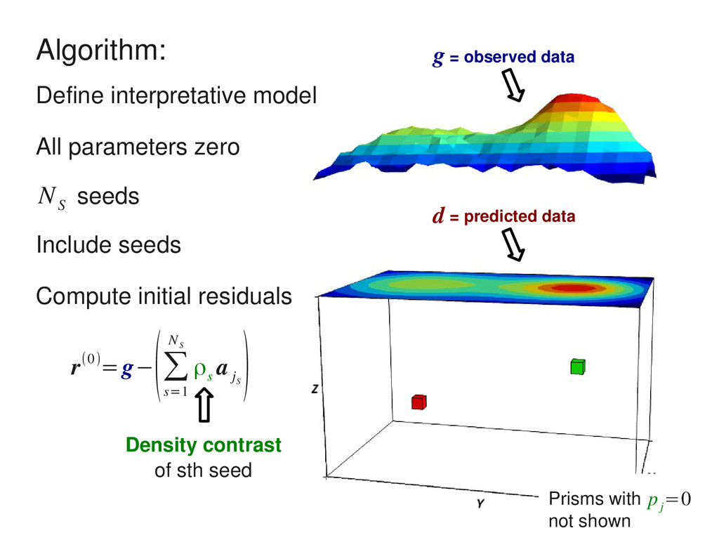
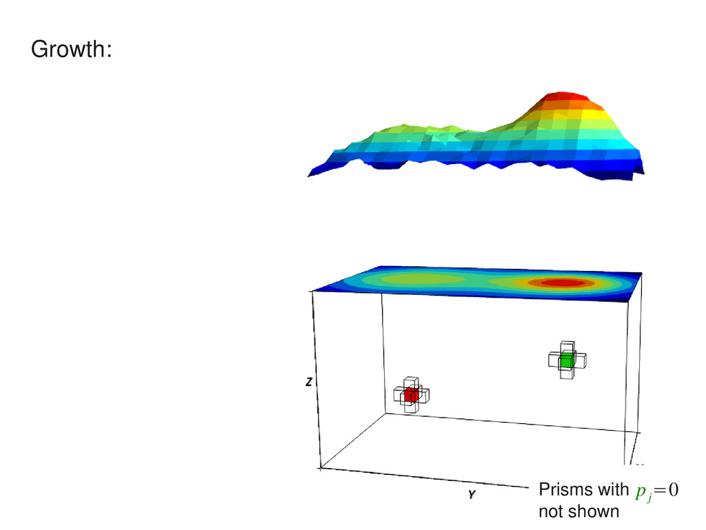
interpretative model All parameters zero Include seeds Compute initial residuals r(0)=g− (∑ s=1 N S ρ s a j S ) Prisms with not shown g = observed data d = predicted data p j =0
Include seeds Compute initial residuals r(0)=g− (∑ s=1 N S ρ s a j S ) Column vector of A Prisms with not shown g = observed data d = predicted data p j =0
Include seeds Compute initial residuals r(0)=g− (∑ s=1 N S ρ s a j S ) Prisms with not shown g = observed data d = predicted data Neighbors Find neighbors of seeds p j =0
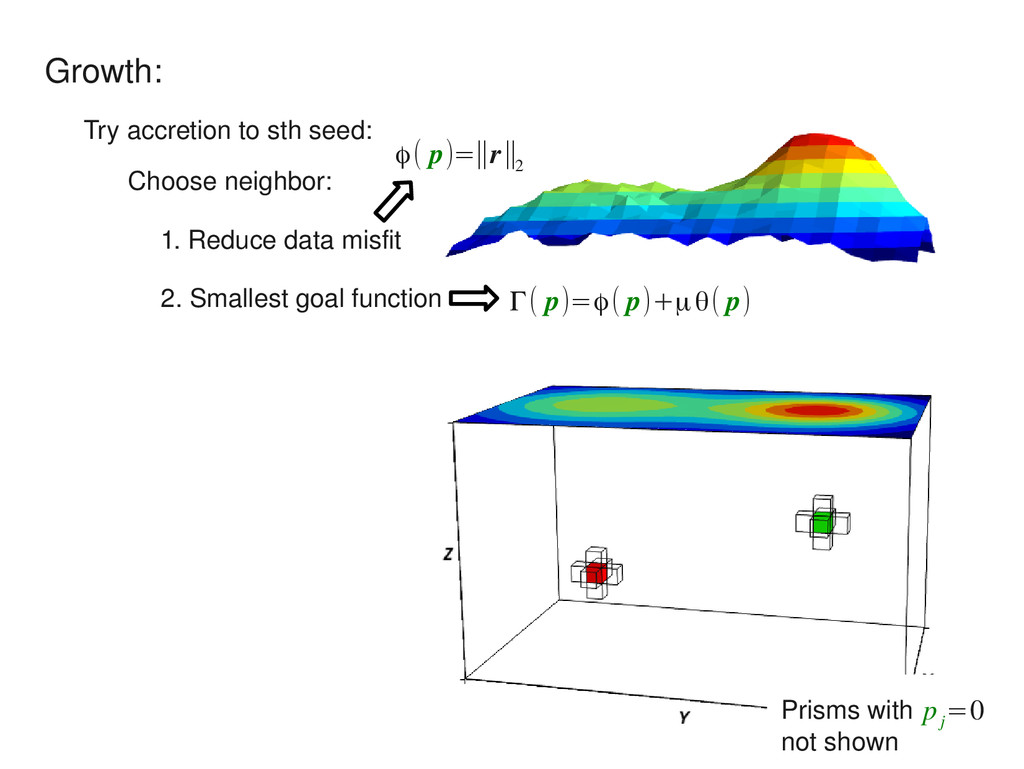
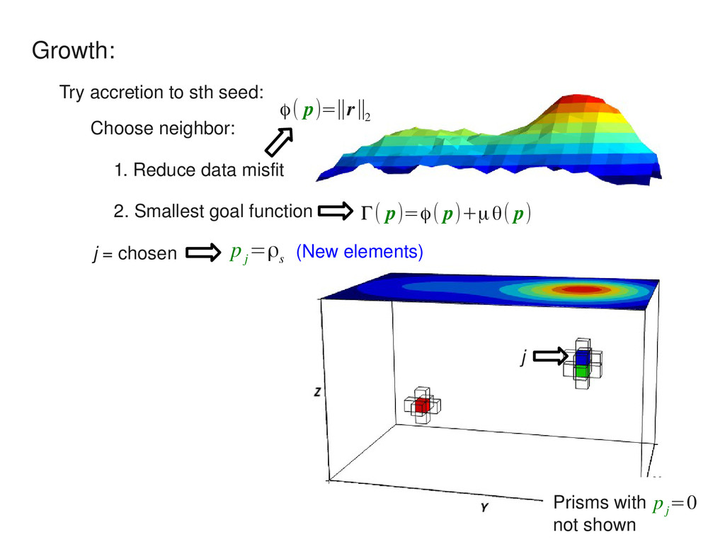
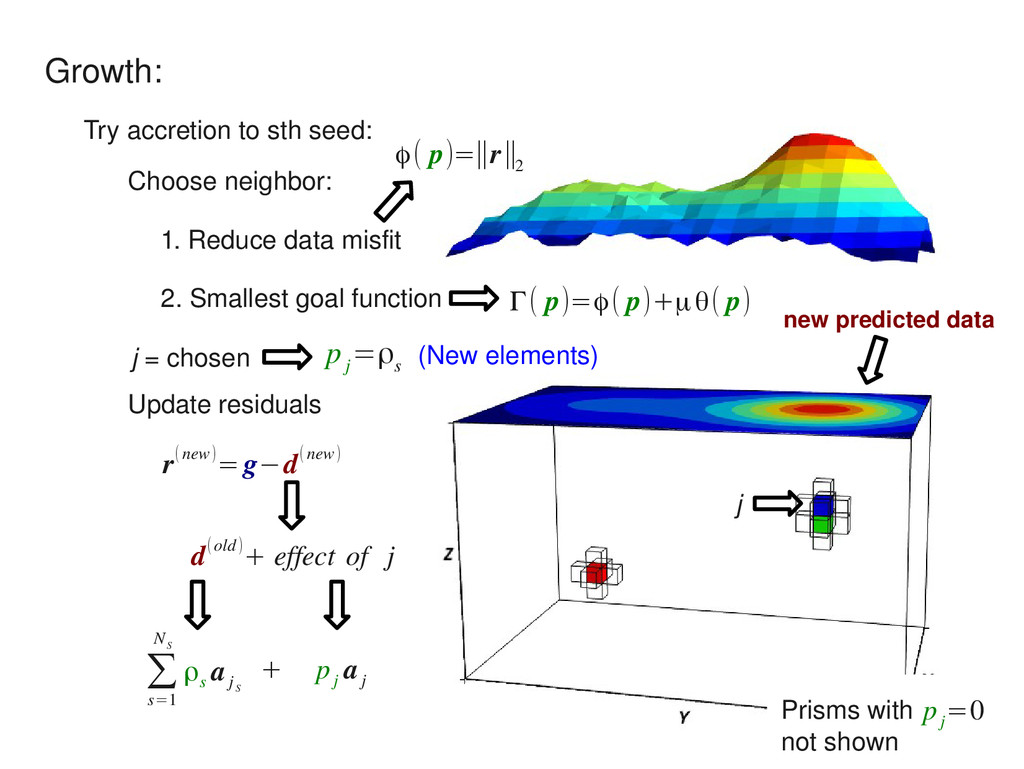
Choose neighbor: 1. Reduce data misfit 2. Smallest goal function ϕ( p)=∥r∥ 2 Γ( p)=ϕ( p)+μθ( p) p j =ρ s j = chosen j p j =0 (New elements) new predicted data
Choose neighbor: 1. Reduce data misfit 2. Smallest goal function ϕ( p)=∥r∥ 2 Γ( p)=ϕ( p)+μθ( p) p j =ρ s j = chosen Update residuals r(new)=g−d(new) p j =0 (New elements) new predicted data j
Choose neighbor: 1. Reduce data misfit 2. Smallest goal function ϕ( p)=∥r∥ 2 Γ( p)=ϕ( p)+μθ( p) p j =ρ s j = chosen Update residuals r(new)=g−d(new) p j =0 (New elements) new predicted data j d(old)+ effect of j
Choose neighbor: 1. Reduce data misfit 2. Smallest goal function ϕ( p)=∥r∥ 2 Γ( p)=ϕ( p)+μθ( p) p j =ρ s j = chosen Update residuals r(new)=g−d(new) p j =0 (New elements) new predicted data j d(old)+ effect of j ∑ s=1 N S ρs a j S p j a j +
Choose neighbor: 1. Reduce data misfit 2. Smallest goal function ϕ( p)=∥r∥ 2 Γ( p)=ϕ( p)+μθ( p) p j =ρ s j = chosen Update residuals r(new)=g−d(new) p j =0 (New elements) new predicted data j d(old)+ effect of j ∑ s=1 N S ρs a j S p j a j +
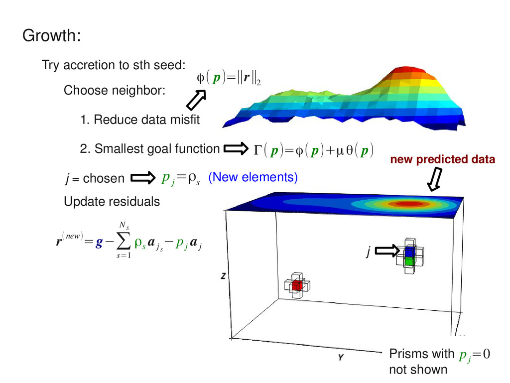
Choose neighbor: 1. Reduce data misfit 2. Smallest goal function ϕ( p)=∥r∥ 2 Γ( p)=ϕ( p)+μθ( p) p j =ρ s j = chosen Update residuals r(new)=g−∑ s=1 N S ρs a j S − p j a j p j =0 (New elements) new predicted data j
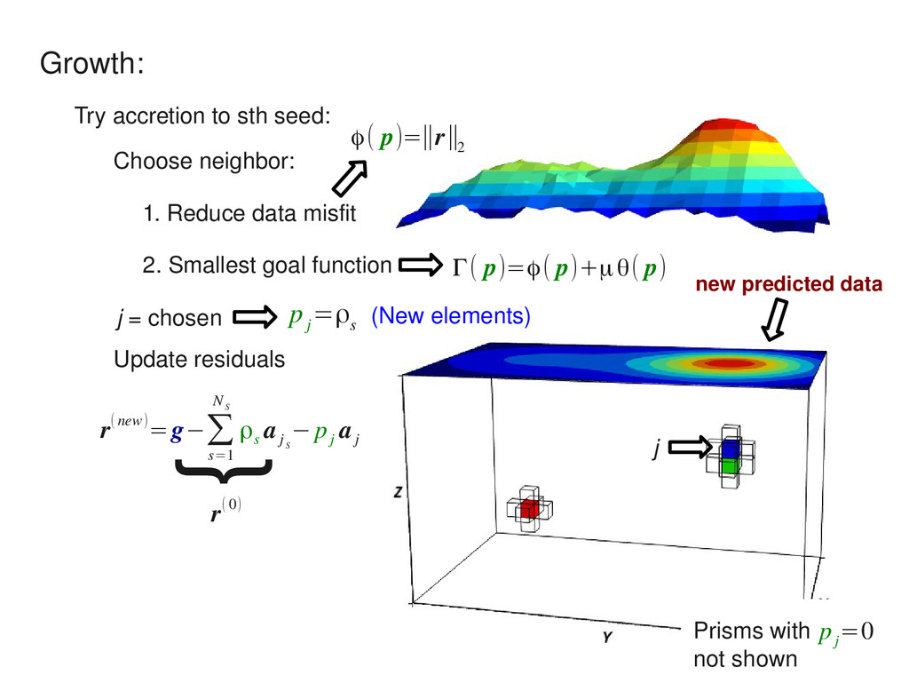
Choose neighbor: 1. Reduce data misfit 2. Smallest goal function ϕ( p)=∥r∥ 2 Γ( p)=ϕ( p)+μθ( p) p j =ρ s j = chosen Update residuals r(new)=g−∑ s=1 N S ρs a j S − p j a j p j =0 (New elements) new predicted data j { r(0)
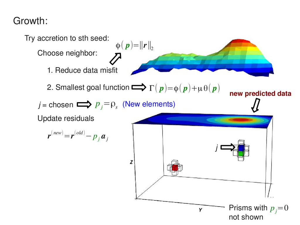
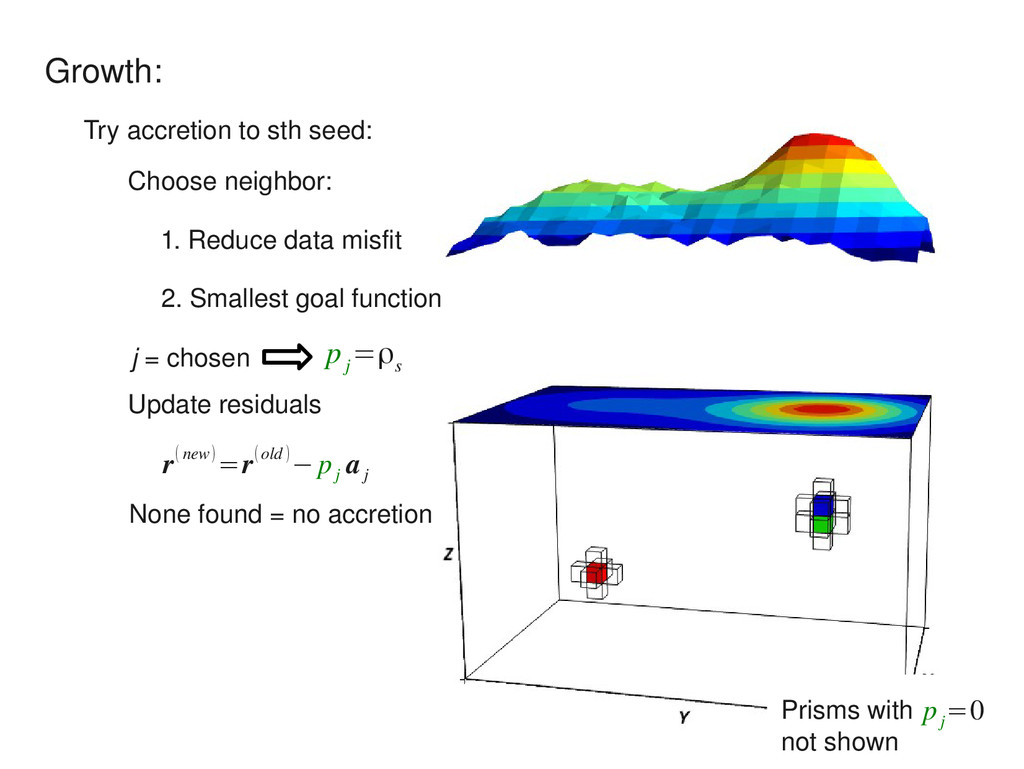
Choose neighbor: 1. Reduce data misfit 2. Smallest goal function ϕ( p)=∥r∥ 2 Γ( p)=ϕ( p)+μθ( p) p j =ρ s j = chosen Update residuals p j =0 (New elements) new predicted data j r(new)=r(old )− p j a j
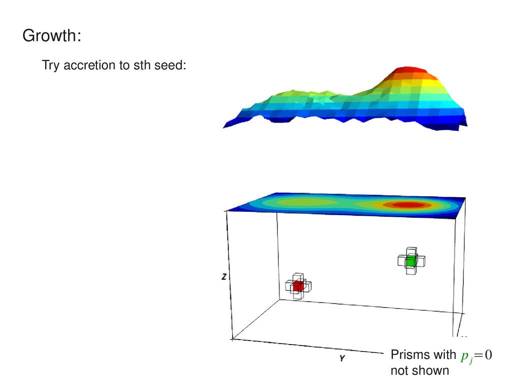
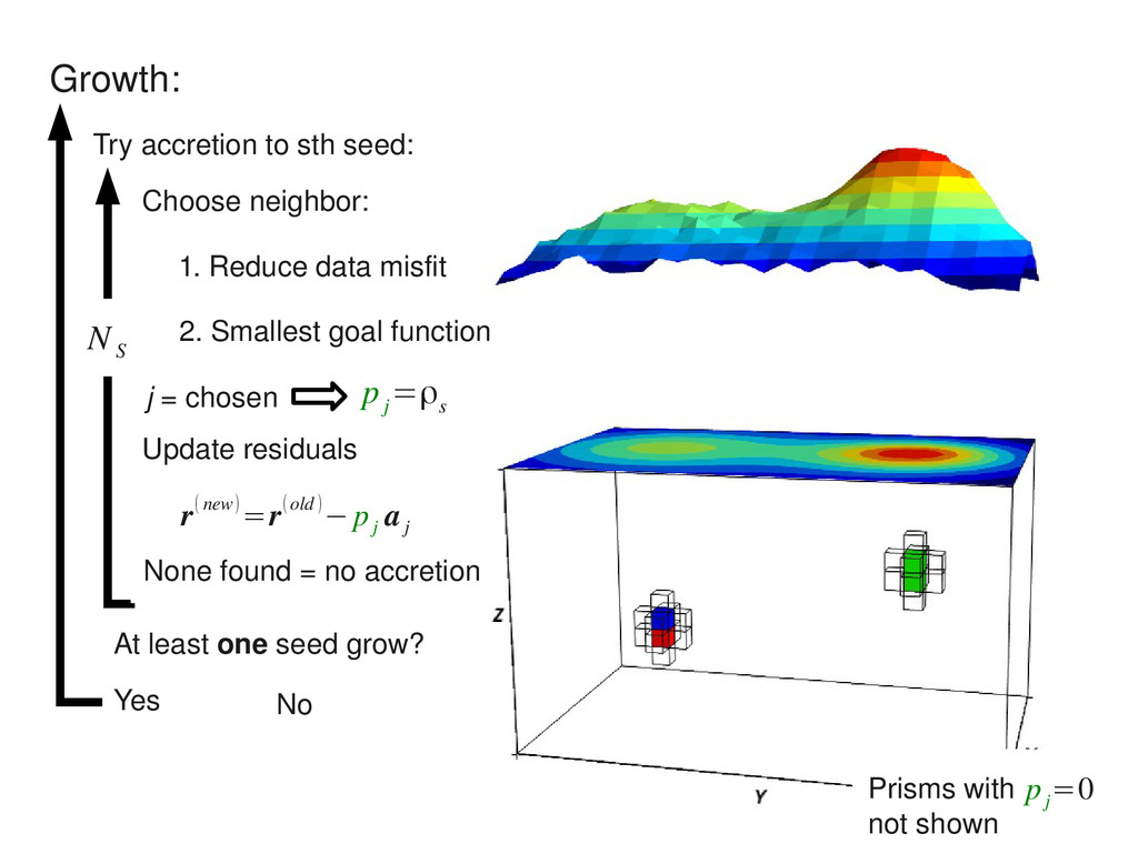
Try accretion to sth seed: 1. Reduce data misfit 2. Smallest goal function p j =ρ s j = chosen Update residuals r(new)=r(old )− p j a j Choose neighbor: p j =0
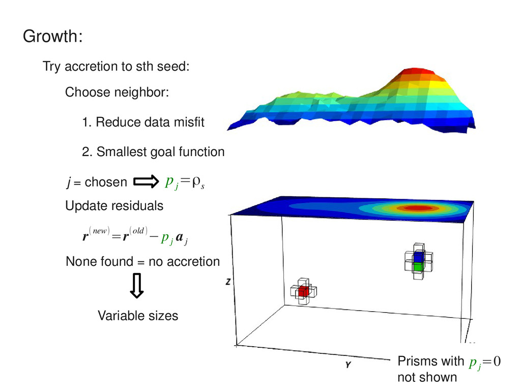
Try accretion to sth seed: 1. Reduce data misfit 2. Smallest goal function p j =ρ s j = chosen Update residuals r(new)=r(old )− p j a j Choose neighbor: Variable sizes p j =0
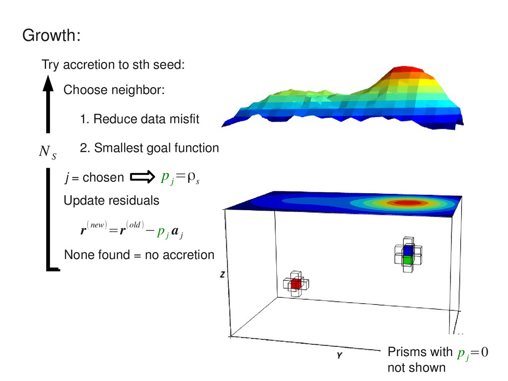
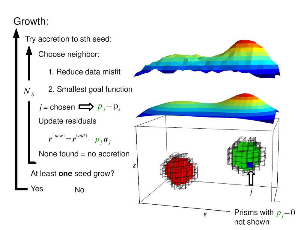
N S Try accretion to sth seed: 1. Reduce data misfit 2. Smallest goal function p j =ρ s j = chosen Update residuals r(new)=r(old )− p j a j Choose neighbor: p j =0
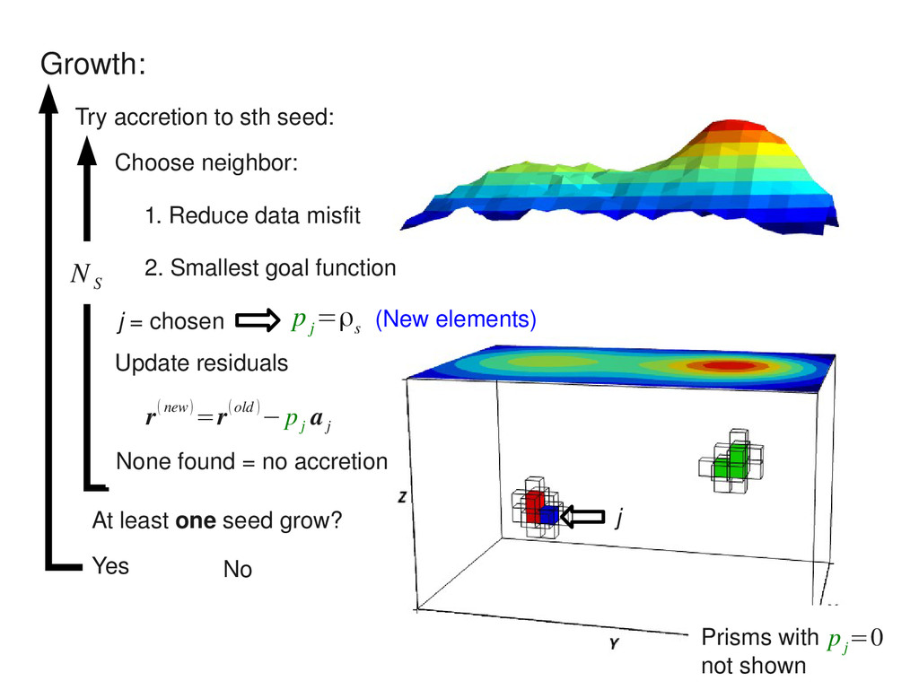
N S Try accretion to sth seed: 1. Reduce data misfit 2. Smallest goal function p j =ρ s j = chosen Update residuals r(new)=r(old )− p j a j Choose neighbor: p j =0 (New elements) j
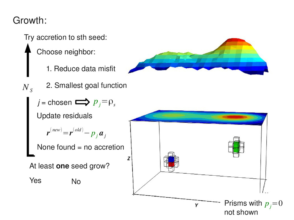
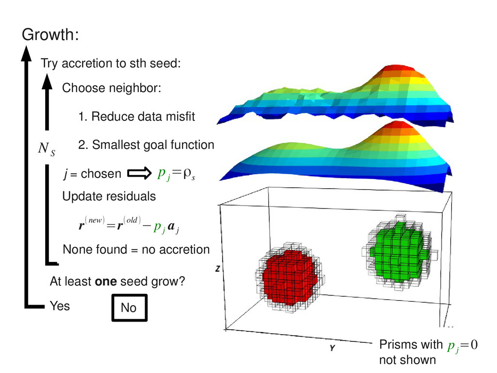
N S Try accretion to sth seed: 1. Reduce data misfit 2. Smallest goal function p j =ρ s j = chosen Update residuals r(new)=r(old )− p j a j Choose neighbor: At least one seed grow? Yes No p j =0
N S Try accretion to sth seed: 1. Reduce data misfit 2. Smallest goal function p j =ρ s j = chosen Update residuals r(new)=r(old )− p j a j Choose neighbor: At least one seed grow? Yes No p j =0
N S Try accretion to sth seed: 1. Reduce data misfit 2. Smallest goal function p j =ρ s j = chosen Update residuals r(new)=r(old )− p j a j Choose neighbor: At least one seed grow? Yes No p j =0 (New elements) j
N S Try accretion to sth seed: 1. Reduce data misfit 2. Smallest goal function p j =ρ s j = chosen Update residuals r(new)=r(old )− p j a j Choose neighbor: At least one seed grow? Yes No p j =0 (New elements) j
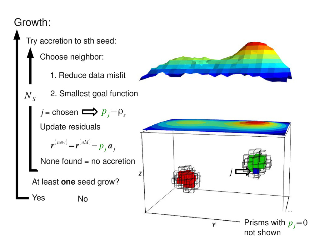
N S Try accretion to sth seed: 1. Reduce data misfit 2. Smallest goal function p j =ρ s j = chosen Update residuals r(new)=r(old )− p j a j Choose neighbor: At least one seed grow? Yes No p j =0 j
N S Try accretion to sth seed: 1. Reduce data misfit 2. Smallest goal function p j =ρ s j = chosen Update residuals r(new)=r(old )− p j a j Choose neighbor: At least one seed grow? Yes No p j =0 j
N S Try accretion to sth seed: 1. Reduce data misfit 2. Smallest goal function p j =ρ s j = chosen Update residuals r(new)=r(old )− p j a j Choose neighbor: At least one seed grow? Yes No p j =0 j
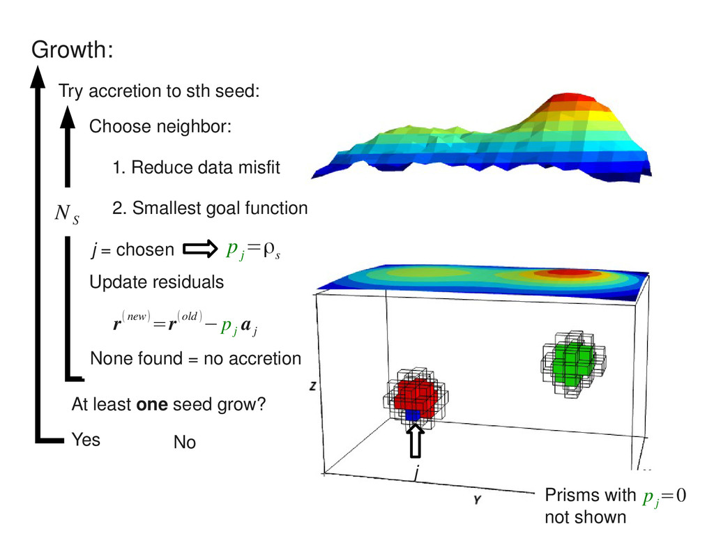
N S Try accretion to sth seed: 1. Reduce data misfit 2. Smallest goal function p j =ρ s j = chosen Update residuals r(new)=r(old )− p j a j Choose neighbor: At least one seed grow? Yes No p j =0 j
N S Try accretion to sth seed: 1. Reduce data misfit 2. Smallest goal function p j =ρ s j = chosen Update residuals r(new)=r(old )− p j a j Choose neighbor: At least one seed grow? Yes No p j =0 j
N S Try accretion to sth seed: 1. Reduce data misfit 2. Smallest goal function p j =ρ s j = chosen Update residuals r(new)=r(old )− p j a j Choose neighbor: At least one seed grow? Yes No p j =0 j
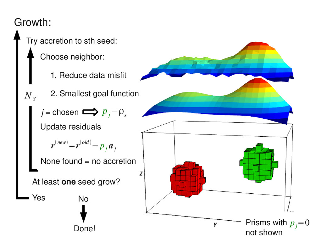
N S Try accretion to sth seed: 1. Reduce data misfit 2. Smallest goal function p j =ρ s j = chosen Update residuals r(new)=r(old )− p j a j Choose neighbor: At least one seed grow? Yes No p j =0
N S Try accretion to sth seed: 1. Reduce data misfit 2. Smallest goal function p j =ρ s j = chosen Update residuals r(new)=r(old )− p j a j Choose neighbor: At least one seed grow? Yes No Done! p j =0
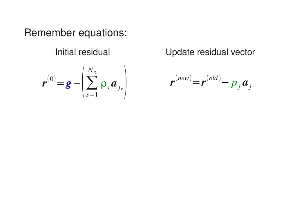
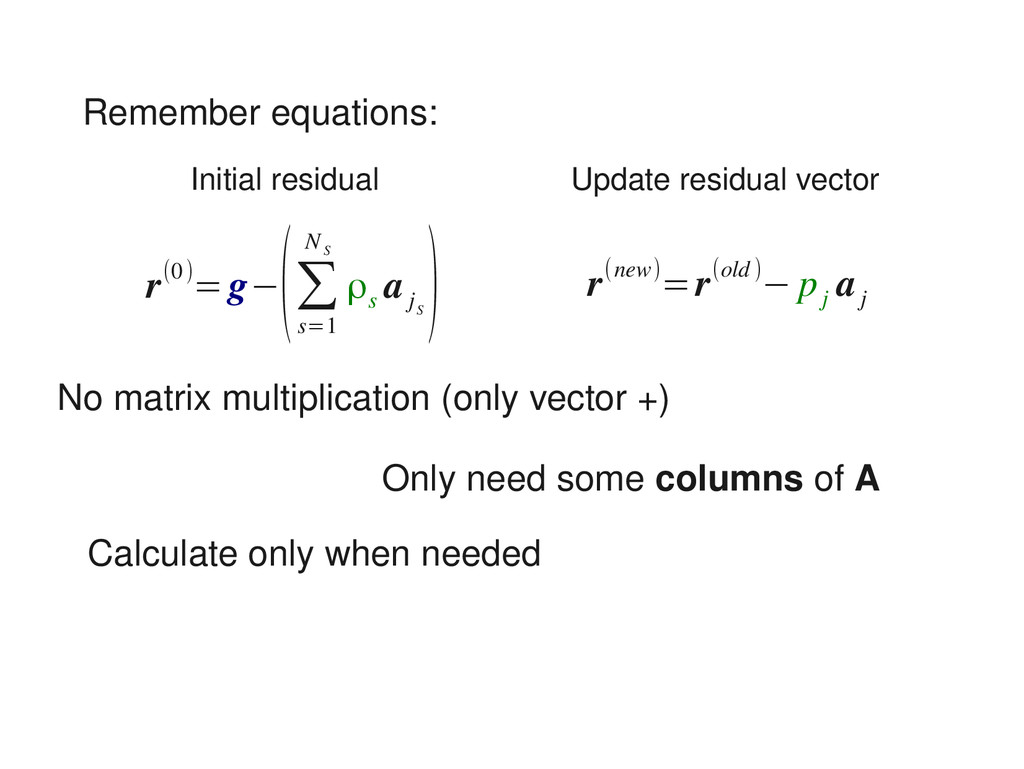
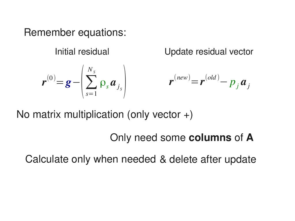
s=1 N S ρ s a j S ) r(new)=r(old)− p j a j Initial residual Update residual vector Only need some columns of A Calculate only when needed & delete after update
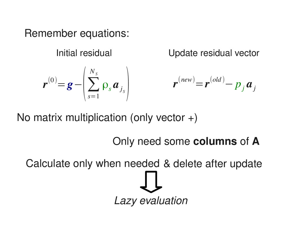
s=1 N S ρ s a j S ) r(new)=r(old)− p j a j Initial residual Update residual vector Only need some columns of A Calculate only when needed Lazy evaluation & delete after update
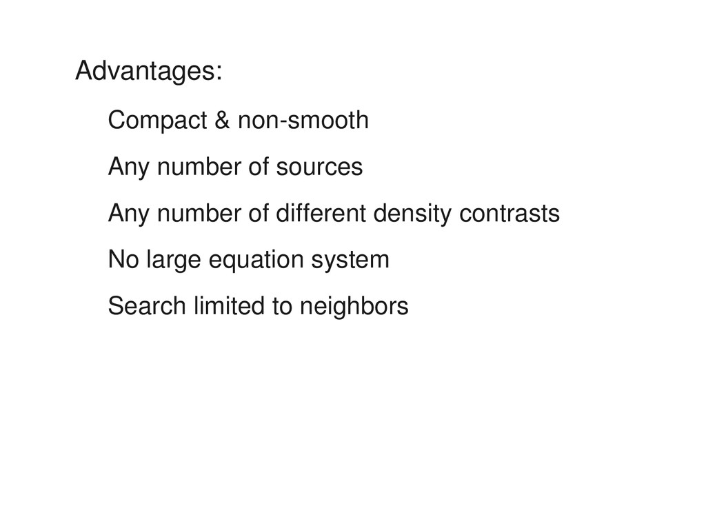
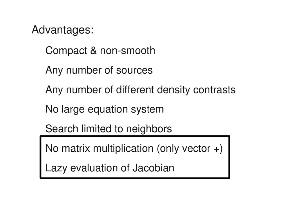
of different density contrasts No large equation system Search limited to neighbors No matrix multiplication (only vector +) Lazy evaluation of Jacobian
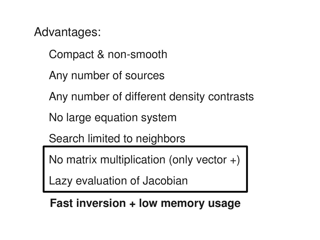
of different density contrasts No large equation system Search limited to neighbors No matrix multiplication (only vector +) Lazy evaluation of Jacobian Fast inversion + low memory usage
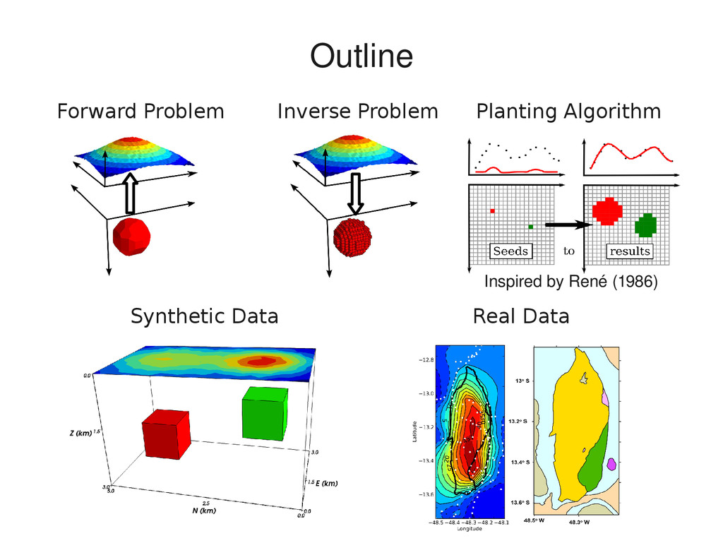
gravitational effects • Abrupt densitycontrast distribution • No matrix multiplication • No need to solve large linear systems • Ideal for: ore bodies, intrusions, salt domes, etc Conclusions