Upgrade to Pro
— share decks privately, control downloads, hide ads and more …
Speaker Deck
Features
Speaker Deck
PRO
Sign in
Sign up for free
Search
Search
3D magnetic inversion by planting anomalous den...
Search
Leonardo Uieda
May 15, 2013
Science
490
1
Share
Embed
Copy iframe code
Copy JS code
Copy link
Start on current slide
3D magnetic inversion by planting anomalous densities
Leonardo Uieda
May 15, 2013
More Decks by Leonardo Uieda
See All by Leonardo Uieda
PhD defense
leouieda
0
1.8k
Inversão gravimétrica do relevo da Moho em coordenadas esféricas
leouieda
0
140
Fatiando a Terra: construindo uma base para ensino e pesquisa de geofísica
leouieda
0
1k
Modelagem e inversão em coordenadas esféricas na gravimetria
leouieda
0
130
Gravity inversion in spherical coordinates using tesseroids
leouieda
0
550
Modelagem gravimétrica em coordenadas esféricas
leouieda
0
170
Iron ore interpretation using gravity-gradient inversions in the Carajás, Brazil
leouieda
0
340
Rapid 3D inversion of gravity and gravity gradient data to test geologic hypotheses
leouieda
1
380
Inversão 3D de campos potenciais em coordenadas esféricas - Parte 1: Modelagem direta
leouieda
2
150
Other Decks in Science
See All in Science
生成AIと司法書士の未来.pdf
tagtag
PRO
0
130
AkarengaLT vol.41
hashimoto_kei
1
150
生成AI・プレプリント時代における 研究成果公開の再設計 ― トップカンファレンス文化はどこへ向かうのか / Redesigning the Dissemination of Research Outputs in the Age of Generative AI and Preprints — Where Is the Top-Conference Culture Heading?
ykiyota
0
29k
データベース09: 実体関連モデル上の一貫性制約
trycycle
PRO
0
1.3k
因果推論と機械学習
sshimizu2006
1
1.2k
医療 LLM ベンチマークの現在地:多面的評価 と日本ローカライズ
analokmaus
1
560
機械学習 - DBSCAN
trycycle
PRO
0
1.9k
Distributional Regression
tackyas
0
550
データベース03: 関係データモデル
trycycle
PRO
1
570
あなたに水耕栽培を愛していないとは言わせない
mutsumix
1
350
ハミルトン・ヤコビ方程式の解の性質と物理的意味
enakai00
0
740
水耕栽培を始める前に知っておきたい植物の科学
grow_design_lab
0
260
Featured
See All Featured
The Web Performance Landscape in 2024 [PerfNow 2024]
tammyeverts
12
1.2k
How Fast Is Fast Enough? [PerfNow 2025]
tammyeverts
3
630
The Curse of the Amulet
leimatthew05
2
13k
Jamie Indigo - Trashchat’s Guide to Black Boxes: Technical SEO Tactics for LLMs
techseoconnect
PRO
0
240
How to Ace a Technical Interview
jacobian
281
24k
Bootstrapping a Software Product
garrettdimon
PRO
307
120k
Mozcon NYC 2025: Stop Losing SEO Traffic
samtorres
1
260
Discover your Explorer Soul
emna__ayadi
2
1.2k
We Are The Robots
honzajavorek
0
260
The Curious Case for Waylosing
cassininazir
1
420
Joys of Absence: A Defence of Solitary Play
codingconduct
1
410
コードの90%をAIが書く世界で何が待っているのか / What awaits us in a world where 90% of the code is written by AI
rkaga
62
44k
Transcript
Leonardo Uieda Valéria C. F. Barbosa Observatório Nacional - Brazil
3D magnetic inversion by planting anomalous densities 2013 AGU Meeting of the Americas
Leonardo Uieda Valéria C. F. Barbosa Observatório Nacional - Brazil
3D magnetic inversion by planting anomalous densities 2013 AGU Meeting of the Americas
Leonardo Uieda Valéria C. F. Barbosa Observatório Nacional - Brazil
3D magnetic inversion by planting anomalous magnetization 2013 AGU Meeting of the Americas
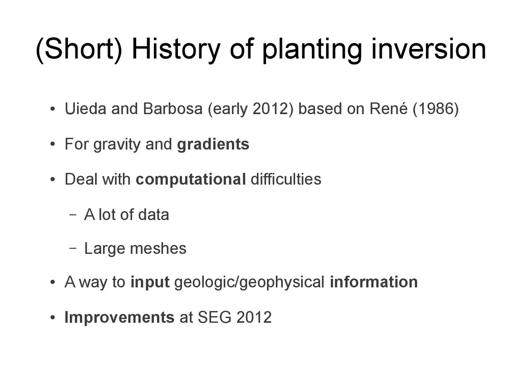
(Short) History of planting inversion • Uieda and Barbosa (early
2012) based on René (1986) • For gravity and gradients • Deal with computational difficulties – A lot of data – Large meshes • A way to input geologic/geophysical information • Improvements at SEG 2012
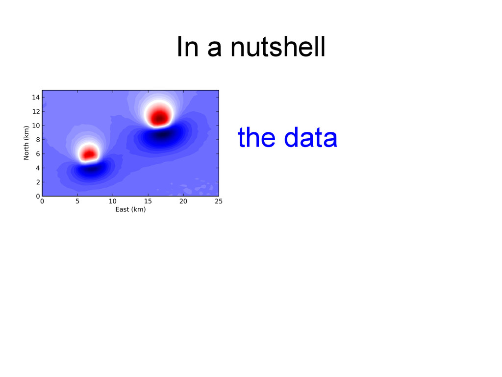
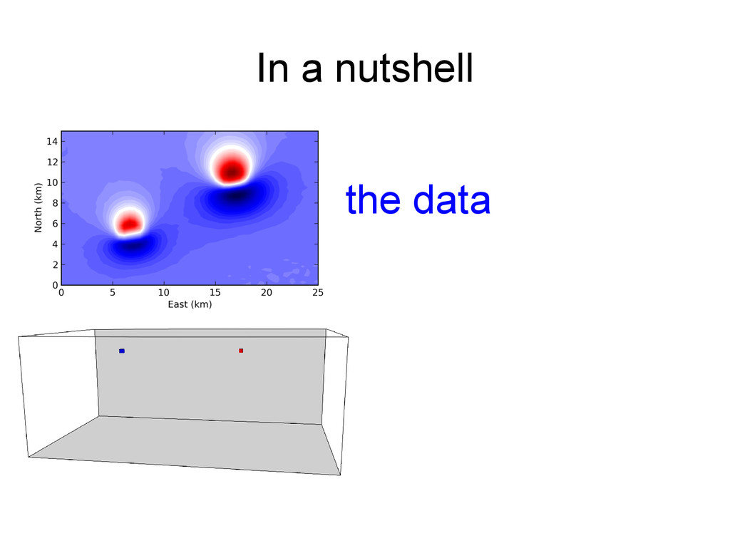
In a nutshell the data
In a nutshell the data
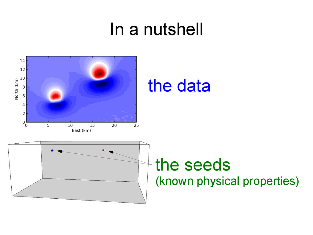
In a nutshell the data the seeds (known physical properties)
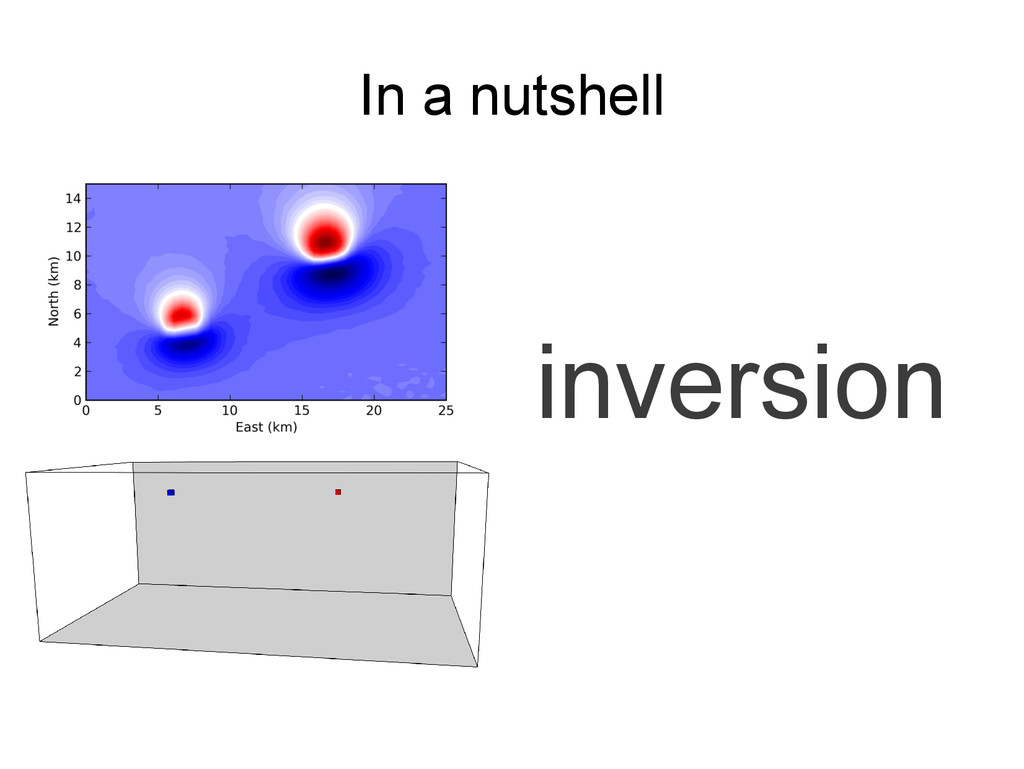
In a nutshell inversion
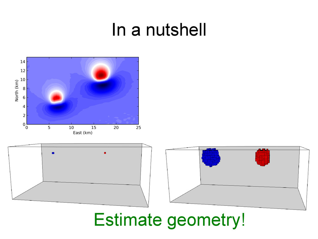
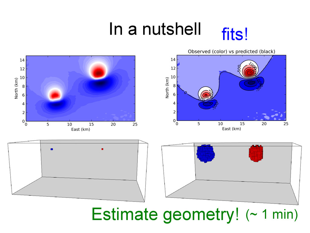
In a nutshell Estimate geometry!
In a nutshell (~ 1 min) Estimate geometry!
In a nutshell fits! (~ 1 min) Estimate geometry!
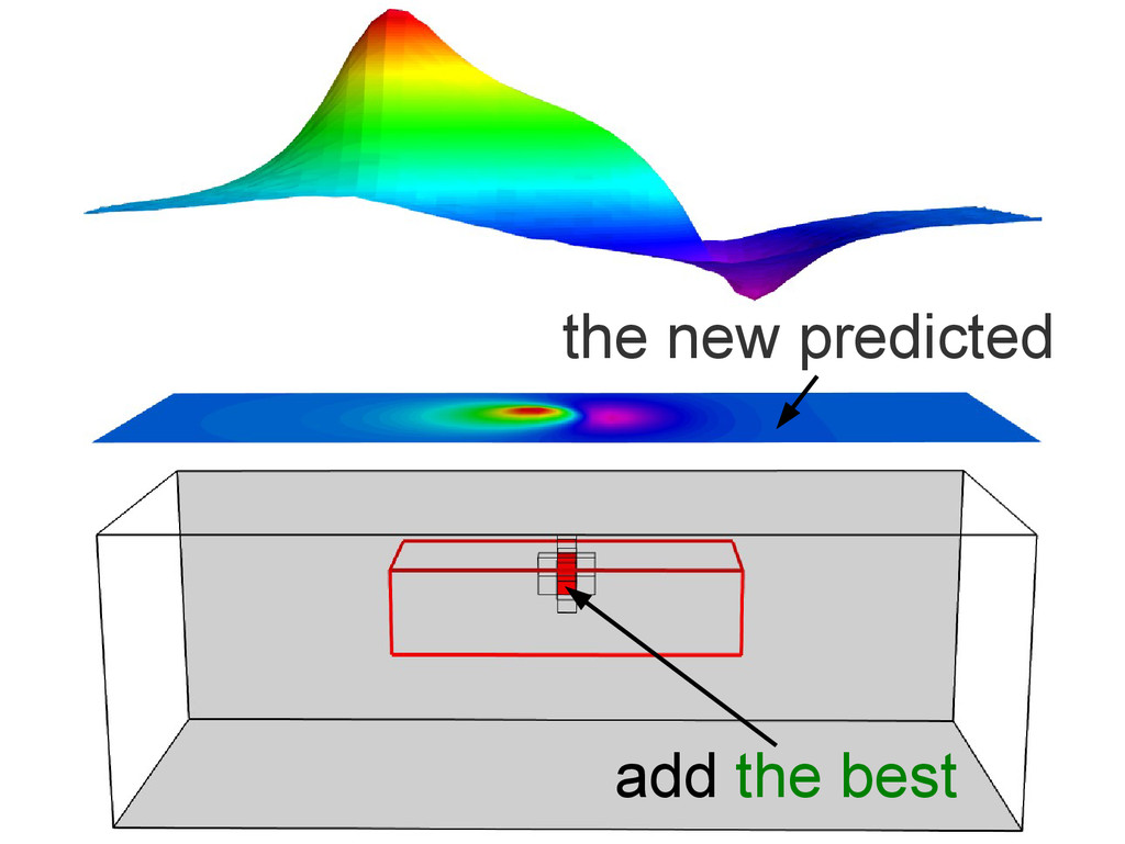
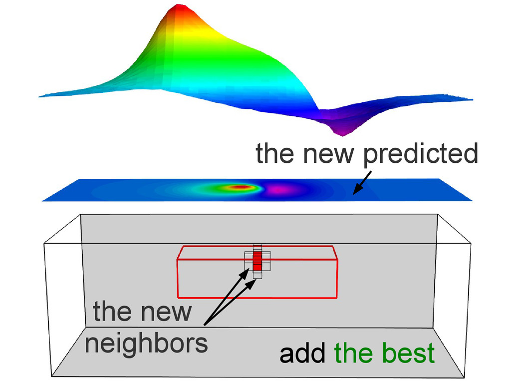
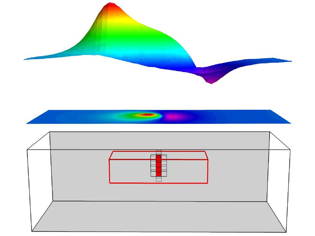
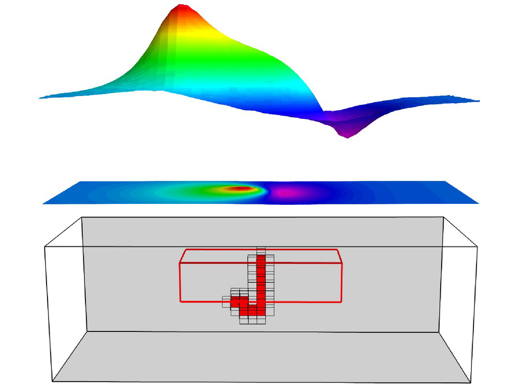
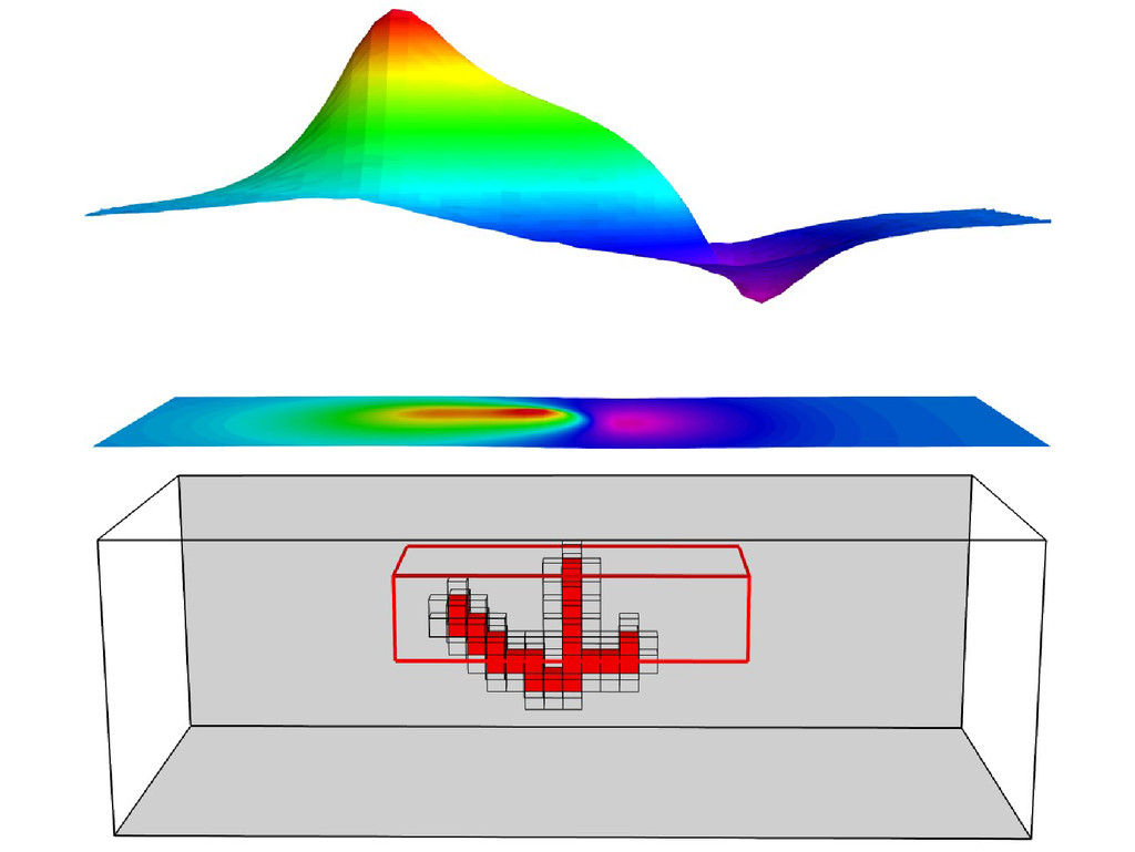
Behind the scenes (aka, Methodology)
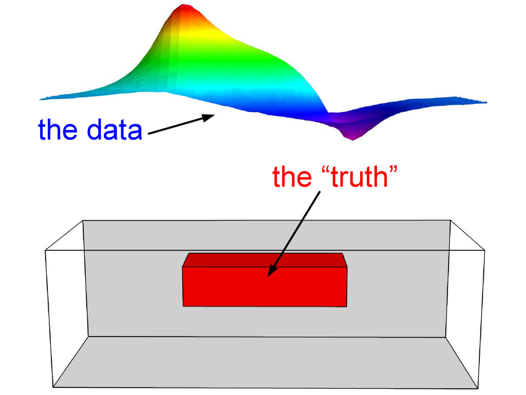
the data the “truth”
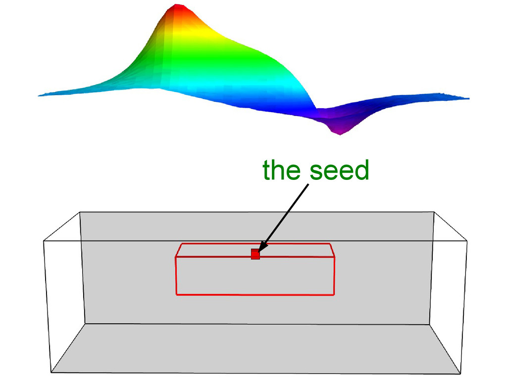
the seed
the predicted data
the neighbors
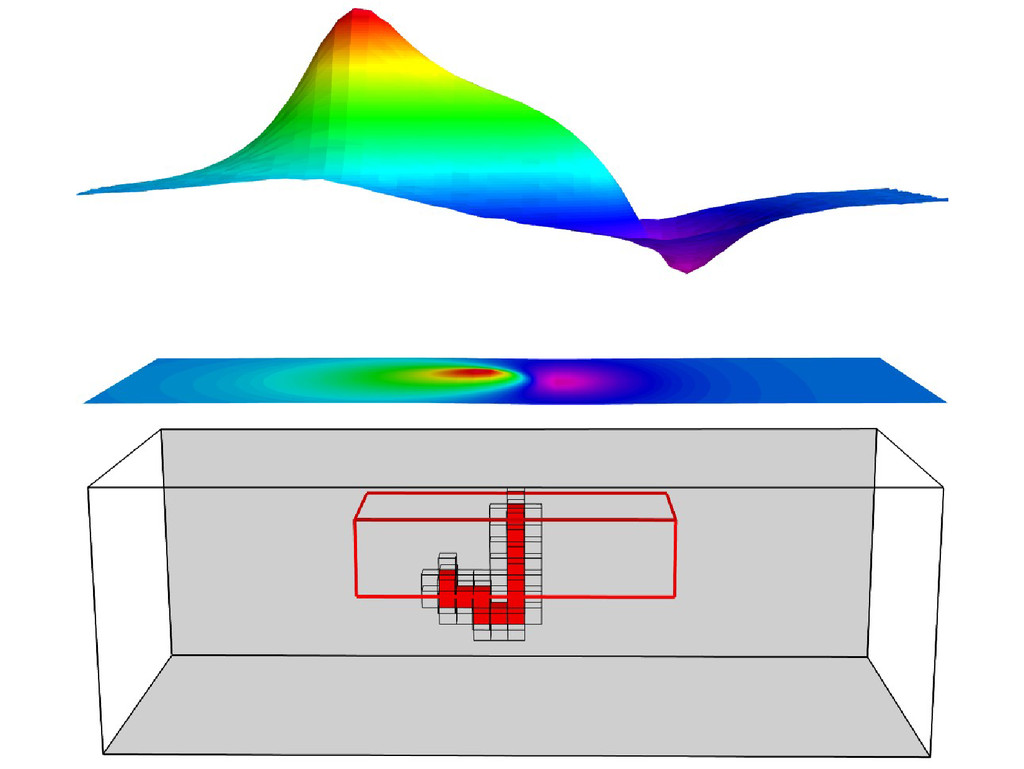
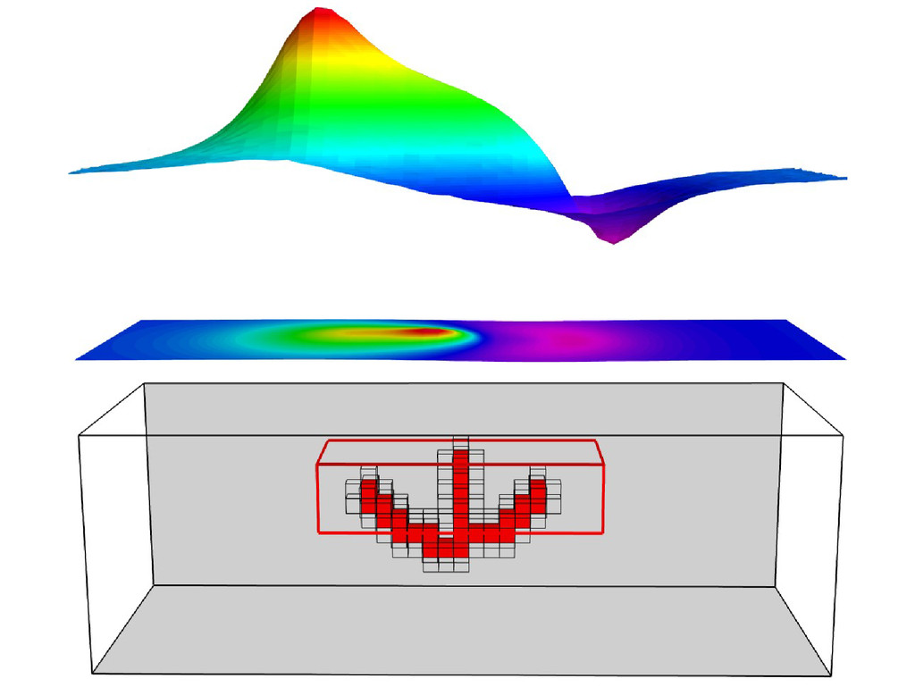
add the best
the new predicted add the best
the new predicted the new neighbors add the best
None
None
None
None
None
None
None
None
None
None
None
None
None
None
None
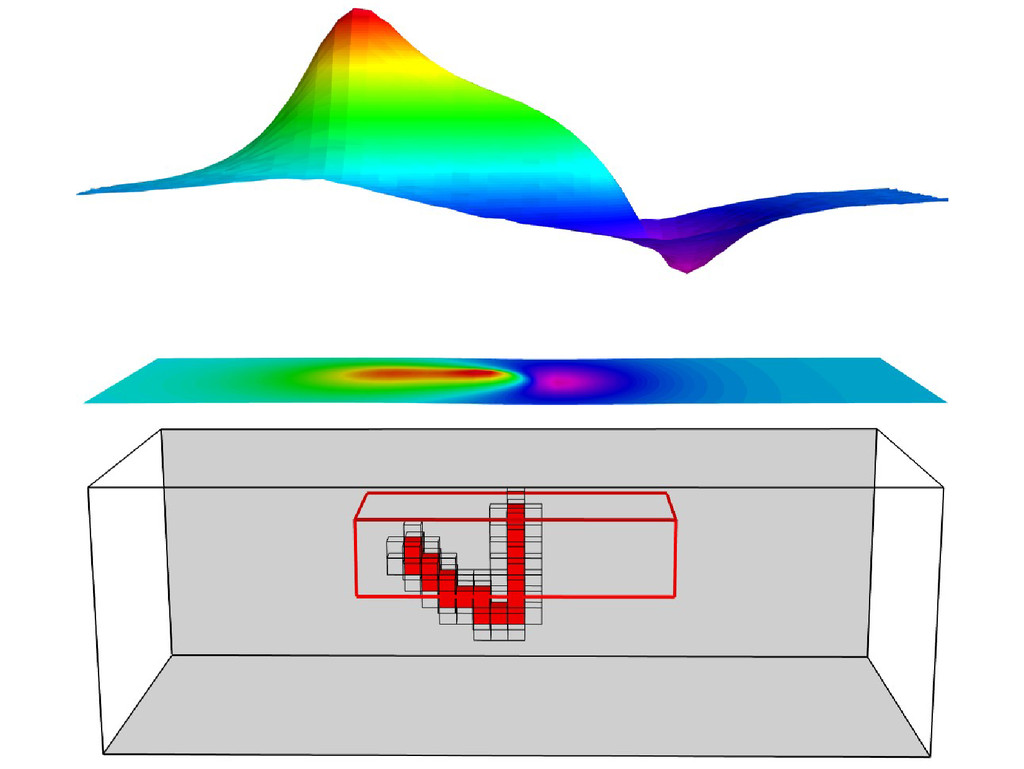
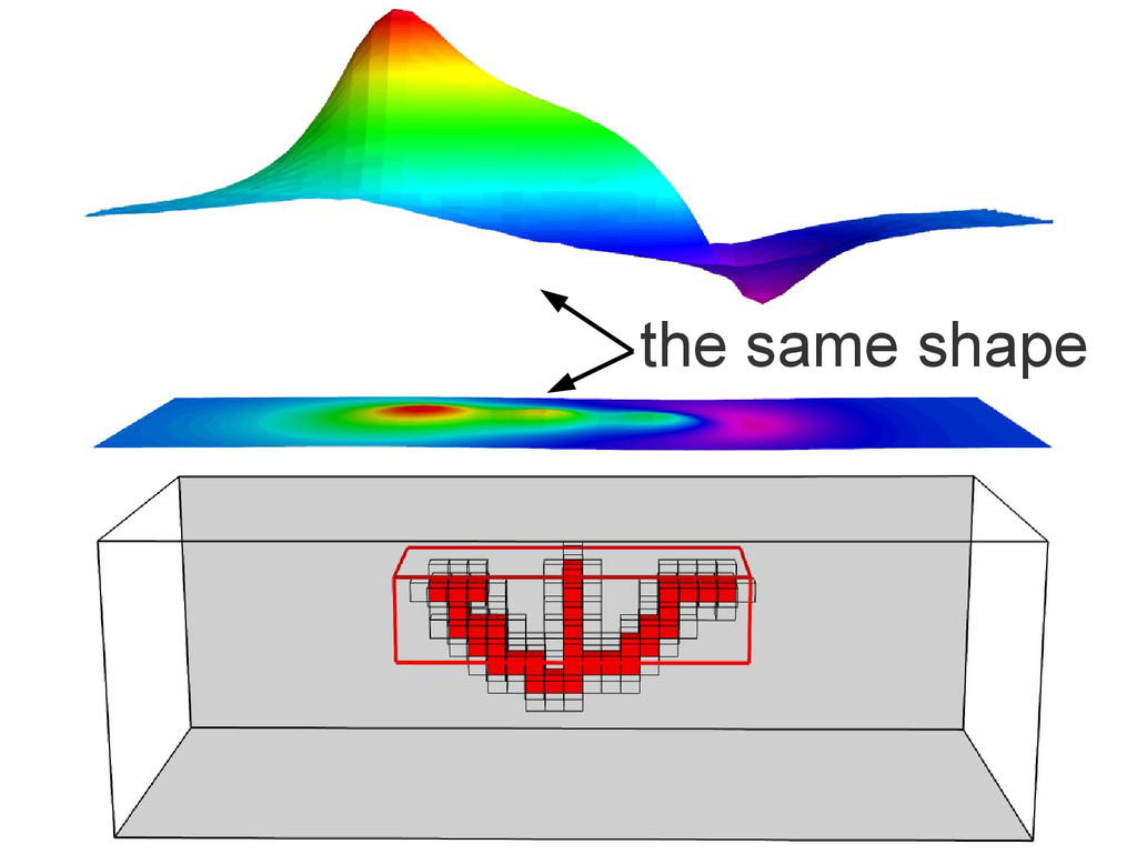
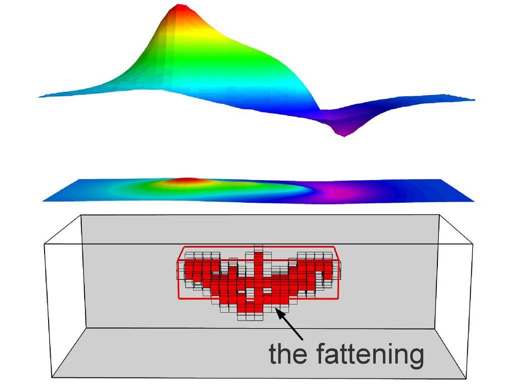
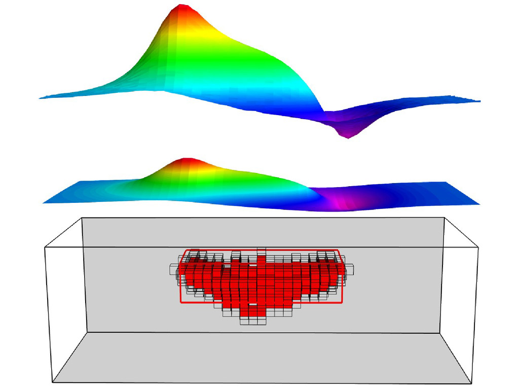
the same shape
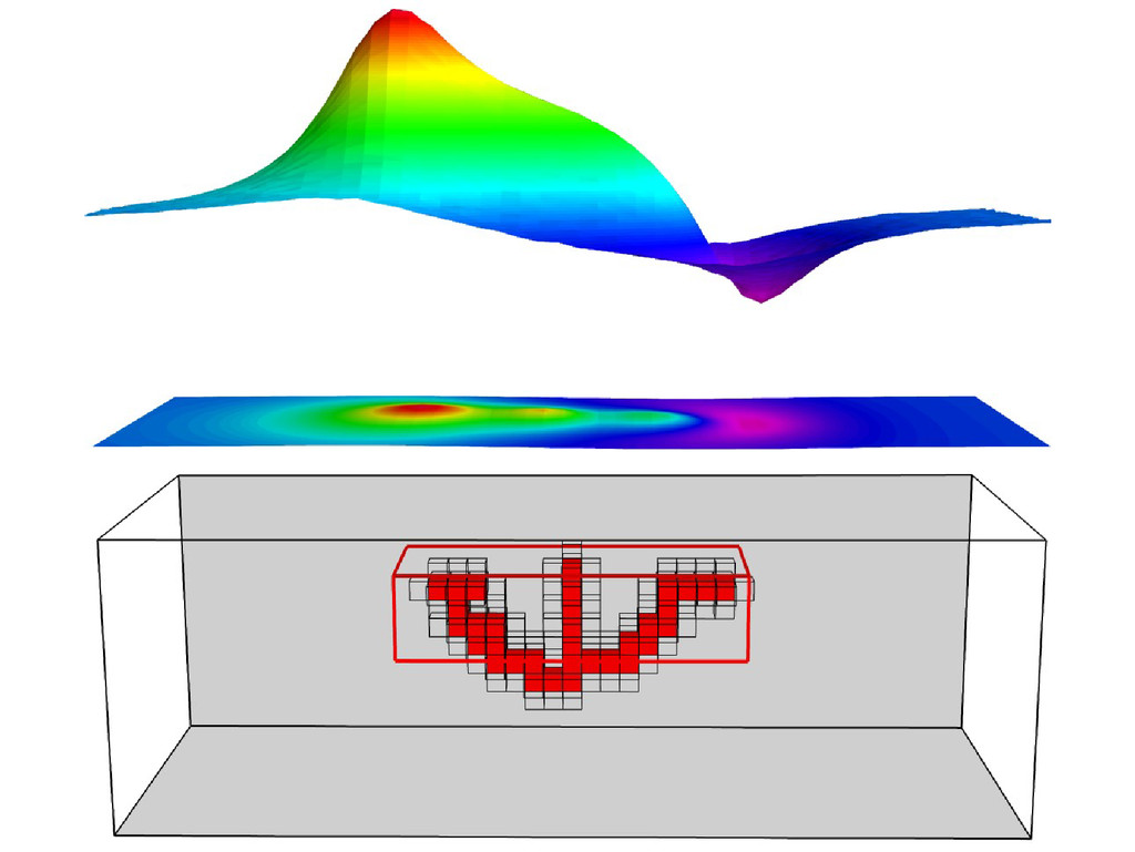
the fattening
the fattening
the fattening
None
None
None
None
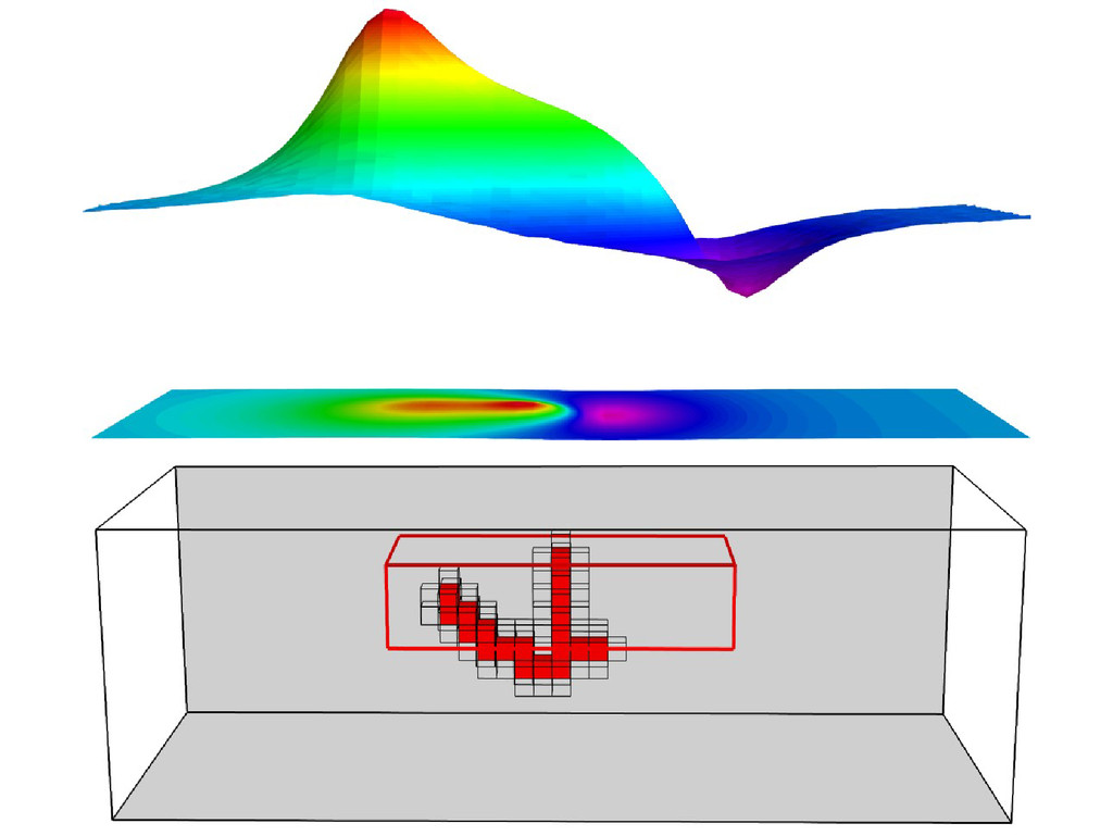
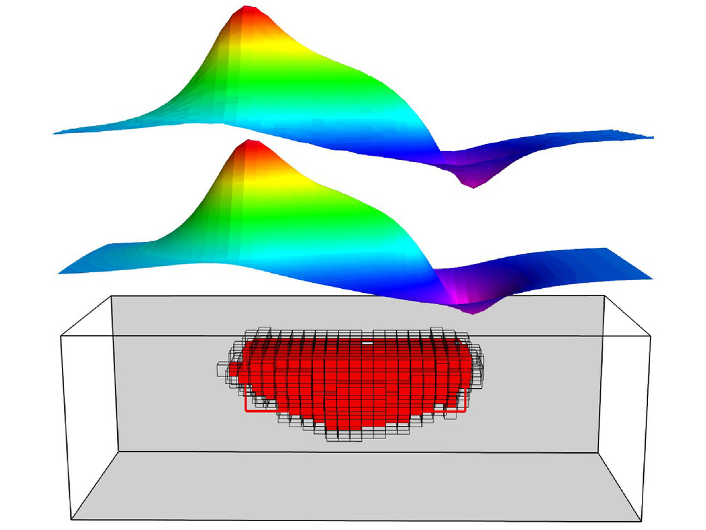
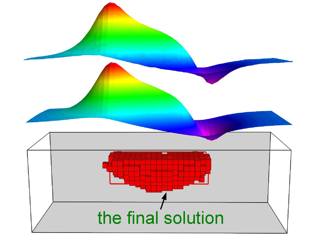
the final solution
the final solution fits!
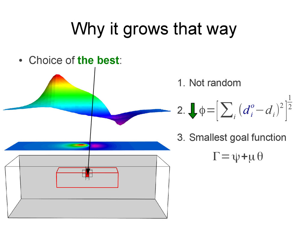
Why it grows that way • Choice of the best:
1. Not random 2. 3. Smallest goal function φ=[∑ i (d i o−d i )2 ]1 2 Γ=ψ+μθ
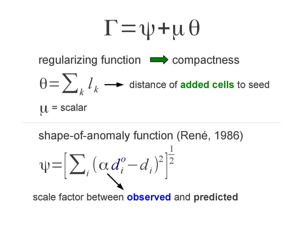
Γ=ψ+μθ θ=∑ k l k regularizing function compactness distance of
added cells to seed = scalar μ
Γ=ψ+μθ θ=∑ k l k regularizing function compactness distance of
added cells to seed ψ=[∑ i (α d i o−d i )2]1 2 shape-of-anomaly function (René, 1986) scale factor between observed and predicted = scalar μ
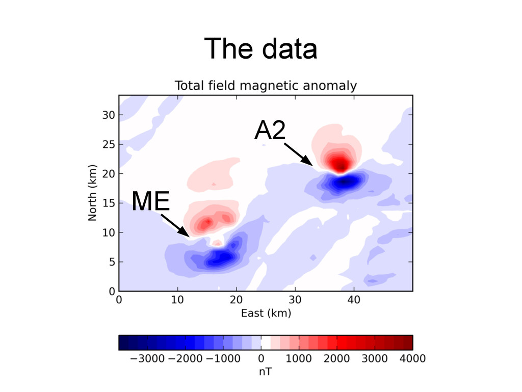
Real data (Morro do Engenho, Brazil)
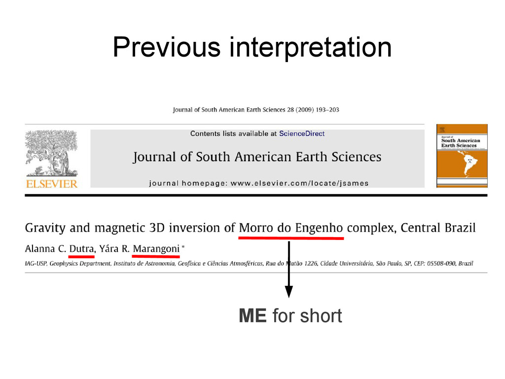
Previous interpretation ME for short
Geologic profile Forward modeling After Dutra and Marangoni (2009) Layered
complex Magnetization Dunite center Know the magnetization
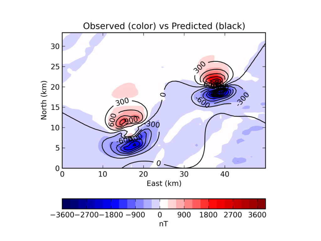
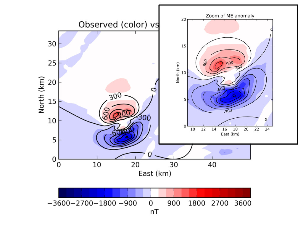
The data
The data ME
The data ME A2
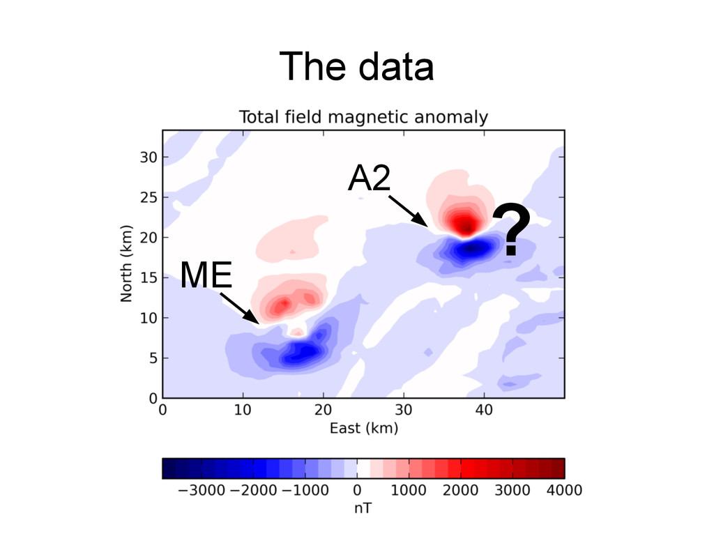
The data ME A2 ?
The data ME A2 ? same as ME?
Test this hypothesis
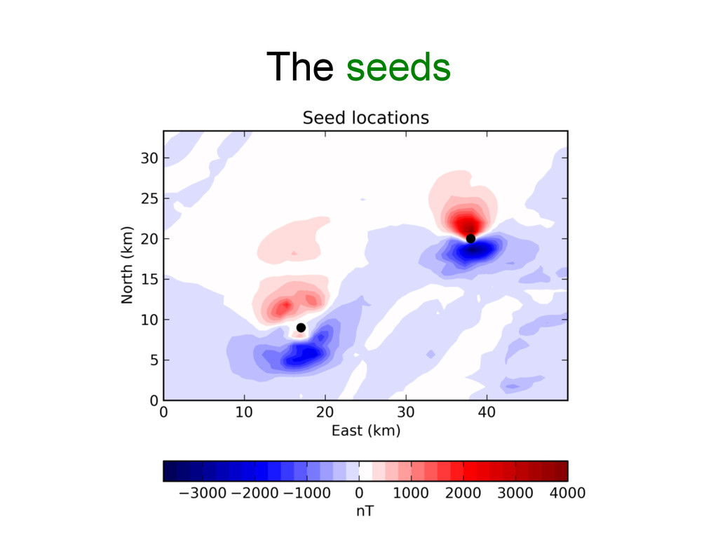
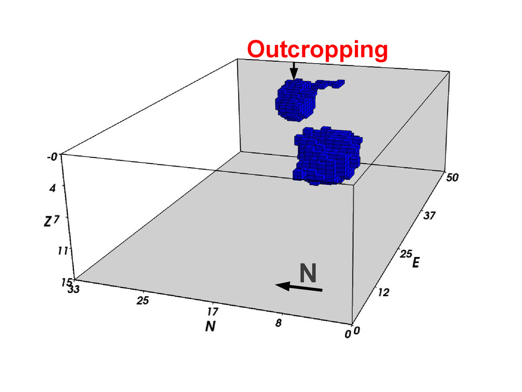
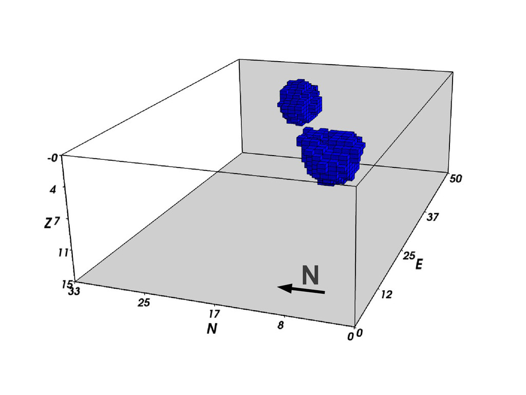
The seeds
N
N
N Outcropping
None
None
None
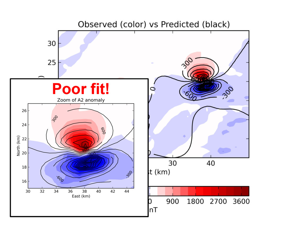
Poor fit!
Get rid of “tentacles”
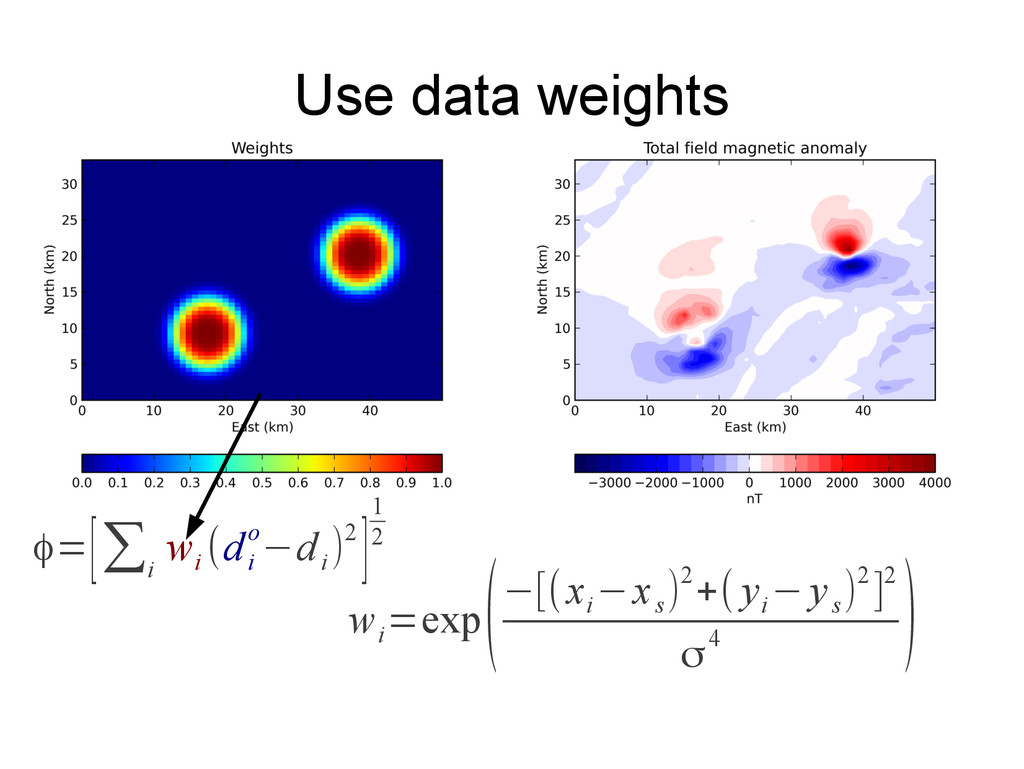
Use data weights
Use data weights φ=[∑ i w i (d i o−d
i )2]1 2
Use data weights φ=[∑ i w i (d i o−d
i )2]1 2 w i =exp (−[(x i −x s )2+( y i −y s )2]2 σ4 )
Use data weights φ=[∑ i w i (d i o−d
i )2]1 2 w i =exp (−[(x i −x s )2+( y i −y s )2]2 σ4 ) s = closest seed
Use data weights φ=[∑ i w i (d i o−d
i )2]1 2 w i =exp (−[(x i −x s )2+( y i −y s )2]2 σ4 ) s = closest seed
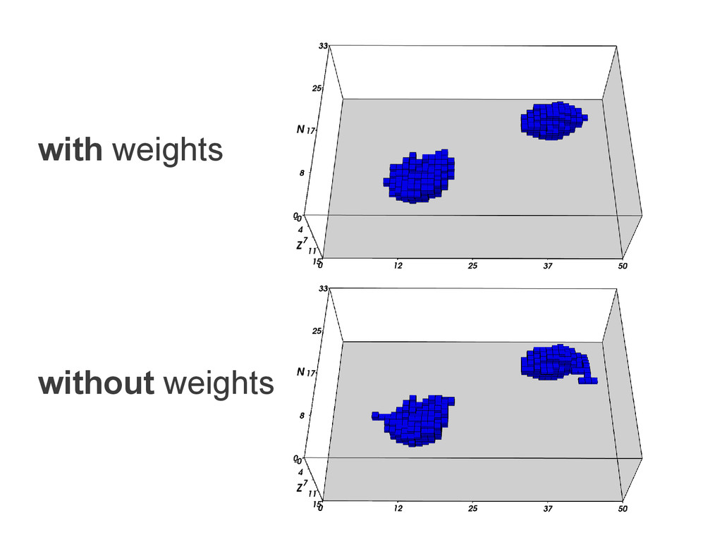
with weights N
N
with weights without weights
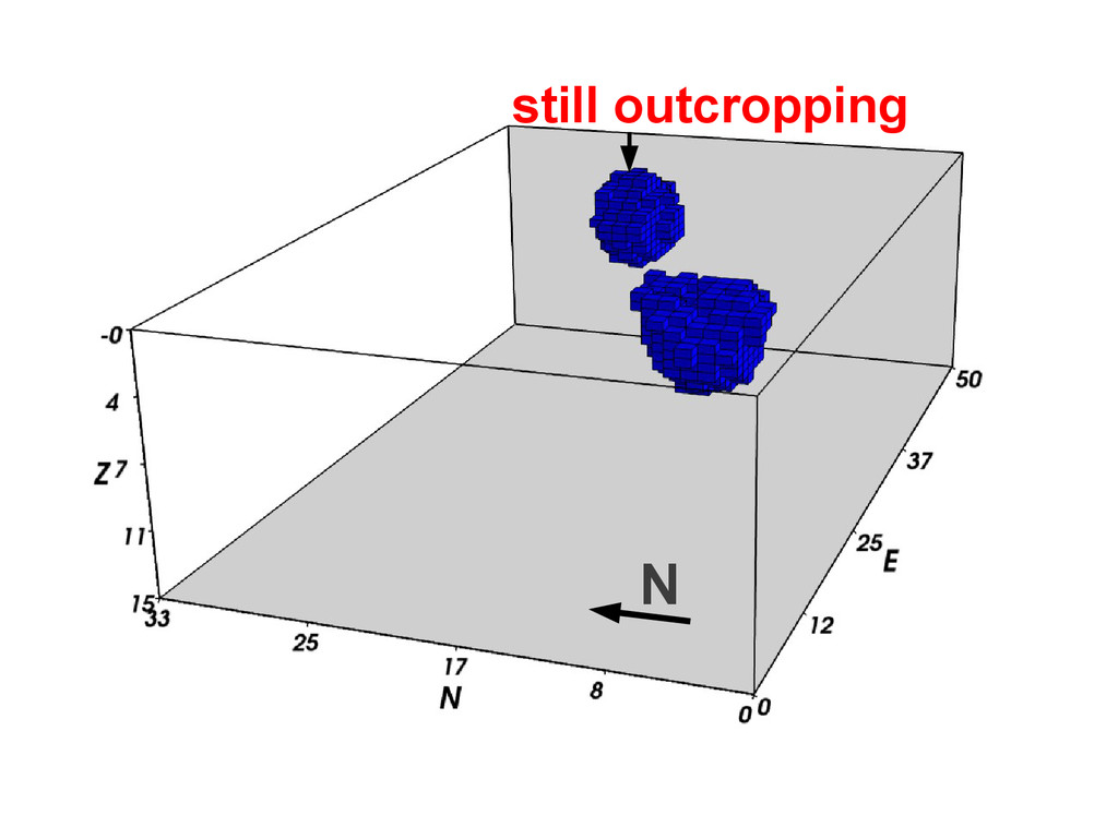
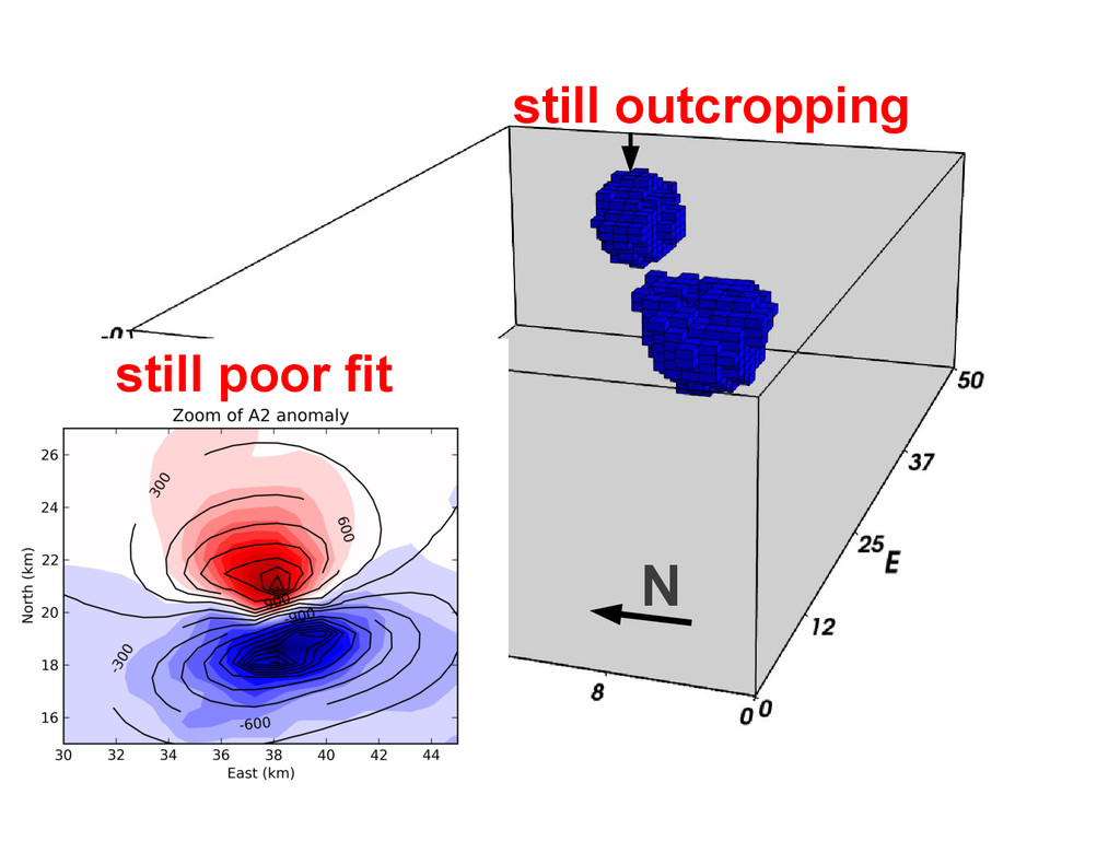
N still outcropping
N still outcropping still poor fit
hypothesis
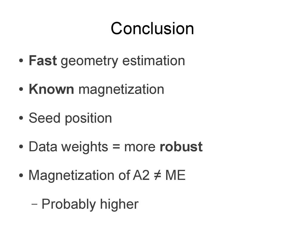
Conclusion • Fast geometry estimation • Known magnetization • Seed
position • Data weights = more robust • Magnetization of A2 ≠ ME – Probably higher
Developed open-source fatiando.org
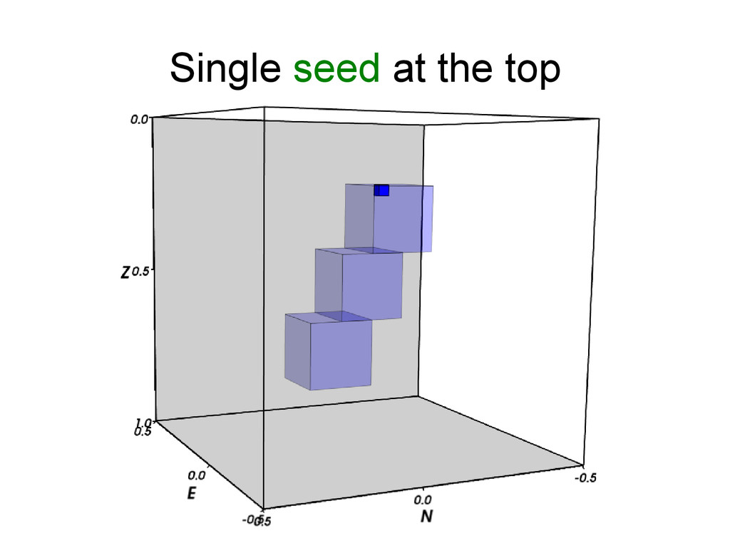
What we're working on (seed positioning)
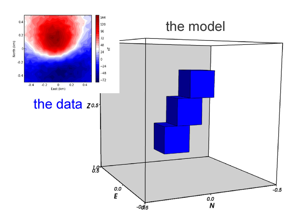
the model the data
Single seed at the top
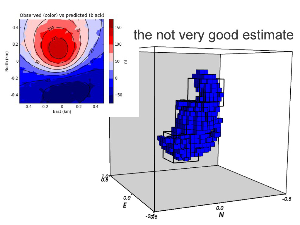
the not very good estimate
the not very good estimate
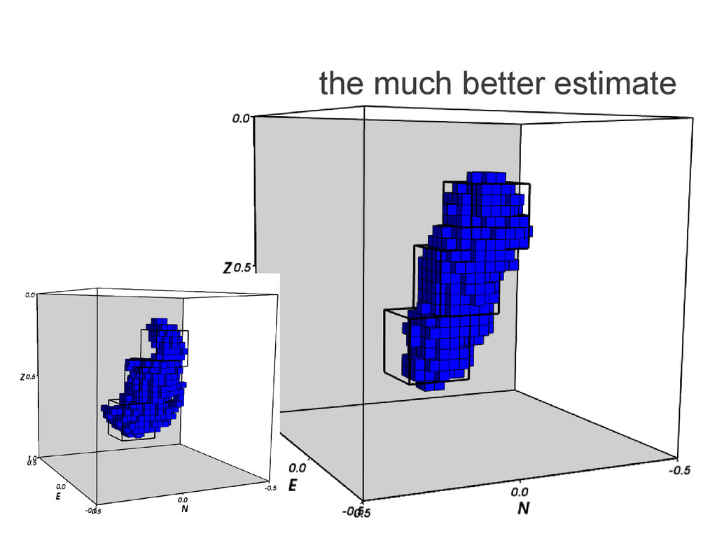
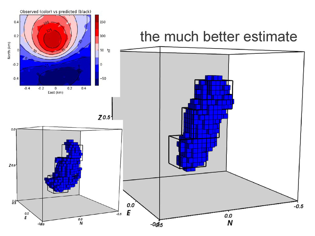
Extract new seeds from estimate
the much better estimate
the much better estimate