L1 Earth Mover's distance

A fast algorithm for Earth Mover's distance

Transcript

1. Fast algorithms for Earth mover’s distance based on optimal transport and L1 regularization Wuchen Li UCLA April 5, 2017 Joint work with Wilfrid Gangbo, Stanley Osher and Penghang Yin. Partially supported by ONR and DOE.
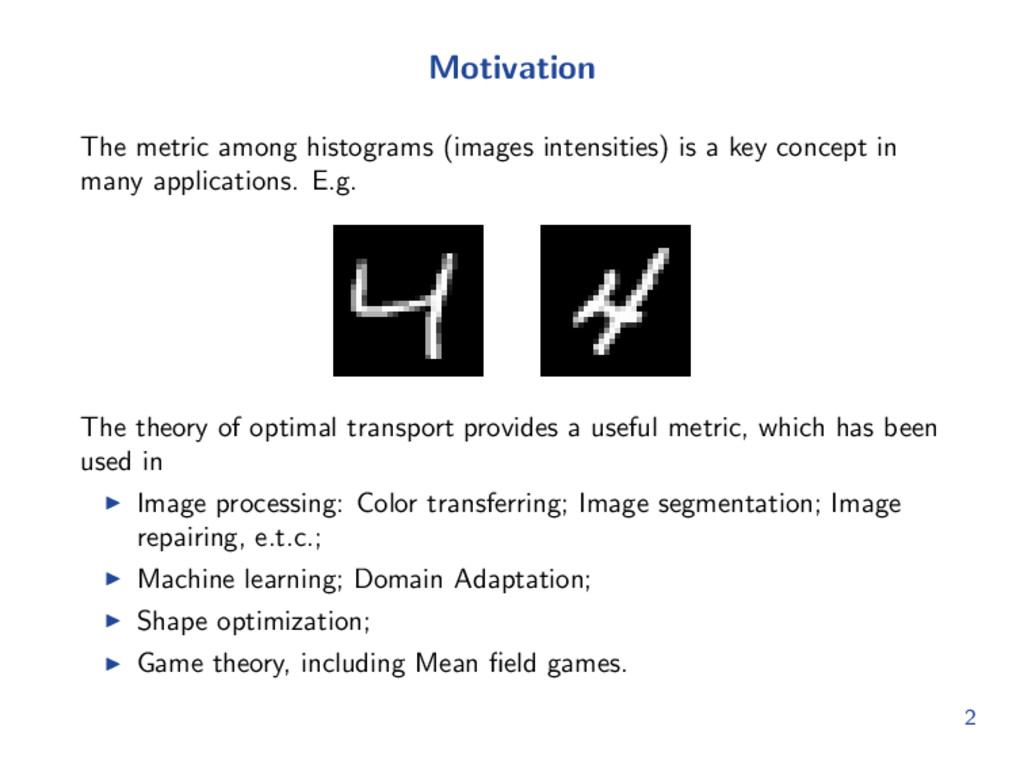
2. Motivation The metric among histograms (images intensities) is a key concept in many applications. E.g. The theory of optimal transport provides a useful metric, which has been used in Image processing: Color transferring; Image segmentation; Image repairing, e.t.c.; Machine learning; Domain Adaptation; Shape optimization; Game theory, including Mean field games. 2
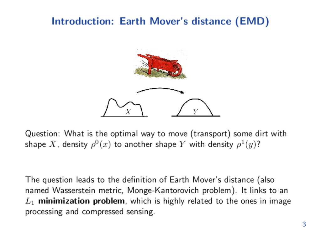
3. Introduction: Earth Mover’s distance (EMD) Question: What is the optimal way to move (transport) some dirt with shape X, density ρ0(x) to another shape Y with density ρ1(y)? The question leads to the definition of Earth Mover’s distance (also named Wasserstein metric, Monge-Kantorovich problem). It links to an L1 minimization problem, which is highly related to the ones in image processing and compressed sensing. 3
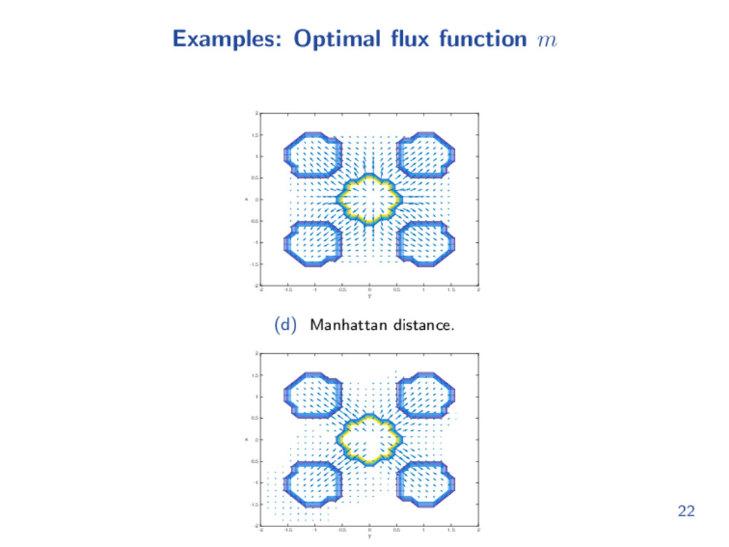
4. Introduction: Problem statement EMD defines a metric on the probability space of a convex, compact set Ω ⊂ Rd: EMD(ρ0, ρ1) := inf π Ω×Ω d(x, y)π(x, y)dxdy where d : Ω × Ω → R is a given cost function, and the infimum is taken among all joint measures having ρ0(x) and ρ1(y) as marginals, i.e. Ω π(x, y)dy = ρ0(x) , Ω π(x, y)dx = ρ1(y) , π(x, y) ≥ 0 . In this talk, we will present fast algorithms for EMD with two different choices of d: d(x, y) = x − y 2 (Euclidean) or x − y 1 (Manhattan) . 4
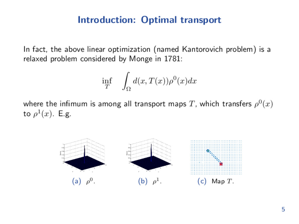
5. Introduction: Optimal transport In fact, the above linear optimization (named Kantorovich problem) is a relaxed problem considered by Monge in 1781: inf T Ω d(x, T(x))ρ0(x)dx where the infimum is among all transport maps T, which transfers ρ0(x) to ρ1(x). E.g. −2 −1 0 1 2 −2 −1 0 1 2 0 0.2 0.4 0.6 0.8 1 x y Density (a) ρ0. −2 −1 0 1 2 −2 −1 0 1 2 0 0.2 0.4 0.6 0.8 1 x y Density (b) ρ1. (c) Map T. 5
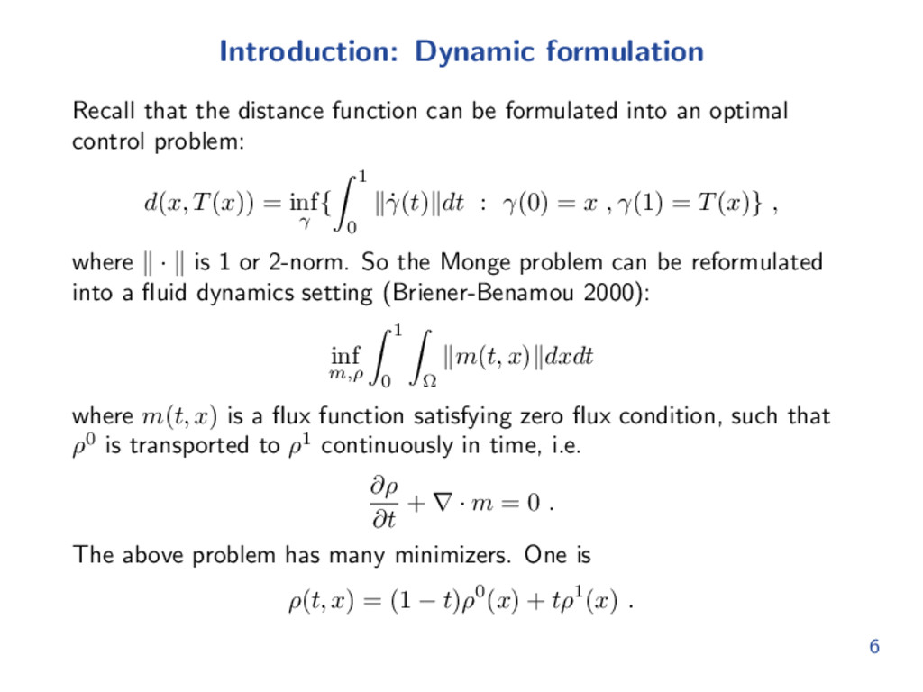
6. Introduction: Dynamic formulation Recall that the distance function can be formulated into an optimal control problem: d(x, T(x)) = inf γ { 1 0 ˙ γ(t) dt : γ(0) = x , γ(1) = T(x)} , where · is 1 or 2-norm. So the Monge problem can be reformulated into a fluid dynamics setting (Briener-Benamou 2000): inf m,ρ 1 0 Ω m(t, x) dxdt where m(t, x) is a flux function satisfying zero flux condition, such that ρ0 is transported to ρ1 continuously in time, i.e. ∂ρ ∂t + ∇ · m = 0 . The above problem has many minimizers. One is ρ(t, x) = (1 − t)ρ0(x) + tρ1(x) . 6
7. Introduction: L1 minimization Thus EMD is equivalent to the following minimal flux formulation: problem: inf m { Ω m(x) dx : ∇ · m(x) + ρ1(x) − ρ0(x) = 0} . It is an L1 minimization, whose minimizer solves the following PDE pairs (Evans and Gangbo 1999)      m(x) = a(x)∇Φ(x) , ∇Φ(x) = 1 , ∇ · (a(x)∇Φ(x)) + ρ1(x) − ρ0(x) = 0 . One may recover the optimal map T by m (under suitable conditions on ρ0 and ρ1): d dt z(t) = m(z) (1 − t)ρ0(z) + tρ1(z) , z(0) = x , z(1) = T(x) . 7
8. L1 minimization From numerical purposes, the minimal flux formulation has two benefits The dimension is much lower than the one in the original linear optimization problem. It is an L1 -type minimization problem, which shares its structure with many problems in compressed sensing and image processing. We borrow a very fast and simple algorithm used there to solve it. 8
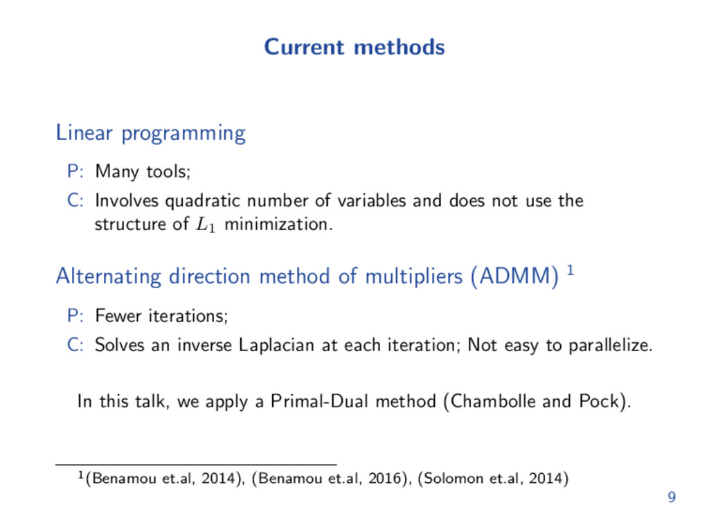
9. Current methods Linear programming P: Many tools; C: Involves quadratic number of variables and does not use the structure of L1 minimization. Alternating direction method of multipliers (ADMM) 1 P: Fewer iterations; C: Solves an inverse Laplacian at each iteration; Not easy to parallelize. In this talk, we apply a Primal-Dual method (Chambolle and Pock). 1(Benamou et.al, 2014), (Benamou et.al, 2016), (Solomon et.al, 2014) 9
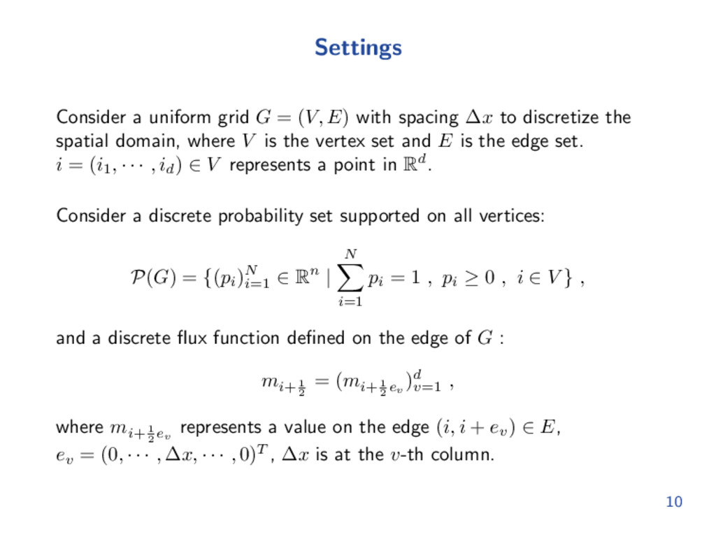
10. Settings Consider a uniform grid G = (V, E) with spacing ∆x to discretize the spatial domain, where V is the vertex set and E is the edge set. i = (i1 , · · · , id ) ∈ V represents a point in Rd. Consider a discrete probability set supported on all vertices: P(G) = {(pi )N i=1 ∈ Rn | N i=1 pi = 1 , pi ≥ 0 , i ∈ V } , and a discrete flux function defined on the edge of G : mi+ 1 2 = (mi+ 1 2 ev )d v=1 , where mi+ 1 2 ev represents a value on the edge (i, i + ev ) ∈ E, ev = (0, · · · , ∆x, · · · , 0)T , ∆x is at the v-th column. 10
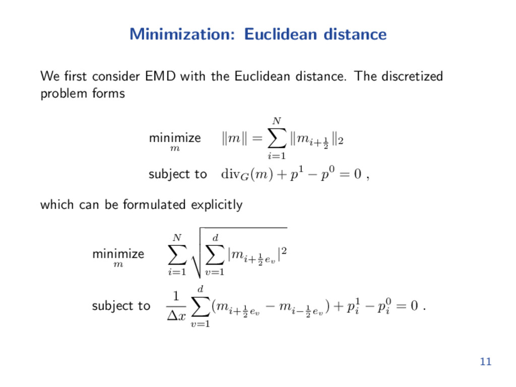
11. Minimization: Euclidean distance We first consider EMD with the Euclidean distance. The discretized problem forms minimize m m = N i=1 mi+ 1 2 2 subject to divG (m) + p1 − p0 = 0 , which can be formulated explicitly minimize m N i=1 d v=1 |mi+ 1 2 ev |2 subject to 1 ∆x d v=1 (mi+ 1 2 ev − mi− 1 2 ev ) + p1 i − p0 i = 0 . 11
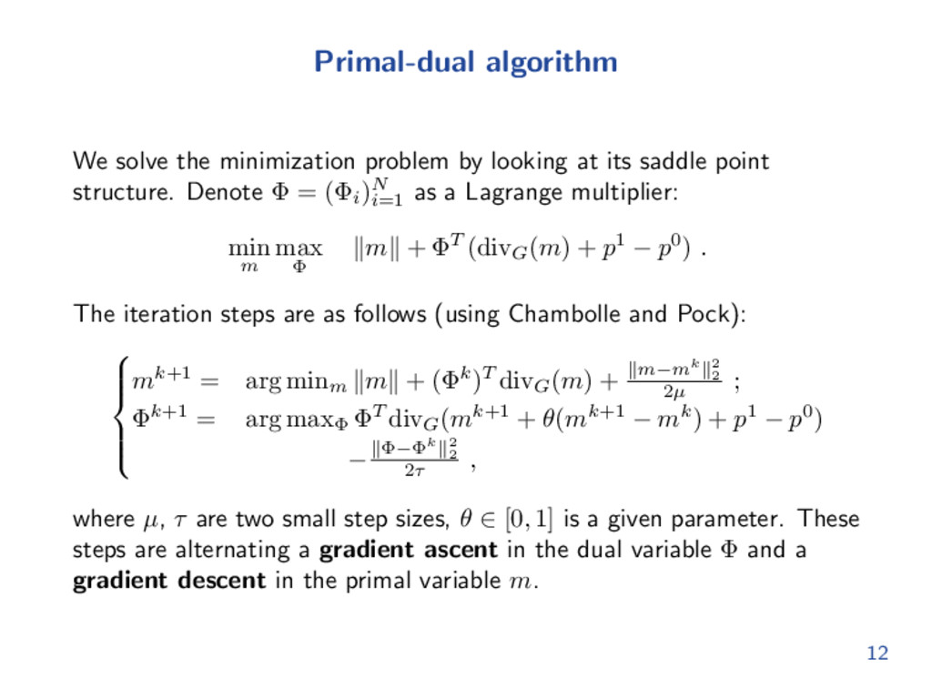
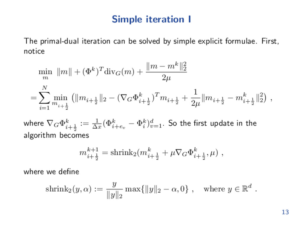
12. Primal-dual algorithm We solve the minimization problem by looking at its saddle point structure. Denote Φ = (Φi )N i=1 as a Lagrange multiplier: min m max Φ m + ΦT (divG (m) + p1 − p0) . The iteration steps are as follows (using Chambolle and Pock):        mk+1 = arg minm m + (Φk)T divG (m) + m−mk 2 2 2µ ; Φk+1 = arg maxΦ ΦT divG (mk+1 + θ(mk+1 − mk) + p1 − p0) − Φ−Φk 2 2 2τ , where µ, τ are two small step sizes, θ ∈ [0, 1] is a given parameter. These steps are alternating a gradient ascent in the dual variable Φ and a gradient descent in the primal variable m. 12
13. Simple iteration I The primal-dual iteration can be solved by simple explicit formulae. First, notice min m m + (Φk)T divG (m) + m − mk 2 2 2µ = N i=1 min m i+ 1 2 mi+ 1 2 2 − (∇G Φk i+ 1 2 )T mi+ 1 2 + 1 2µ mi+ 1 2 − mk i+ 1 2 2 2 , where ∇G Φk i+ 1 2 := 1 ∆x (Φk i+ev − Φk i )d v=1 . So the first update in the algorithm becomes mk+1 i+ 1 2 = shrink2 (mk i+ 1 2 + µ∇G Φk i+ 1 2 , µ) , where we define shrink2 (y, α) := y y 2 max{ y 2 − α, 0} , where y ∈ Rd . 13
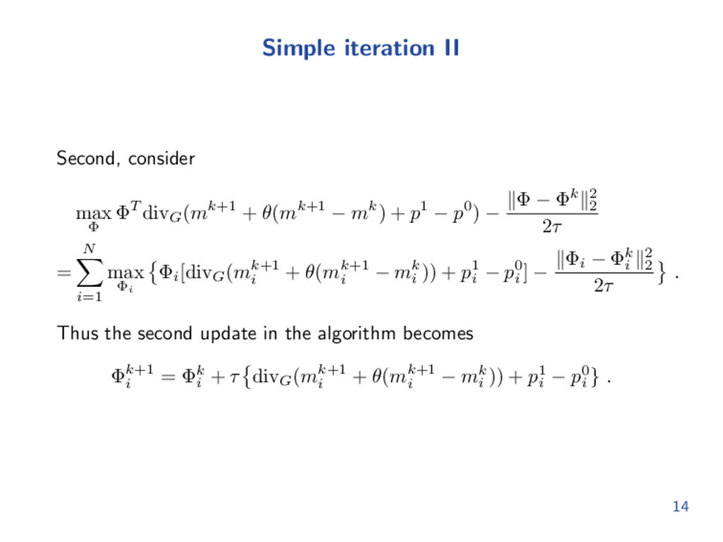
14. Simple iteration II Second, consider max Φ ΦT divG (mk+1 + θ(mk+1 − mk) + p1 − p0) − Φ − Φk 2 2 2τ = N i=1 max Φi Φi [divG (mk+1 i + θ(mk+1 i − mk i )) + p1 i − p0 i ] − Φi − Φk i 2 2 2τ . Thus the second update in the algorithm becomes Φk+1 i = Φk i + τ divG (mk+1 i + θ(mk+1 i − mk i )) + p1 i − p0 i } . 14
15. Algorthim Primal-dual method for EMD-Euclidean metric 1. for k = 1, 2, · · · Iterates until convergence 2. mk+1 i+ 1 2 = shrink2 (mk i+ 1 2 + µ∇G Φk i+ 1 2 , µ) ; 3. Φk+1 i = Φk i + τ{divG (mk+1 i + θ(mk+1 i − mk i )) + p1 i − p0 i } ; 4. End 15
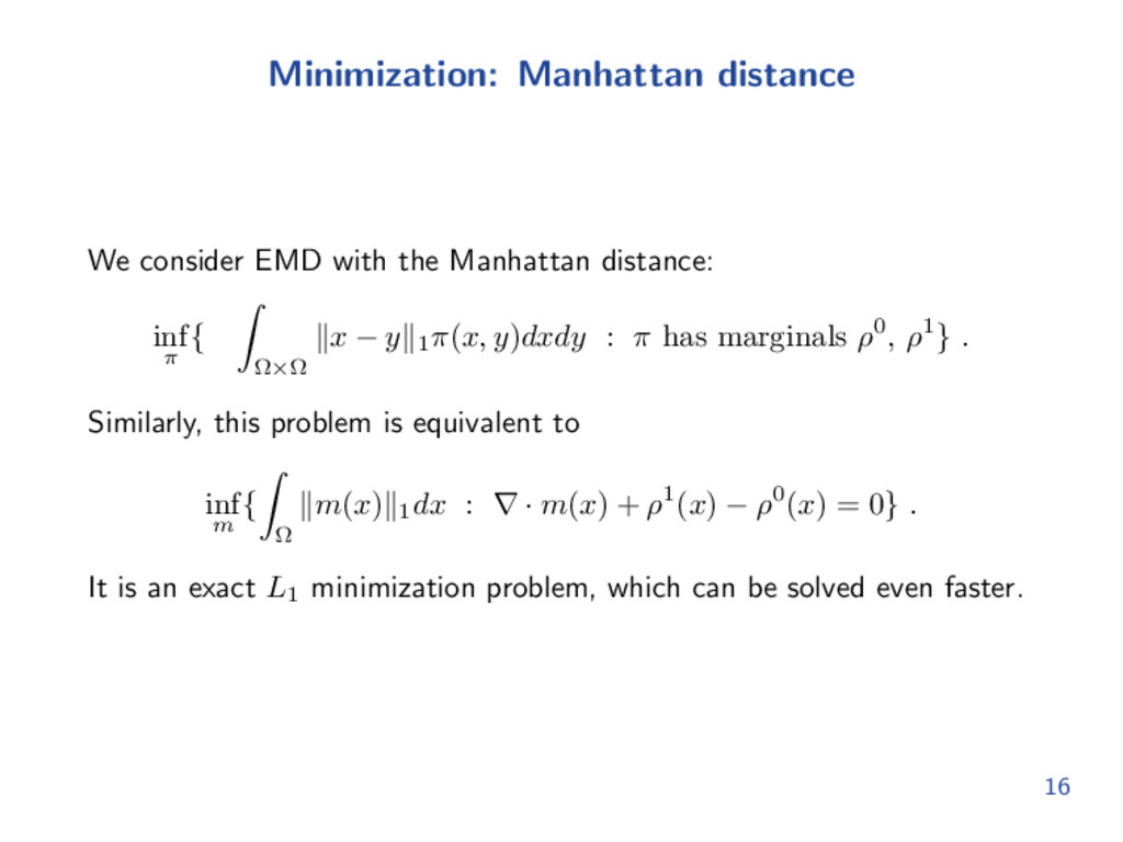
16. Minimization: Manhattan distance We consider EMD with the Manhattan distance: inf π { Ω×Ω x − y 1 π(x, y)dxdy : π has marginals ρ0, ρ1} . Similarly, this problem is equivalent to inf m { Ω m(x) 1 dx : ∇ · m(x) + ρ1(x) − ρ0(x) = 0} . It is an exact L1 minimization problem, which can be solved even faster. 16
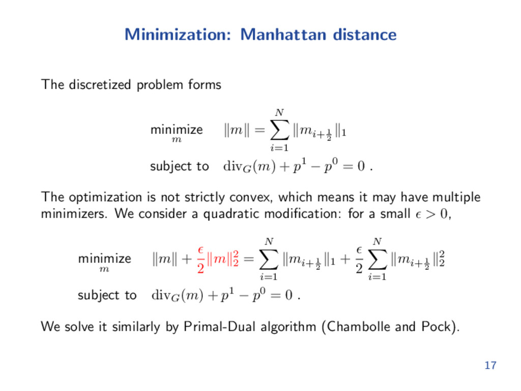
17. Minimization: Manhattan distance The discretized problem forms minimize m m = N i=1 mi+ 1 2 1 subject to divG (m) + p1 − p0 = 0 . The optimization is not strictly convex, which means it may have multiple minimizers. We consider a quadratic modification: for a small > 0, minimize m m + 2 m 2 2 = N i=1 mi+ 1 2 1 + 2 N i=1 mi+ 1 2 2 2 subject to divG (m) + p1 − p0 = 0 . We solve it similarly by Primal-Dual algorithm (Chambolle and Pock). 17
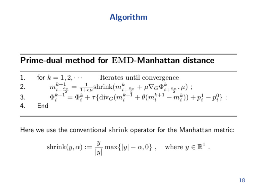
18. Algorithm Prime-dual method for EMD-Manhattan distance 1. for k = 1, 2, · · · Iterates until convergence 2. mk+1 i+ ev 2 = 1 1+ µ shrink(mk i+ ev 2 + µ∇G Φk i+ ev 2 , µ) ; 3. Φk+1 i = Φk i + τ{divG (mk+1 i + θ(mk+1 i − mk i )) + p1 i − p0 i } ; 4. End Here we use the conventional shrink operator for the Manhattan metric: shrink(y, α) := y |y| max{|y| − α, 0} , where y ∈ R1 . 18
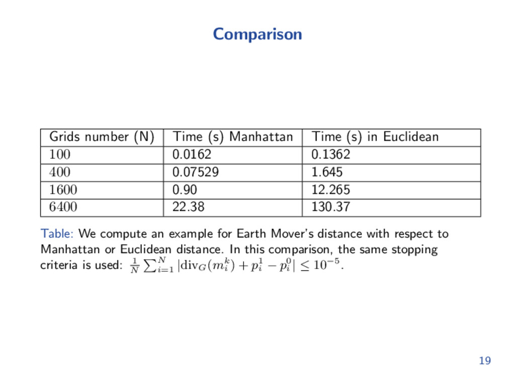
19. Comparison Grids number (N) Time (s) Manhattan Time (s) in Euclidean 100 0.0162 0.1362 400 0.07529 1.645 1600 0.90 12.265 6400 22.38 130.37 Table: We compute an example for Earth Mover’s distance with respect to Manhattan or Euclidean distance. In this comparison, the same stopping criteria is used: 1 N N i=1 |divG (mk i ) + p1 i − p0 i | ≤ 10−5. 19
20. Importance of Grids number N Relative error 400 5.1 × 10−5 1600 6.7 × 10−5 6400 5.3 × 10−4 Table: Computed EMD-Manhattan distance with = 0 and different meshes N. Relative error 0.1 9.1 × 10−4 0.01 9.4 × 10−5 0.001 1.6 × 10−5 0.0001 6.0 × 10−6 Table: Computed EMD-Manhattan distance with a fixed mesh N = 1600 and different . 20
21. Importance of It is worth mentioning that the minimizer of regularized problem inf m { Ω m(x) + 2 m(x) 2dx : ∇ · m(x) + ρ1(x) − ρ0(x) = 0} , satisfies a nice (formal) system m(x) = 1 (∇Φ(x) − ∇Φ(x) |∇Φ(x)| ) , 1 (∆Φ(x) − ∇ · ∇Φ(x) |∇Φ(x)| ) = ρ0(x) − ρ1(x) , where the second equation holds when |∇Φ| ≥ 1. Notice that the term ∇ · ∇Φ(x) |∇Φ(x)| relates to the mean curvature formula. 21
22. Examples: Optimal flux function m y -2 -1.5 -1 -0.5 0 0.5 1 1.5 2 x -2 -1.5 -1 -0.5 0 0.5 1 1.5 2 (d) Manhattan distance. y -2 -1.5 -1 -0.5 0 0.5 1 1.5 2 x -2 -1.5 -1 -0.5 0 0.5 1 1.5 2 22
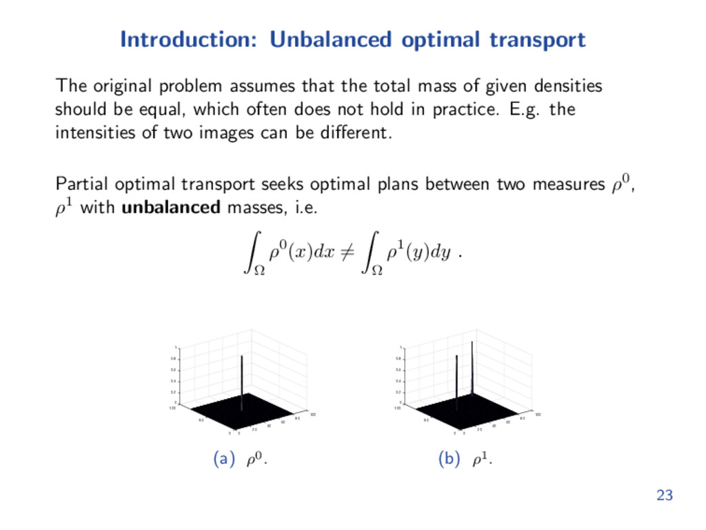
23. Introduction: Unbalanced optimal transport The original problem assumes that the total mass of given densities should be equal, which often does not hold in practice. E.g. the intensities of two images can be different. Partial optimal transport seeks optimal plans between two measures ρ0, ρ1 with unbalanced masses, i.e. Ω ρ0(x)dx = Ω ρ1(y)dy . 100 80 60 40 20 0 0 50 1 0.8 0.6 0.4 0.2 0 100 (a) ρ0. 100 80 60 40 20 0 0 50 1 0 0.2 0.4 0.6 0.8 100 (b) ρ1. 23
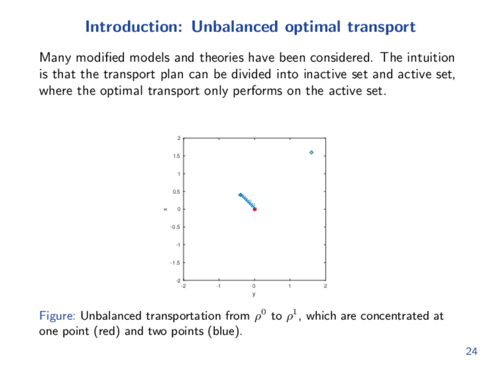
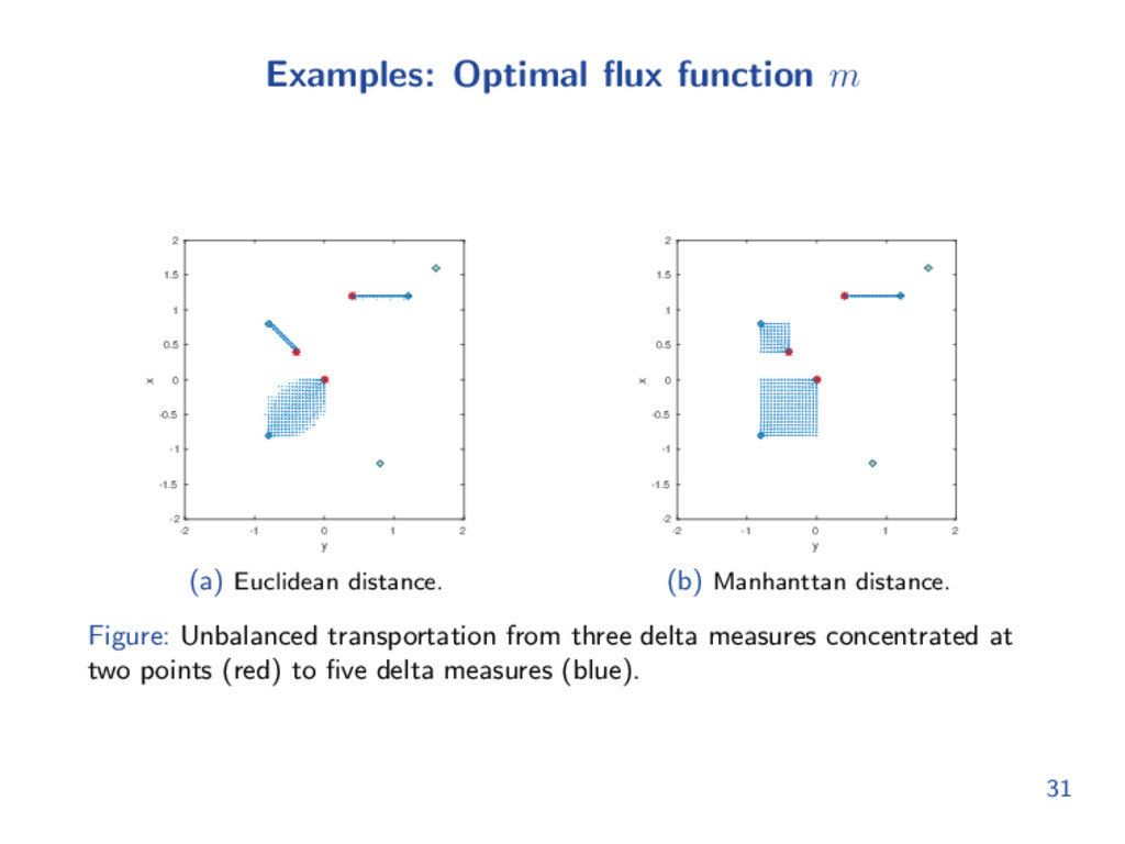
24. Introduction: Unbalanced optimal transport Many modified models and theories have been considered. The intuition is that the transport plan can be divided into inactive set and active set, where the optimal transport only performs on the active set. y -2 -1 0 1 2 x -2 -1.5 -1 -0.5 0 0.5 1 1.5 2 Figure: Unbalanced transportation from ρ0 to ρ1, which are concentrated at one point (red) and two points (blue). 24
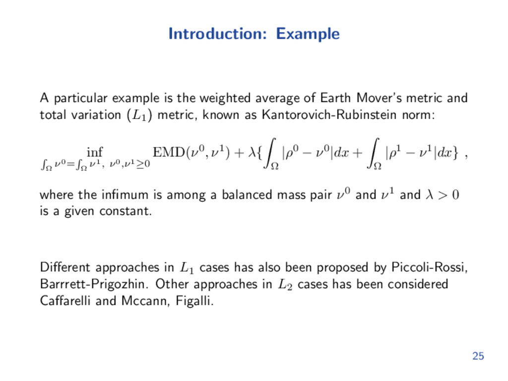
25. Introduction: Example A particular example is the weighted average of Earth Mover’s metric and total variation (L1 ) metric, known as Kantorovich-Rubinstein norm: inf Ω ν0= Ω ν1, ν0,ν1≥0 EMD(ν0, ν1) + λ{ Ω |ρ0 − ν0|dx + Ω |ρ1 − ν1|dx} , where the infimum is among a balanced mass pair ν0 and ν1 and λ > 0 is a given constant. Different approaches in L1 cases has also been proposed by Piccoli-Rossi, Barrrett-Prigozhin. Other approaches in L2 cases has been considered Caffarelli and Mccann, Figalli. 25
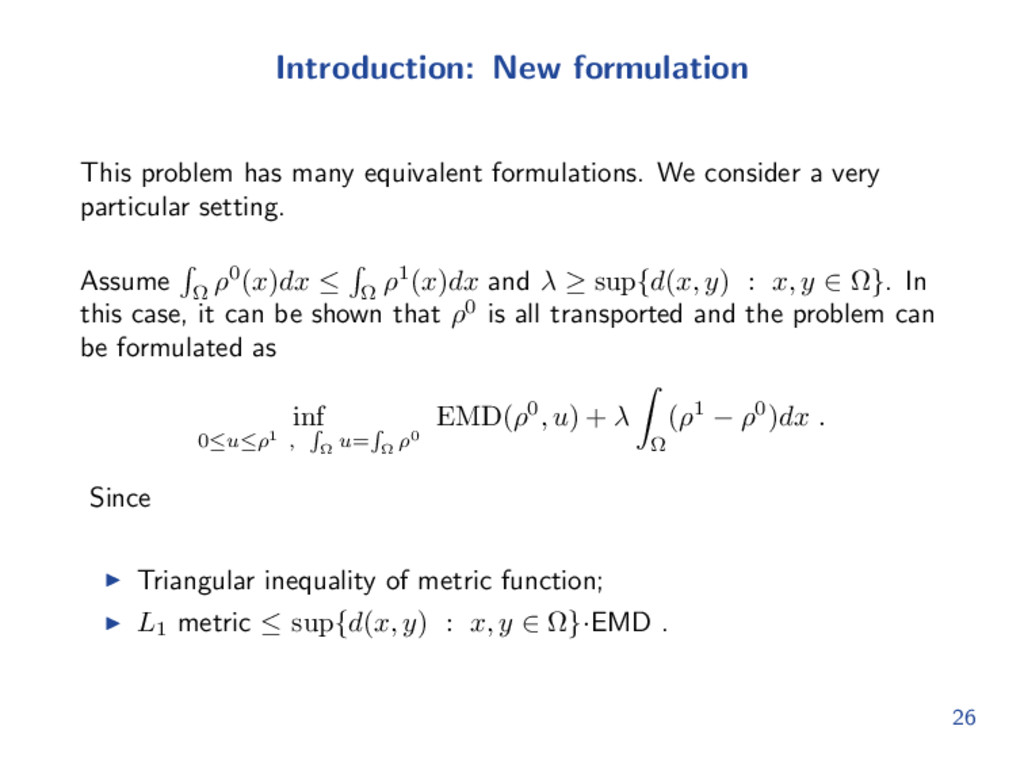
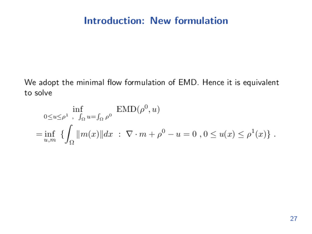
26. Introduction: New formulation This problem has many equivalent formulations. We consider a very particular setting. Assume Ω ρ0(x)dx ≤ Ω ρ1(x)dx and λ ≥ sup{d(x, y) : x, y ∈ Ω}. In this case, it can be shown that ρ0 is all transported and the problem can be formulated as inf 0≤u≤ρ1 , Ω u= Ω ρ0 EMD(ρ0, u) + λ Ω (ρ1 − ρ0)dx . Since Triangular inequality of metric function; L1 metric ≤ sup{d(x, y) : x, y ∈ Ω}·EMD . 26
27. Introduction: New formulation We adopt the minimal flow formulation of EMD. Hence it is equivalent to solve inf 0≤u≤ρ1 , Ω u= Ω ρ0 EMD(ρ0, u) = inf u,m { Ω m(x) dx : ∇ · m + ρ0 − u = 0 , 0 ≤ u(x) ≤ ρ1(x)} . 27
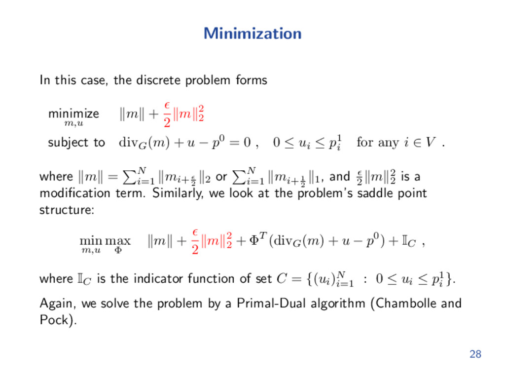
28. Minimization In this case, the discrete problem forms minimize m,u m + 2 m 2 2 subject to divG (m) + u − p0 = 0 , 0 ≤ ui ≤ p1 i for any i ∈ V . where m = N i=1 mi+ 2 2 or N i=1 mi+ 1 2 1 , and 2 m 2 2 is a modification term. Similarly, we look at the problem’s saddle point structure: min m,u max Φ m + 2 m 2 2 + ΦT (divG (m) + u − p0) + IC , where IC is the indicator function of set C = {(ui )N i=1 : 0 ≤ ui ≤ p1 i }. Again, we solve the problem by a Primal-Dual algorithm (Chambolle and Pock). 28
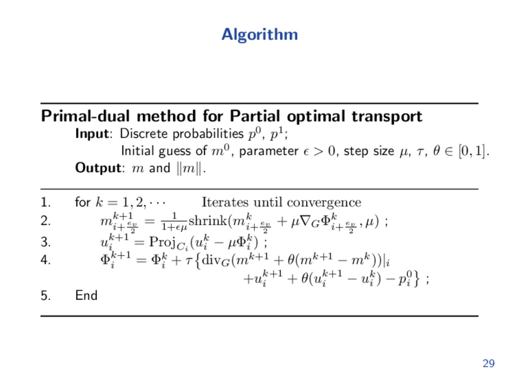
29. Algorithm Primal-dual method for Partial optimal transport Input: Discrete probabilities p0, p1; Initial guess of m0, parameter > 0, step size µ, τ, θ ∈ [0, 1]. Output: m and m . 1. for k = 1, 2, · · · Iterates until convergence 2. mk+1 i+ ev 2 = 1 1+ µ shrink(mk i+ ev 2 + µ∇G Φk i+ ev 2 , µ) ; 3. uk+1 i = ProjCi (uk i − µΦk i ) ; 4. Φk+1 i = Φk i + τ divG (mk+1 + θ(mk+1 − mk))|i +uk+1 i + θ(uk+1 i − uk i ) − p0 i ; 5. End 29
30. Examples 0.9579 1.0257 1.2310 2.2570 2.6128 2.9389 3.9246 Figure: Hand written digit images and the computed distances between the top left image and the rest. 30
31. Examples: Optimal flux function m y -2 -1 0 1 2 x -2 -1.5 -1 -0.5 0 0.5 1 1.5 2 (a) Euclidean distance. y -2 -1 0 1 2 x -2 -1.5 -1 -0.5 0 0.5 1 1.5 2 (b) Manhanttan distance. Figure: Unbalanced transportation from three delta measures concentrated at two points (red) to five delta measures (blue). 31
32. Discussion We conclude that the algorithm can handle the sparsity of EMD; have simple updates; be easy to parallelize; be regularized efficiently in the Manhattan metric case by adding 2 m 2 2 . 32
33. Thanks! 33
34. Main references Jean-David Benamou and Yann Brenier. A computational fluid mechanics solution to the Monge-Kantorovich mass transfer problem, 2000. Antonin Chambolle and Thomas Pock. A first-order primal-dual algorithm for convex problems with applications to imaging, 2011. Lawrence Evans and Wilfrid Gangbo. Differential equations methods for the Monge-Kantorovich mass transfer problem, 1999. Wuchen Li, Stanley Osher and Wilfrid Gangbo. Fast algorithms for Earth Mover’s distance based on optimal transport and L1 regularization, 2016. Wuchen Li, Penghang Yin and Stanley Osher. A Fast algorithm for unbalanced L1 Monge-Kantorovich problem. 34
35. Thanks! 35