Measuring the Robustness of Real-world Spatio-temporal Networks

Talk given at NetSci 2015. Zaragoza, Spain. 3 June 2015.

Transcript

1. NetSci 2015 3 June 2015, Zaragoza, Spain Measuring the Robustness of Real-world Spatio-temporal Networks Matthew J. Williams University of Birmingham & University College London m.j.williams@cs.bham.ac.uk http://www.mattjw.net @voxmjw Mirco Musolesi University College London
2. What is the impact of failures in a spatio-temporal system?
3. What is the impact of failures in a spatio-temporal system?
4. What is the impact of failures in a spatio-temporal system?
5. Outline • Features of spatio-temporal networks • Spatio-temporal paths over networks • Measuring the performance of spatio-temporal networks • Robustness to random failure and systematic attack in real-world networks
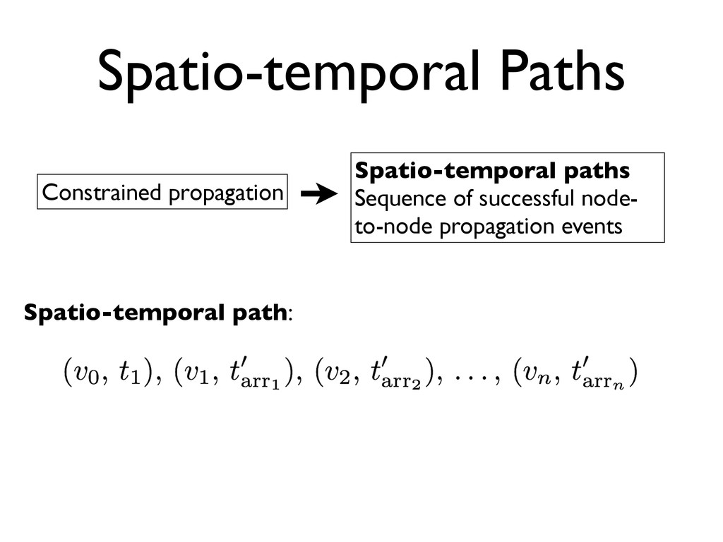
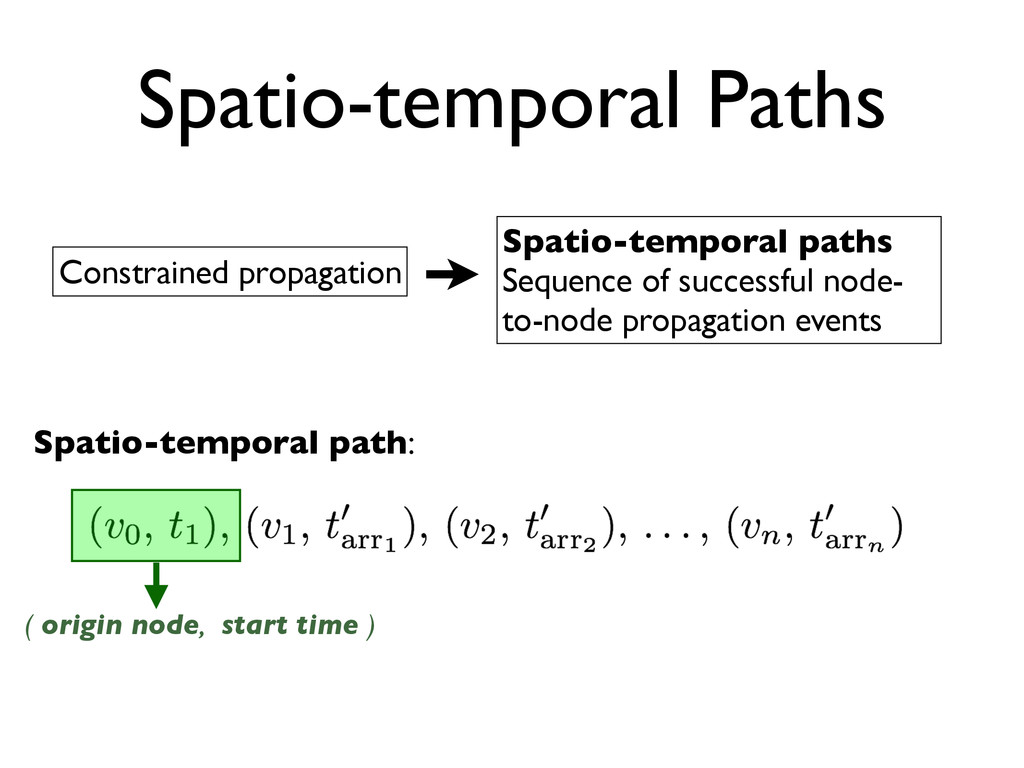
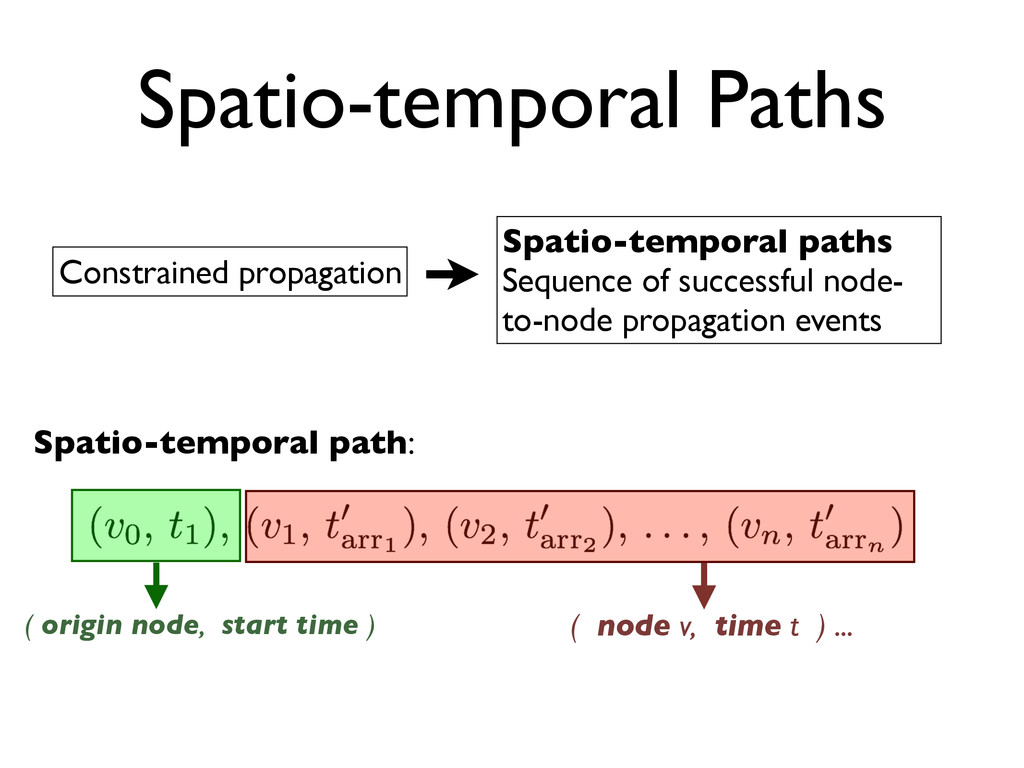
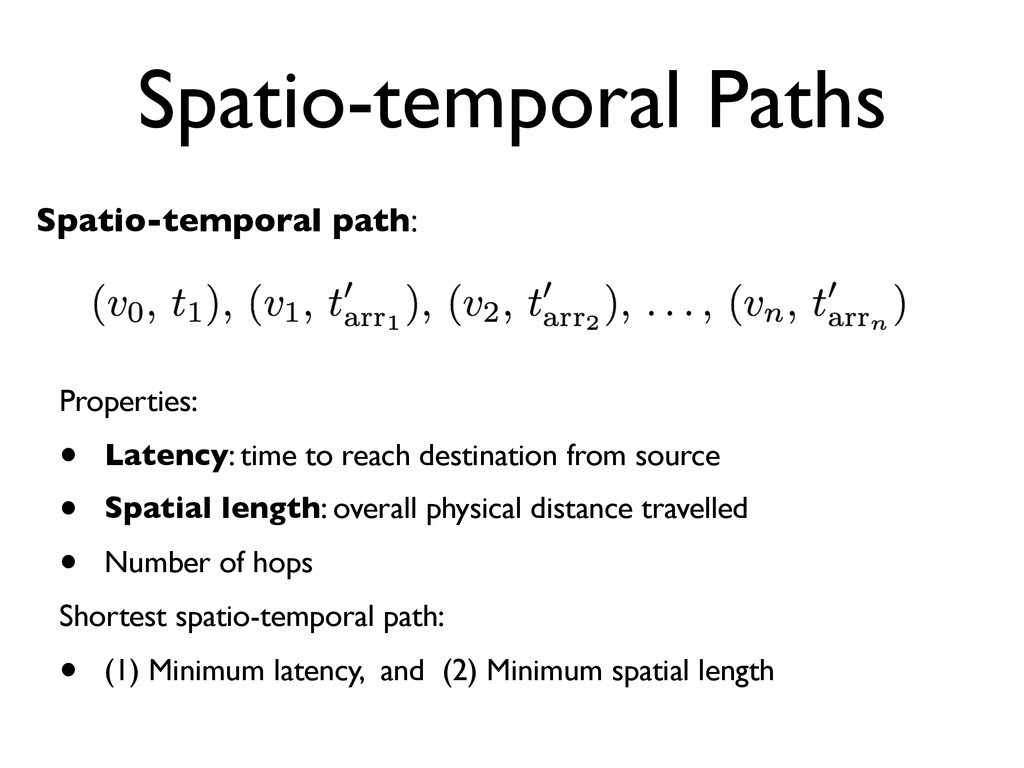
6. • Spatial: Nodes and edges embedded in space • Mobile: Nodes may be mobile (time-varying location) • Temporal: Time-evolving topology • Non-instantaneous interaction: Node-to-node interactions are constrained by space and may be non-instantaneous Generalised Spatio-Temporal Networks
7. London Underground (Metro Rapid Transit System) US Domestic Flights Example: Public Transport Process over the network = Passenger transit
8. Representation of spatio- temporal networks
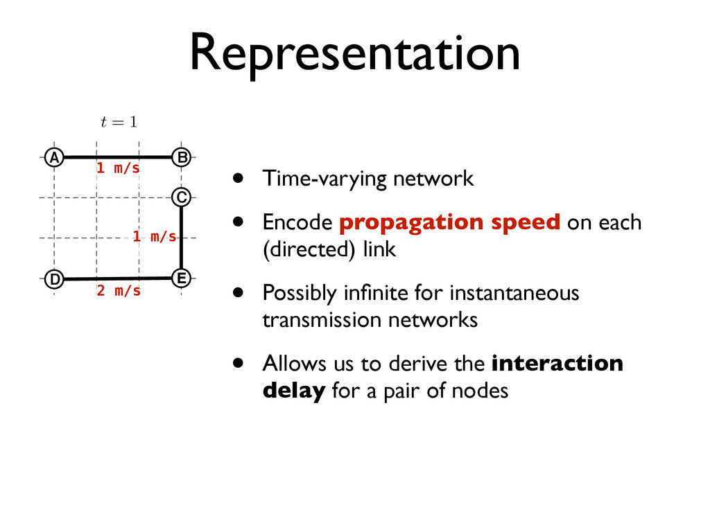
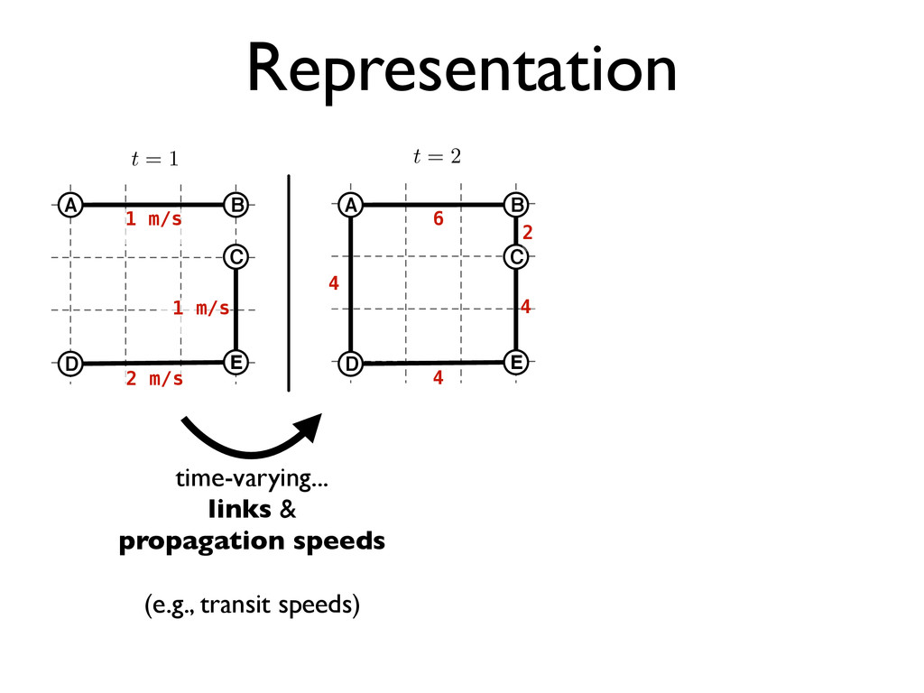
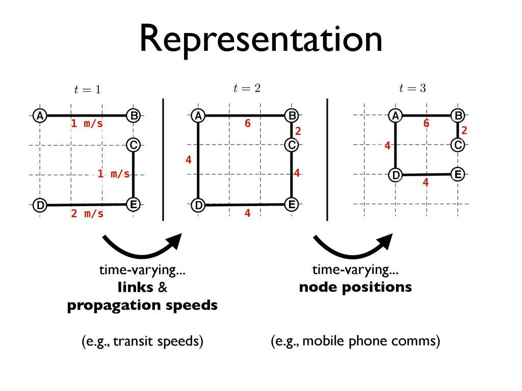
9. Representation t = 2 t = 1 t = 3 B C E D A B C E D A B C E D A 2 m/s 1 m/s 4 6 6 4 1 m/s 4 4 2 2 • Time-varying network • Encode propagation speed on each (directed) link • Possibly infinite for instantaneous transmission networks • Allows us to derive the interaction delay for a pair of nodes
10. t = 2 t = 1 t = 3 4 B C E D A B C E D A B C E D A 2 m/s 1 m/s 4 6 6 4 1 m/s 4 4 2 2 Representation time-varying... links & propagation speeds (e.g., transit speeds)
11. Representation time-varying... links & propagation speeds (e.g., transit speeds) time-varying... node positions (e.g., mobile phone comms) t = 2 t = 1 t = 3 4 B C E D A B C E D A B C E D A 2 m/s 1 m/s 4 6 6 4 1 m/s 4 4 2 2
12. Defining paths over spatio- temporal networks
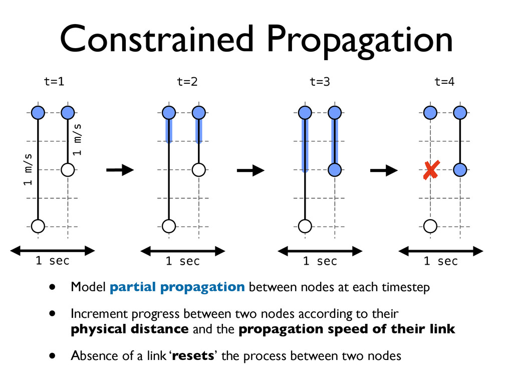
13. Constrained Propagation • Model partial propagation between nodes at each timestep • Increment progress between two nodes according to their physical distance and the propagation speed of their link • Absence of a link ‘resets’ the process between two nodes 1 m/s 1 m/s ✘ t=1 t=2 t=3 t=4 1 sec 1 sec 1 sec 1 sec
14. Spatio-temporal Paths Constrained propagation Spatio-temporal path: Spatio-temporal paths Sequence of successful node- to-node propagation events
15. Spatio-temporal Paths Constrained propagation Spatio-temporal path: Spatio-temporal paths Sequence of successful node- to-node propagation events ( origin node, start time )
16. Spatio-temporal Paths Constrained propagation Spatio-temporal path: Spatio-temporal paths Sequence of successful node- to-node propagation events ( origin node, start time ) ( node v, time t ) ...
17. Spatio-temporal Paths Constrained propagation Spatio-temporal path: Spatio-temporal paths Sequence of successful node- to-node propagation events like temporal paths, except... ( origin node, start time ) ( node v, time t ) ...
18. Spatio-temporal Paths Properties: • Latency: time to reach destination from source • Spatial length: overall physical distance travelled • Number of hops Shortest spatio-temporal path: • (1) Minimum latency, and (2) Minimum spatial length Spatio-temporal path:
19. Measuring robustness of spatio-temporal networks
20. Robustness of Spatio-Temporal Networks • How does the system respond to node failure? • The behaviour of a spatio-temporal network can be measured in terms of its topological, temporal, and spatial structure
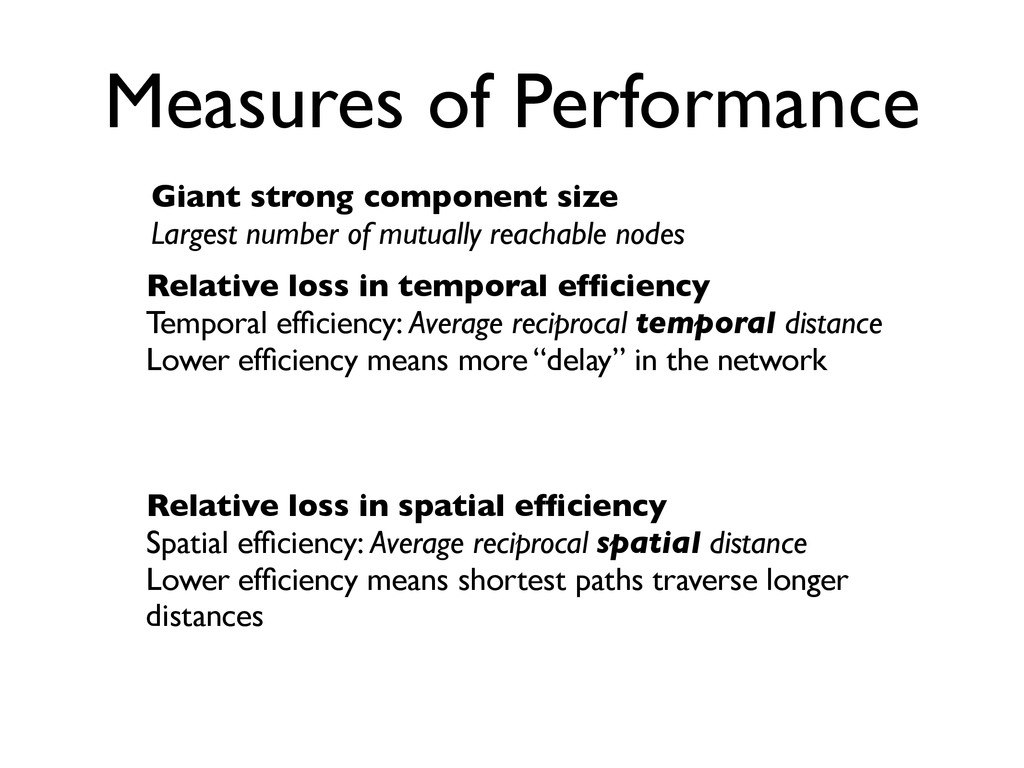
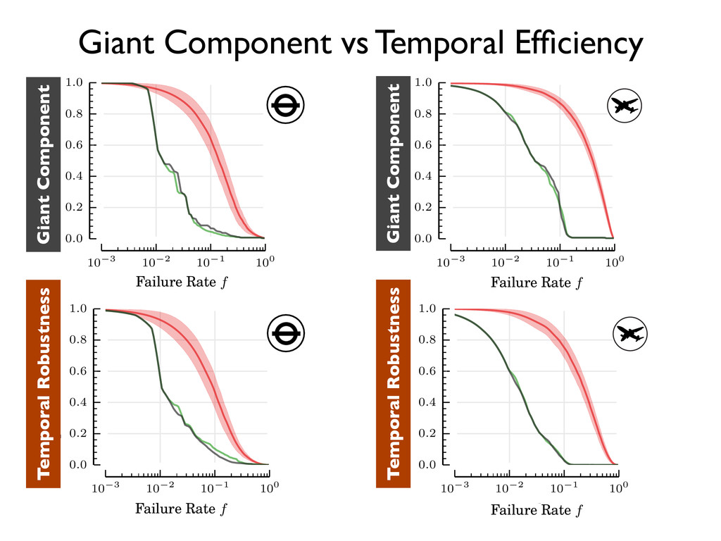
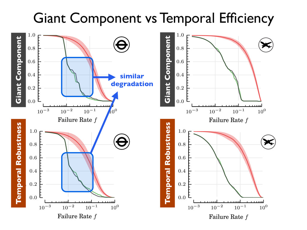
21. Measures of Performance Giant strong component size Largest number of mutually reachable nodes Relative loss in temporal efficiency Temporal efficiency: Average reciprocal temporal distance Lower efficiency means more “delay” in the network Relative loss in spatial efficiency Spatial efficiency: Average reciprocal spatial distance Lower efficiency means shortest paths traverse longer distances
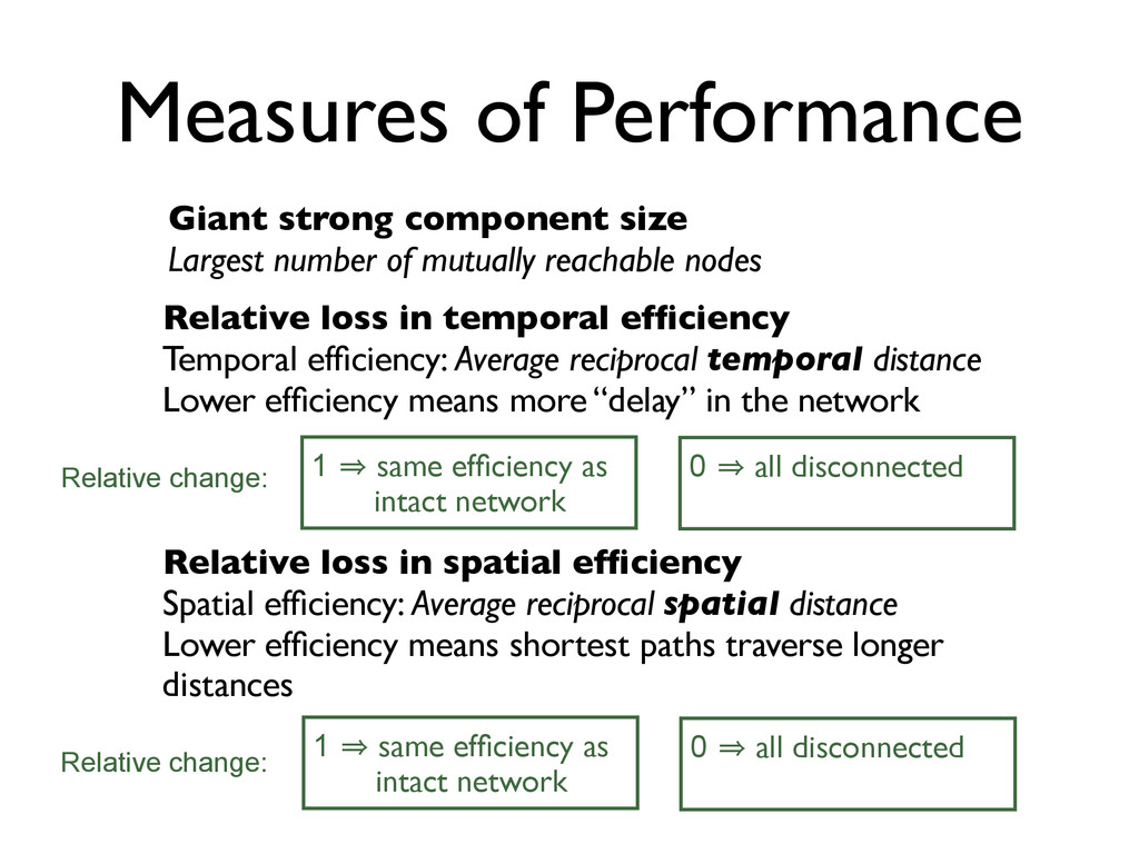
22. Measures of Performance Giant strong component size Largest number of mutually reachable nodes Relative loss in temporal efficiency Temporal efficiency: Average reciprocal temporal distance Lower efficiency means more “delay” in the network Relative loss in spatial efficiency Spatial efficiency: Average reciprocal spatial distance Lower efficiency means shortest paths traverse longer distances 1 㱺 same efficiency as intact network 0 㱺 all disconnected Relative change: 1 㱺 same efficiency as intact network 0 㱺 all disconnected Relative change:
23. Real-world Networks C. Elegans (Nematode) Neural Network (279 neurons) London Underground Passenger Transit (270 stations) US Domestic Flights Passenger Transit (299 Airports) StudentLife Mobile Comms (Calls & SMS Logs) (22 Dartmouth Students)
24. Propagation Type Nodes Edges (Aggregate Network) Time- Varying Topology Mobile Nodes Median Propagation Speed Underground Passenger Transit 270 628 ✔ ✘ 8 m/s Flights (U.S. Domestic) Passenger Transit 299 3947 ✔ ✘ 152 m/s C. Elegans (Neural Network) Synaptic Transmission 279 2990 ✘ ✘ 0.44 mm/s StudentLife (Mobile Comms) Phone Calls & SMS 22 68 ✔ ✔ instantaneous Real-world Networks
25. Node Failure: Random • Random failure • Node deactivated with failure probability f 10 3 10 2 10 1 100 Removal Rate f 0.0 0.1 0.2 0.3 0.4 0.5 0.6 0.7 Giant Component Size S Err PB TC ID OD BE Rand.
26. 0.0 0.2 0.4 0.6 0.8 1.0 Removal Rate f 0.0 0.2 0.4 0.6 0.8 1.0 Temporal Robustness R UNDERGROUND STUDENTLIFE FLIGHTS C. ELEGANS 0.0 0.2 0.4 0.6 0.8 1.0 Removal Rate f 0.0 0.2 0.4 0.6 0.8 1.0 Giant Component Size S UNDERGROUND STUDENTLIFE FLIGHTS C. ELEGANS 0.0 0.2 0.4 0.6 0.8 1.0 Removal Rate f 0.0 0.2 0.4 0.6 0.8 1.0 Spatial Robustness R& UNDERGROUND STUDENTLIFE FLIGHTS C. ELEGANS Resilience to Random Failure Temporal Reachability (Giant Temporal Comp.) Spatial ↘ ↓ → 0.0 0.2 0.4 0.6 0.8 1.0 Failure Rate f 0.0 0.2 0.4 0.6 0.8 1.0 Giant Component Size S UNDERGROUND STUDENTLIFE FLIGHTS C. ELEGANS 0.0 0.2 0.4 0.6 0.8 1.0 Failure Rate f 0.0 0.2 0.4 0.6 0.8 1.0 Giant Component Size S UNDERGROUND STUDENTLIFE FLIGHTS C. ELEGANS 0.0 0.2 0.4 0.6 0.8 1.0 Failure Rate f 0.0 0.2 0.4 0.6 0.8 1.0 Giant Component Size S UNDERGROUND STUDENTLIFE FLIGHTS C. ELEGANS
27. 0.0 0.2 0.4 0.6 0.8 1.0 Removal Rate f 0.0 0.2 0.4 0.6 0.8 1.0 Temporal Robustness R UNDERGROUND STUDENTLIFE FLIGHTS C. ELEGANS 0.0 0.2 0.4 0.6 0.8 1.0 Removal Rate f 0.0 0.2 0.4 0.6 0.8 1.0 Giant Component Size S UNDERGROUND STUDENTLIFE FLIGHTS C. ELEGANS 0.0 0.2 0.4 0.6 0.8 1.0 Removal Rate f 0.0 0.2 0.4 0.6 0.8 1.0 Spatial Robustness R& UNDERGROUND STUDENTLIFE FLIGHTS C. ELEGANS Resilience to Random Failure Temporal Reachability (Giant Temporal Comp.) Spatial ↘ ↓ → Underground highly fragile 0.0 0.2 0.4 0.6 0.8 1.0 Failure Rate f 0.0 0.2 0.4 0.6 0.8 1.0 Giant Component Size S UNDERGROUND STUDENTLIFE FLIGHTS C. ELEGANS 0.0 0.2 0.4 0.6 0.8 1.0 Failure Rate f 0.0 0.2 0.4 0.6 0.8 1.0 Giant Component Size S UNDERGROUND STUDENTLIFE FLIGHTS C. ELEGANS 0.0 0.2 0.4 0.6 0.8 1.0 Failure Rate f 0.0 0.2 0.4 0.6 0.8 1.0 Giant Component Size S UNDERGROUND STUDENTLIFE FLIGHTS C. ELEGANS
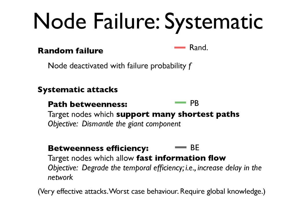
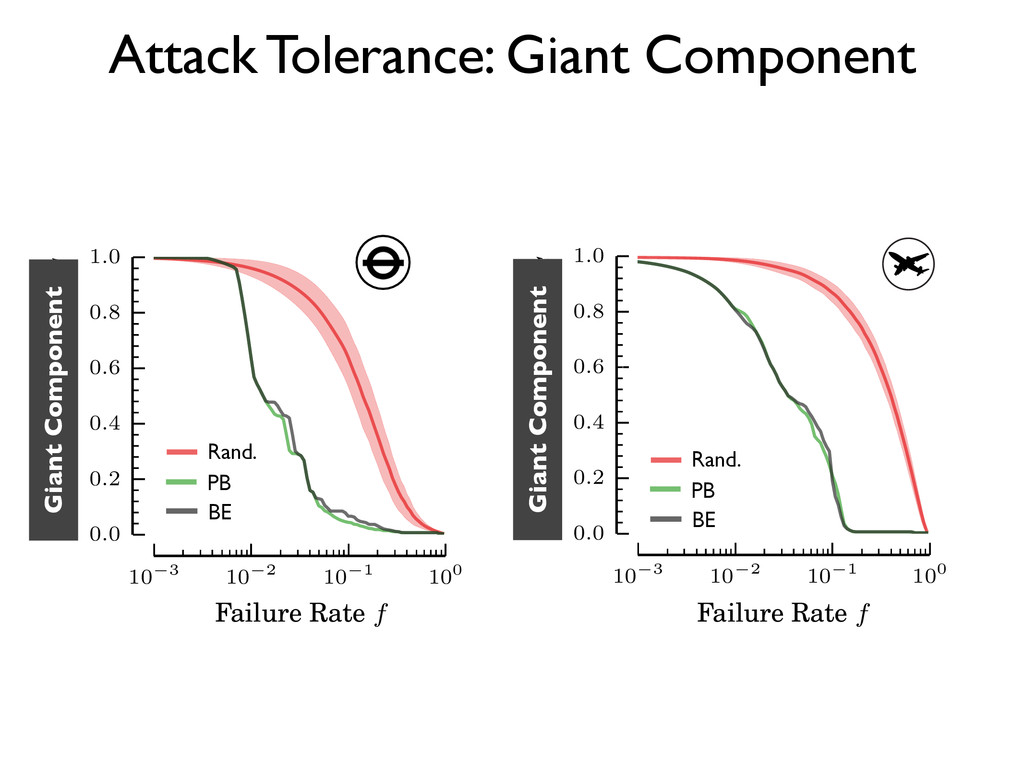
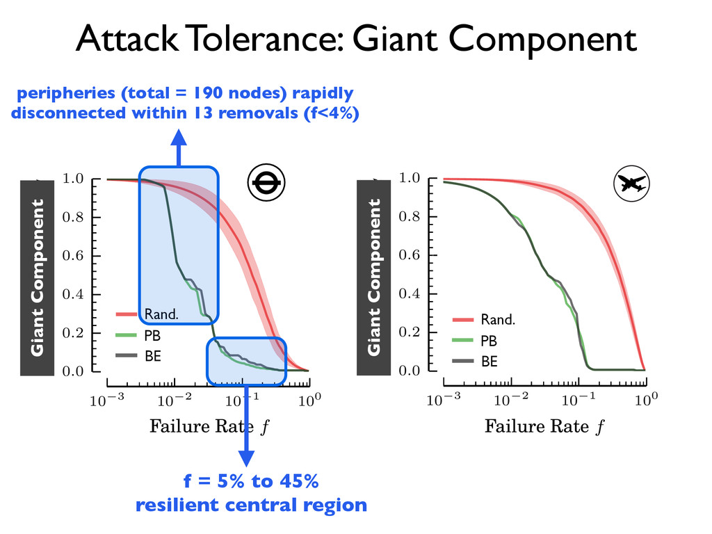
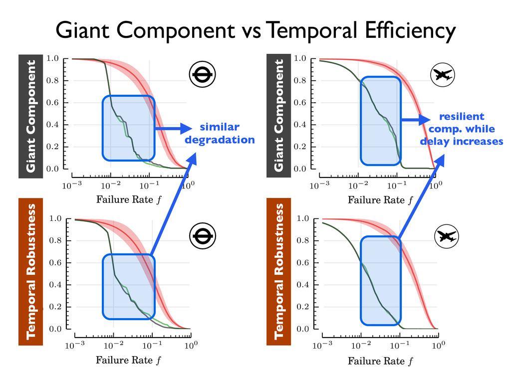
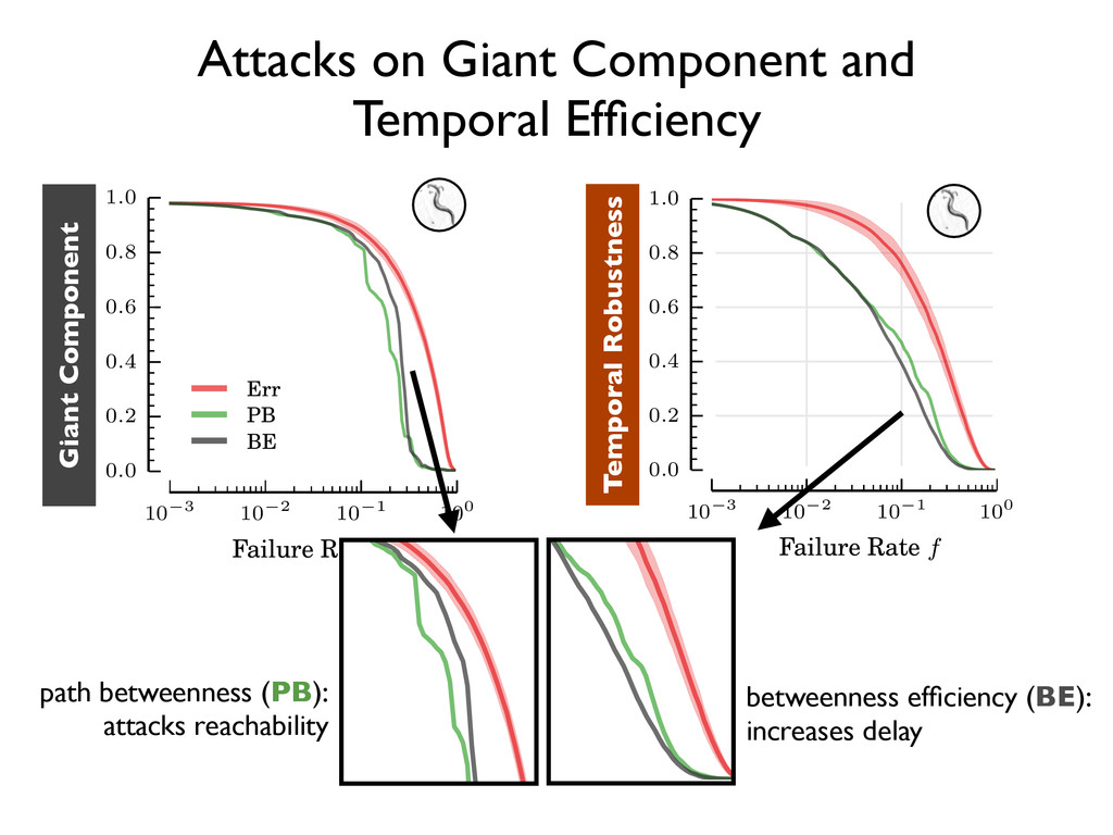
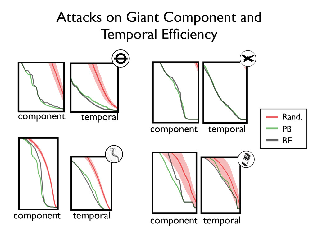
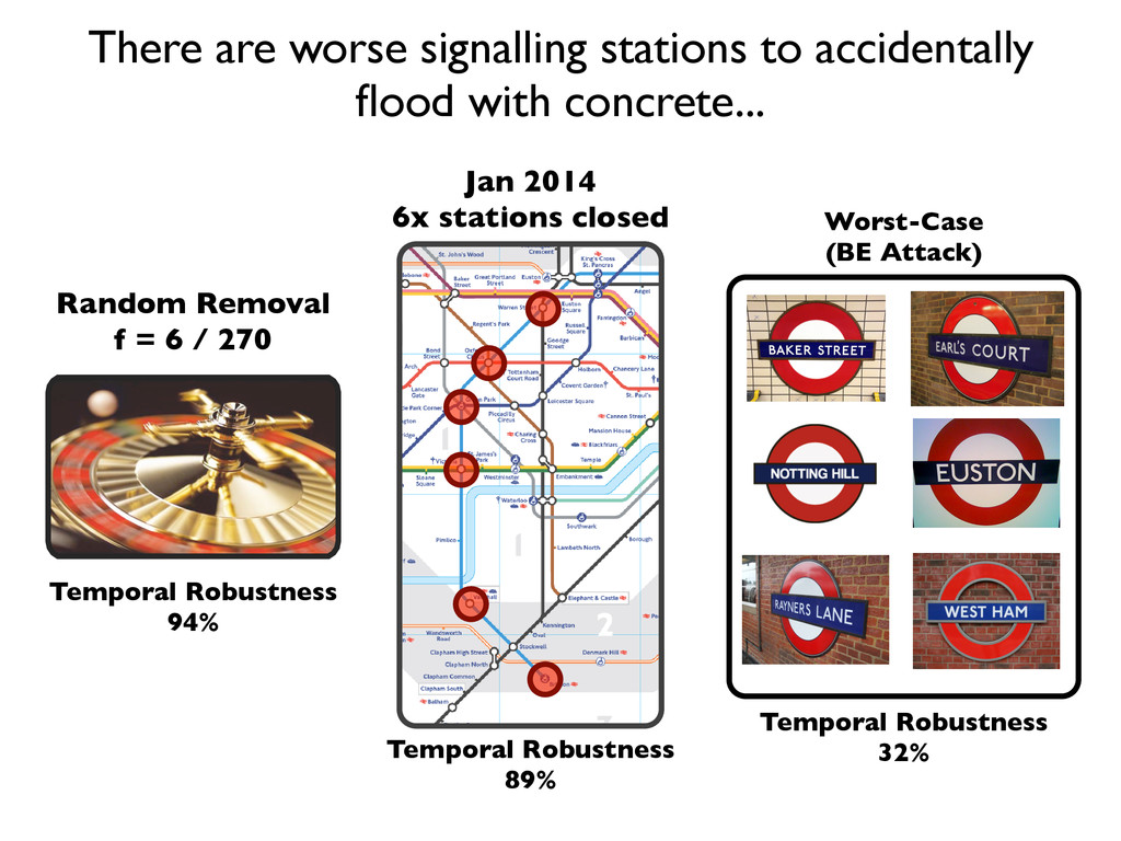
28. 10 3 10 2 10 1 100 Removal Rate f 0.0 0.1 0.2 0.3 0.4 0.5 0.6 0.7 Giant Component Size S Err PB TC ID OD BE PB Node Failure: Systematic • Random failure • Node deactivated with failure probability f • Systematic attacks • Path betweenness: Target nodes which support many shortest paths Objective: Dismantle the giant component • Betweenness efficiency: Target nodes which allow fast information flow Objective: Degrade the temporal efficiency; i.e., increase delay in the network • (Very effective attacks. Worst case behaviour. Require global knowledge.) 10 3 10 2 10 1 100 Removal Rate f 0.0 0.1 0.2 0.3 0.4 0.5 0.6 0.7 Giant Component Size S Err PB TC ID OD BE Rand. 10 3 10 2 10 1 100 Removal Rate f 0.0 0.1 0.2 0.3 0.4 0.5 0.6 0.7 Giant Component Size S Err PB TC ID OD BE BE
29. 10 3 10 2 10 1 100 Removal Rate f 0.0 0.2 0.4 0.6 0.8 1.0 Giant Component Size S Err PB BE 10 3 10 2 10 1 100 Removal Rate f 0.0 0.2 0.4 0.6 0.8 1.0 Giant Component Size S Err PB BE 0.0 0.2 0.4 0.6 0.8 1.0 Failure Rate f 0.0 0.2 0.4 0.6 0.8 1.0 Giant Component Size S UNDERGROUND STUDENTLIFE FLIGHTS C. ELEGANS 0.0 0.2 0.4 0.6 0.8 1.0 Failure Rate f 0.0 0.2 0.4 0.6 0.8 1.0 Giant Component Size S UNDERGROUND STUDENTLIFE FLIGHTS C. ELEGANS Attack Tolerance: Giant Component 10 3 10 2 10 1 100 Removal Rate f 0.0 0.1 0.2 0.3 0.4 0.5 0.6 0.7 Giant Component Size S Err PB TC ID OD BE PB 10 3 10 2 10 1 100 Removal Rate f 0.0 0.1 0.2 0.3 0.4 0.5 0.6 0.7 Giant Component Size S Err PB TC ID OD BE BE 10 3 10 2 10 1 100 Removal Rate f 0.0 0.1 0.2 0.3 0.4 0.5 0.6 0.7 Giant Component Size S Err PB TC ID OD BE Rand. 10 3 10 2 10 1 100 Removal Rate f 0.0 0.1 0.2 0.3 0.4 0.5 0.6 0.7 Giant Component Size S Err PB TC ID OD BE PB 10 3 10 2 10 1 100 Removal Rate f 0.0 0.1 0.2 0.3 0.4 0.5 0.6 0.7 Giant Component Size S Err PB TC ID OD BE BE 10 3 10 2 10 1 100 Removal Rate f 0.0 0.1 0.2 0.3 0.4 0.5 0.6 0.7 Giant Component Size S Err PB TC ID OD BE Rand. Giant Component Giant Component
30. 10 3 10 2 10 1 100 Removal Rate f 0.0 0.2 0.4 0.6 0.8 1.0 Giant Component Size S Err PB BE 10 3 10 2 10 1 100 Removal Rate f 0.0 0.2 0.4 0.6 0.8 1.0 Giant Component Size S Err PB BE 0.0 0.2 0.4 0.6 0.8 1.0 Failure Rate f 0.0 0.2 0.4 0.6 0.8 1.0 Giant Component Size S UNDERGROUND STUDENTLIFE FLIGHTS C. ELEGANS 0.0 0.2 0.4 0.6 0.8 1.0 Failure Rate f 0.0 0.2 0.4 0.6 0.8 1.0 Giant Component Size S UNDERGROUND STUDENTLIFE FLIGHTS C. ELEGANS Attack Tolerance: Giant Component 10 3 10 2 10 1 100 Removal Rate f 0.0 0.1 0.2 0.3 0.4 0.5 0.6 0.7 Giant Component Size S Err PB TC ID OD BE PB 10 3 10 2 10 1 100 Removal Rate f 0.0 0.1 0.2 0.3 0.4 0.5 0.6 0.7 Giant Component Size S Err PB TC ID OD BE BE 10 3 10 2 10 1 100 Removal Rate f 0.0 0.1 0.2 0.3 0.4 0.5 0.6 0.7 Giant Component Size S Err PB TC ID OD BE Rand. 10 3 10 2 10 1 100 Removal Rate f 0.0 0.1 0.2 0.3 0.4 0.5 0.6 0.7 Giant Component Size S Err PB TC ID OD BE PB 10 3 10 2 10 1 100 Removal Rate f 0.0 0.1 0.2 0.3 0.4 0.5 0.6 0.7 Giant Component Size S Err PB TC ID OD BE BE 10 3 10 2 10 1 100 Removal Rate f 0.0 0.1 0.2 0.3 0.4 0.5 0.6 0.7 Giant Component Size S Err PB TC ID OD BE Rand. f = 5% to 45% resilient central region peripheries (total = 190 nodes) rapidly disconnected within 13 removals (f<4%) Giant Component Giant Component
31. 10 3 10 2 10 1 100 Removal Rate f 0.0 0.2 0.4 0.6 0.8 1.0 Giant Component Size S Err PB BE 10 3 10 2 10 1 100 Removal Rate f 0.0 0.2 0.4 0.6 0.8 1.0 Giant Component Size S Err PB BE 0.0 0.2 0.4 0.6 0.8 1.0 Failure Rate f 0.0 0.2 0.4 0.6 0.8 1.0 Giant Component Size S UNDERGROUND STUDENTLIFE FLIGHTS C. ELEGANS 0.0 0.2 0.4 0.6 0.8 1.0 Failure Rate f 0.0 0.2 0.4 0.6 0.8 1.0 Giant Component Size S UNDERGROUND STUDENTLIFE FLIGHTS C. ELEGANS Attack Tolerance: Giant Component f = 16% 10 3 10 2 10 1 100 Removal Rate f 0.0 0.1 0.2 0.3 0.4 0.5 0.6 0.7 Giant Component Size S Err PB TC ID OD BE PB 10 3 10 2 10 1 100 Removal Rate f 0.0 0.1 0.2 0.3 0.4 0.5 0.6 0.7 Giant Component Size S Err PB TC ID OD BE BE 10 3 10 2 10 1 100 Removal Rate f 0.0 0.1 0.2 0.3 0.4 0.5 0.6 0.7 Giant Component Size S Err PB TC ID OD BE Rand. 10 3 10 2 10 1 100 Removal Rate f 0.0 0.1 0.2 0.3 0.4 0.5 0.6 0.7 Giant Component Size S Err PB TC ID OD BE PB 10 3 10 2 10 1 100 Removal Rate f 0.0 0.1 0.2 0.3 0.4 0.5 0.6 0.7 Giant Component Size S Err PB TC ID OD BE BE 10 3 10 2 10 1 100 Removal Rate f 0.0 0.1 0.2 0.3 0.4 0.5 0.6 0.7 Giant Component Size S Err PB TC ID OD BE Rand. f = 5% to 45% resilient central region peripheries (total = 190 nodes) rapidly disconnected within 13 removals (f<4%) Giant Component Giant Component
32. 10 3 10 2 10 1 100 Removal Rate f 0.0 0.2 0.4 0.6 0.8 1.0 Temporal Robustness R 10 3 10 2 10 1 100 Removal Rate f 0.0 0.2 0.4 0.6 0.8 1.0 Giant Component Size S 10 3 10 2 10 1 100 Removal Rate f 0.0 0.2 0.4 0.6 0.8 1.0 Temporal Robustness R 10 3 10 2 10 1 100 Removal Rate f 0.0 0.2 0.4 0.6 0.8 1.0 Giant Component Size S 0.0 0.2 0.4 0.6 0.8 1.0 Failure Rate f 0.0 0.2 0.4 0.6 0.8 1.0 Giant Component Size S UNDERGROUND STUDENTLIFE FLIGHTS C. ELEGANS 0.0 0.2 0.4 0.6 0.8 1.0 Failure Rate f 0.0 0.2 0.4 0.6 0.8 1.0 Giant Component Size S UNDERGROUND STUDENTLIFE FLIGHTS C. ELEGANS 0.0 0.2 0.4 0.6 0.8 1.0 Failure Rate f 0.0 0.2 0.4 0.6 0.8 1.0 Giant Component Size S UNDERGROUND STUDENTLIFE FLIGHTS C. ELEGANS 0.0 0.2 0.4 0.6 0.8 1.0 Failure Rate f 0.0 0.2 0.4 0.6 0.8 1.0 Giant Component Size S UNDERGROUND STUDENTLIFE FLIGHTS C. ELEGANS Giant Component vs Temporal Efficiency Giant Component Temporal Robustness Giant Component Temporal Robustness
33. 10 3 10 2 10 1 100 Removal Rate f 0.0 0.2 0.4 0.6 0.8 1.0 Temporal Robustness R 10 3 10 2 10 1 100 Removal Rate f 0.0 0.2 0.4 0.6 0.8 1.0 Giant Component Size S 10 3 10 2 10 1 100 Removal Rate f 0.0 0.2 0.4 0.6 0.8 1.0 Temporal Robustness R 10 3 10 2 10 1 100 Removal Rate f 0.0 0.2 0.4 0.6 0.8 1.0 Giant Component Size S 0.0 0.2 0.4 0.6 0.8 1.0 Failure Rate f 0.0 0.2 0.4 0.6 0.8 1.0 Giant Component Size S UNDERGROUND STUDENTLIFE FLIGHTS C. ELEGANS 0.0 0.2 0.4 0.6 0.8 1.0 Failure Rate f 0.0 0.2 0.4 0.6 0.8 1.0 Giant Component Size S UNDERGROUND STUDENTLIFE FLIGHTS C. ELEGANS 0.0 0.2 0.4 0.6 0.8 1.0 Failure Rate f 0.0 0.2 0.4 0.6 0.8 1.0 Giant Component Size S UNDERGROUND STUDENTLIFE FLIGHTS C. ELEGANS 0.0 0.2 0.4 0.6 0.8 1.0 Failure Rate f 0.0 0.2 0.4 0.6 0.8 1.0 Giant Component Size S UNDERGROUND STUDENTLIFE FLIGHTS C. ELEGANS Giant Component vs Temporal Efficiency Giant Component Temporal Robustness Giant Component Temporal Robustness similar degradation
34. 10 3 10 2 10 1 100 Removal Rate f 0.0 0.2 0.4 0.6 0.8 1.0 Temporal Robustness R 10 3 10 2 10 1 100 Removal Rate f 0.0 0.2 0.4 0.6 0.8 1.0 Giant Component Size S 10 3 10 2 10 1 100 Removal Rate f 0.0 0.2 0.4 0.6 0.8 1.0 Temporal Robustness R 10 3 10 2 10 1 100 Removal Rate f 0.0 0.2 0.4 0.6 0.8 1.0 Giant Component Size S 0.0 0.2 0.4 0.6 0.8 1.0 Failure Rate f 0.0 0.2 0.4 0.6 0.8 1.0 Giant Component Size S UNDERGROUND STUDENTLIFE FLIGHTS C. ELEGANS 0.0 0.2 0.4 0.6 0.8 1.0 Failure Rate f 0.0 0.2 0.4 0.6 0.8 1.0 Giant Component Size S UNDERGROUND STUDENTLIFE FLIGHTS C. ELEGANS 0.0 0.2 0.4 0.6 0.8 1.0 Failure Rate f 0.0 0.2 0.4 0.6 0.8 1.0 Giant Component Size S UNDERGROUND STUDENTLIFE FLIGHTS C. ELEGANS 0.0 0.2 0.4 0.6 0.8 1.0 Failure Rate f 0.0 0.2 0.4 0.6 0.8 1.0 Giant Component Size S UNDERGROUND STUDENTLIFE FLIGHTS C. ELEGANS Giant Component vs Temporal Efficiency Giant Component Temporal Robustness Giant Component Temporal Robustness similar degradation resilient comp. while delay increases
35. 10 3 10 2 10 1 100 Removal Rate f 0.0 0.2 0.4 0.6 0.8 1.0 Temporal Robustness R 10 3 10 2 10 1 100 Removal Rate f 0.0 0.2 0.4 0.6 0.8 1.0 Giant Component Size S Err PB BE 0.0 0.2 0.4 0.6 0.8 1.0 Failure Rate f 0.0 0.2 0.4 0.6 0.8 1.0 Giant Component Size S UNDERGROUND STUDENTLIFE FLIGHTS C. ELEGANS 0.0 0.2 0.4 0.6 0.8 1.0 Failure Rate f 0.0 0.2 0.4 0.6 0.8 1.0 Giant Component Size S UNDERGROUND STUDENTLIFE FLIGHTS C. ELEGANS Attacks on Giant Component and Temporal Efficiency 0.0 10.0 20.0 30.0 40.0 50.0 60.0 Temporal Efficiency E ⇥10 3 Err PB BE 0.2 0.4 0.6 0.8 1.0 Err PB path betweenness (PB): attacks reachability betweenness efficiency (BE): increases delay Giant Component Temporal Robustness
36. 10 3 10 2 1 Removal R 0.0 0.1 0.2 0.3 0.4 0.5 0.6 0.7 Giant Component Size S Err PB TC ID OD BE PB 10 3 10 2 1 Removal R 0.0 0.1 0.2 0.3 0.4 0.5 0.6 0.7 Giant Component Size S Err PB TC ID OD BE BE 10 3 10 2 1 Removal R 0.0 0.1 0.2 0.3 0.4 0.5 0.6 0.7 Giant Component Size S Err PB TC ID OD BE Rand. Attacks on Giant Component and Temporal Efficiency 10 3 10 2 10 1 100 Removal Rate f 0.0 0.2 0.4 0.6 0.8 1.0 Giant Component Size S 10 3 10 2 10 1 100 Removal Rate f 0.0 5.0 10.0 15.0 20.0 25.0 30.0 35.0 40.0 Temporal Efficiency E ⇥10 3 component temporal 10 2 10 1 100 Removal Rate f 10 3 10 2 10 1 100 Removal Rate f 0.0 1.0 2.0 3.0 4.0 5.0 6.0 7.0 ⇥10 3 0 2 10 1 100 emoval Rate f 10 3 10 2 10 1 100 Removal Rate f 0.0 10.0 20.0 30.0 40.0 50.0 60.0 Temporal Efficiency E ⇥10 3 component temporal component temporal 10 3 10 2 10 1 100 0.0 0.1 0.2 0.3 0.4 0.5 0.6 0.7 Giant Component Size S 10 3 10 2 10 1 100 Removal Rate f 0.0 1.0 2.0 3.0 4.0 5.0 6.0 7.0 8.0 9.0 Temporal Efficiency E ⇥10 3 component temporal
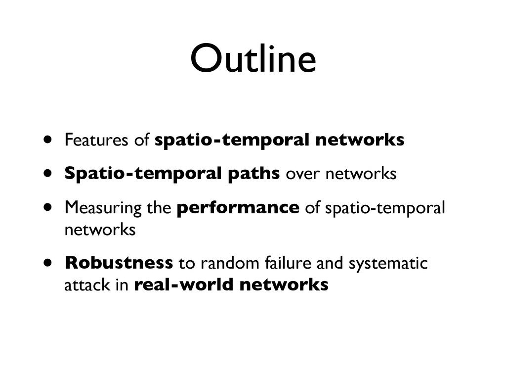
37. Summary I • Framework for modelling spatio-temporal systems as networks • Generalisation of temporal networks with spatially embedded nodes and paths that preserve space-time constraints • Avoids over-simplification due to aggregation (static network models) and instantaneous transmission (temporal network models)
38. Summary II • Systematic attacks can be designed to target different aspects of a network; e.g., topological (reachability) vs. temporal structure • Path betweenness attack – dismantles the giant component • Betweenness efficiency attack – increases delay
39. There are worse signalling stations to accidentally flood with concrete... Jan 2014 6x stations closed Temporal Robustness 89% Temporal Robustness 32% Worst-Case (BE Attack) Random Removal f = 6 / 270 Temporal Robustness 94%
40. Spatio-Temporal Complex Networks: Reachability, Centrality, and Robustness Matthew J. Williams University of Birmingham & University College London mattjw@mattjw.net http://www.mattjw.net @voxmjw Mirco Musolesi University College London Thanks for listening! http://arxiv.org/abs/1506.00627 @mircomusolesi
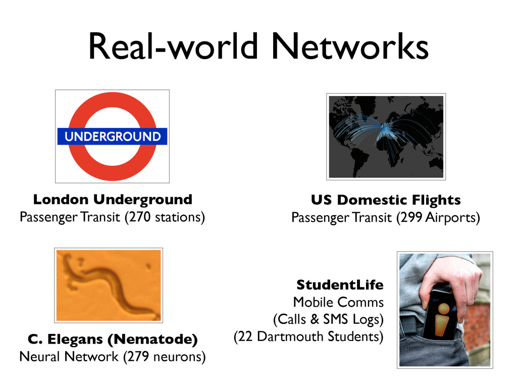
41. Attribution Globe “Earth - Illustration”. DonkeyHotey (Flickr CC). May 2011. https://www.flickr.com/photos/donkeyhotey/5679642871 C. Elegans “I: these are nematodes”. snickclunk (Flickr CC). July 2006. https://www.flickr.com/photos/snickclunk/200926410 Roulette Wheel “roulette”. eatsmilesleep (Flickr CC). August 2011. https://www.flickr.com/photos/45378259@N05/6050121954