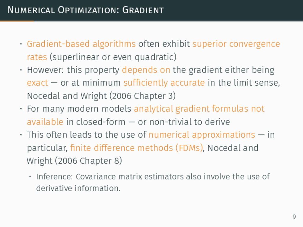
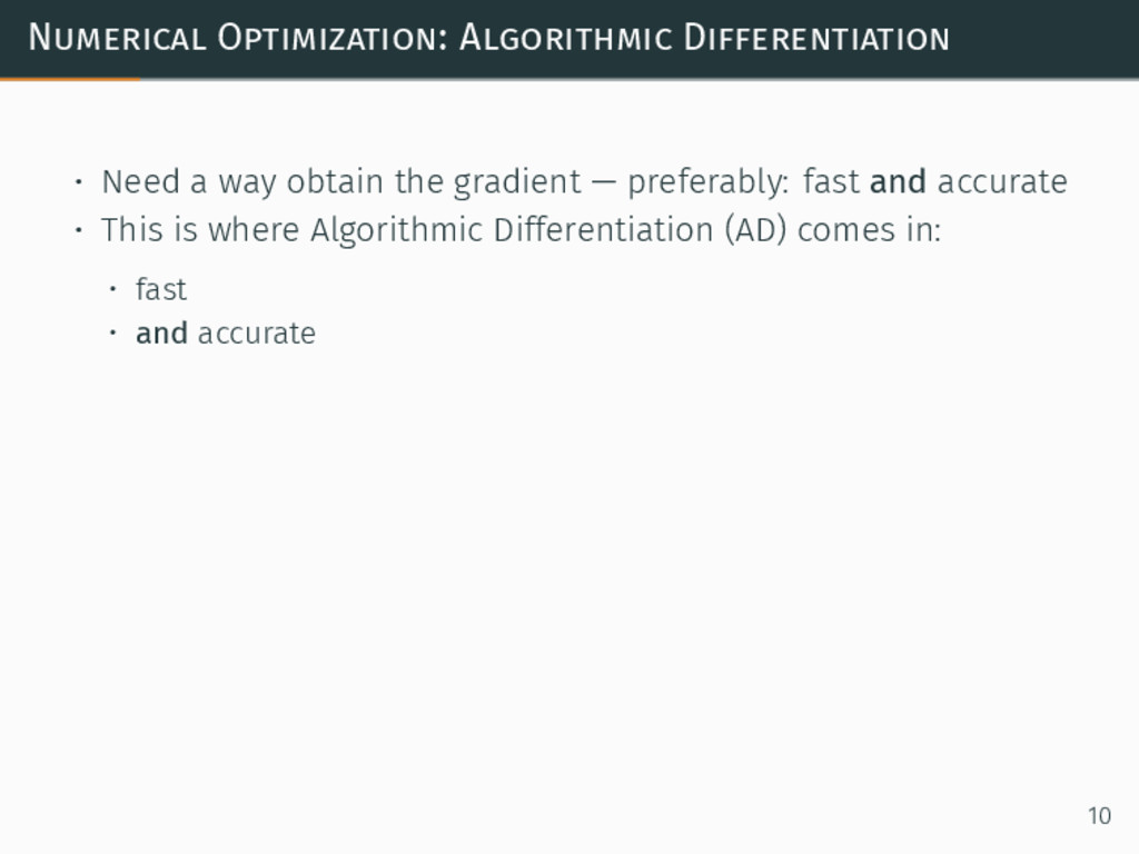
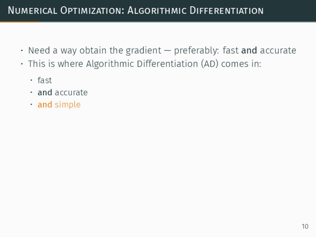
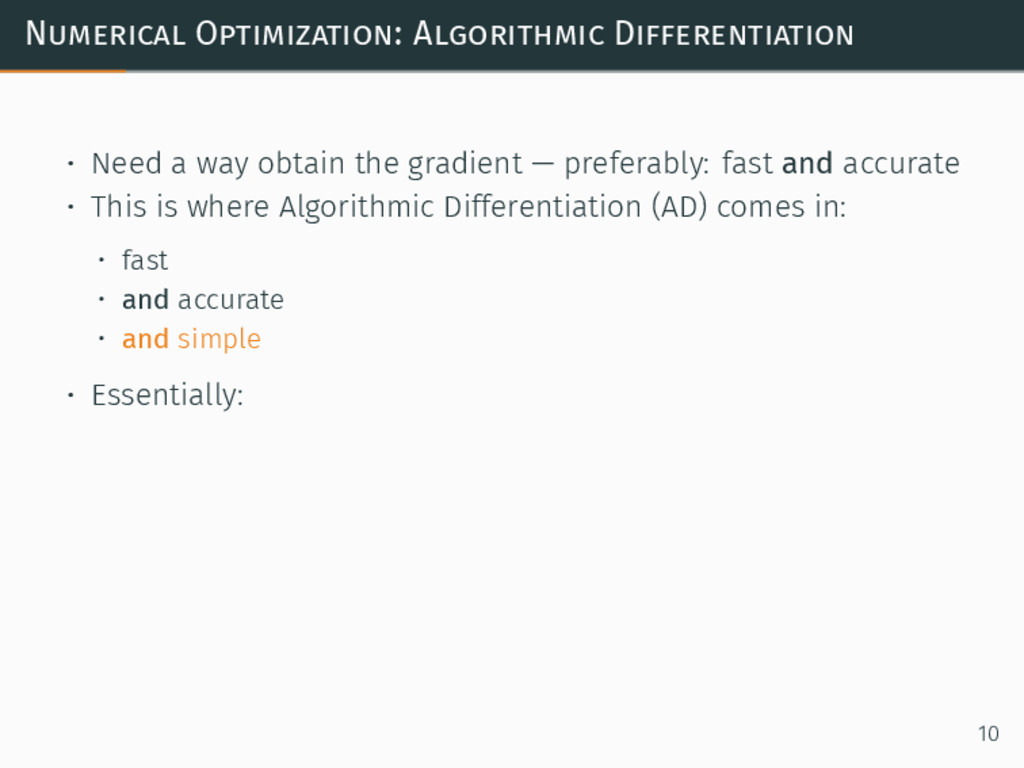
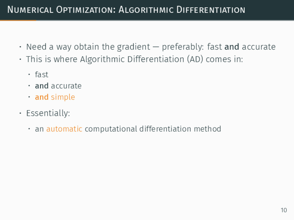
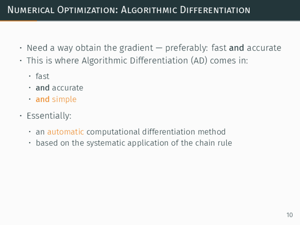
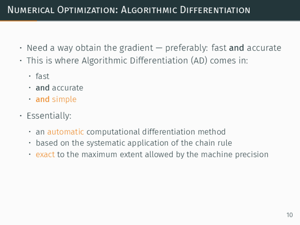
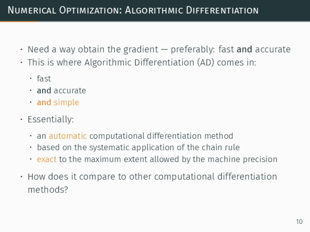
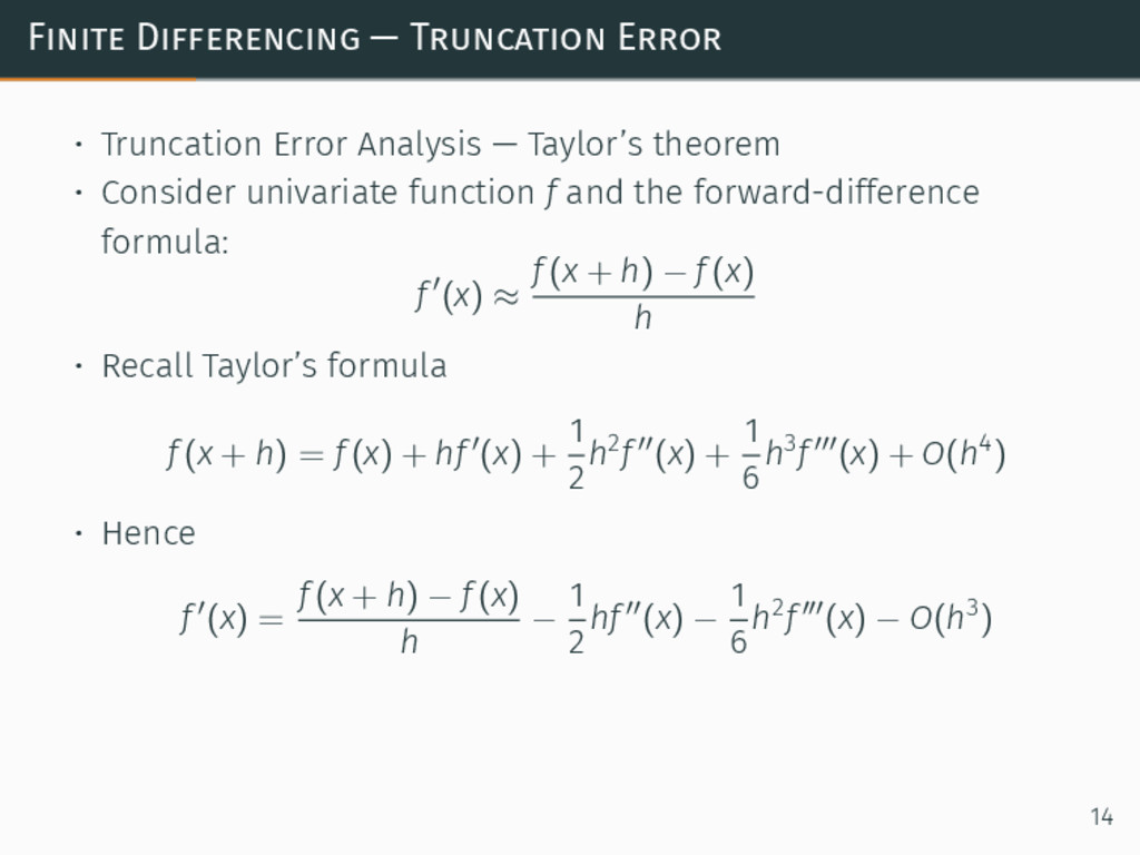
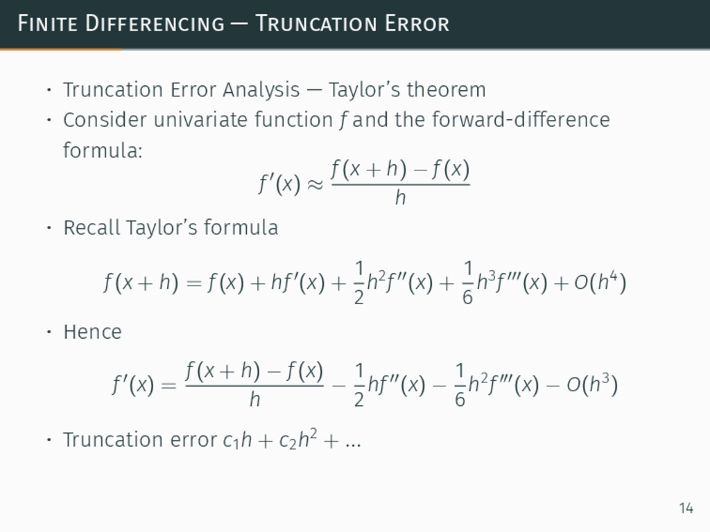
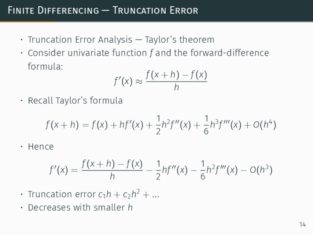
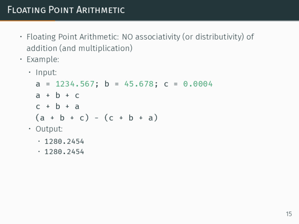
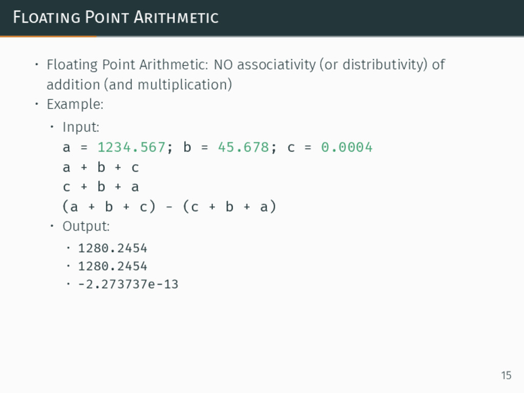
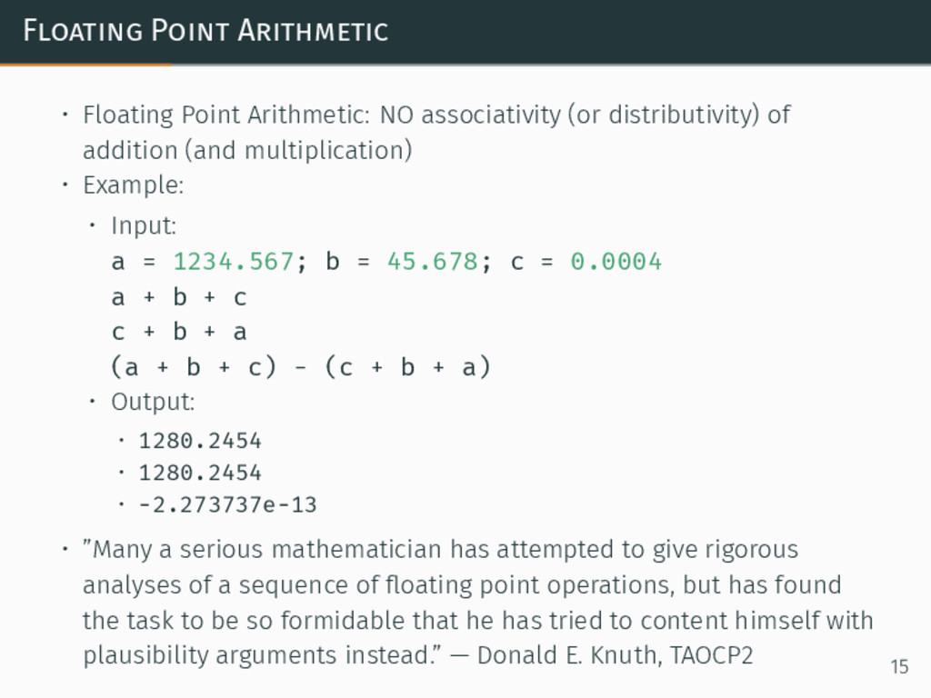
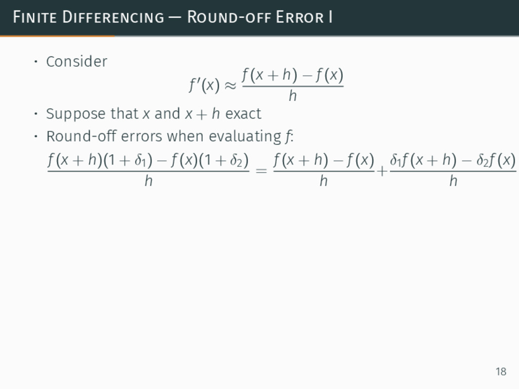
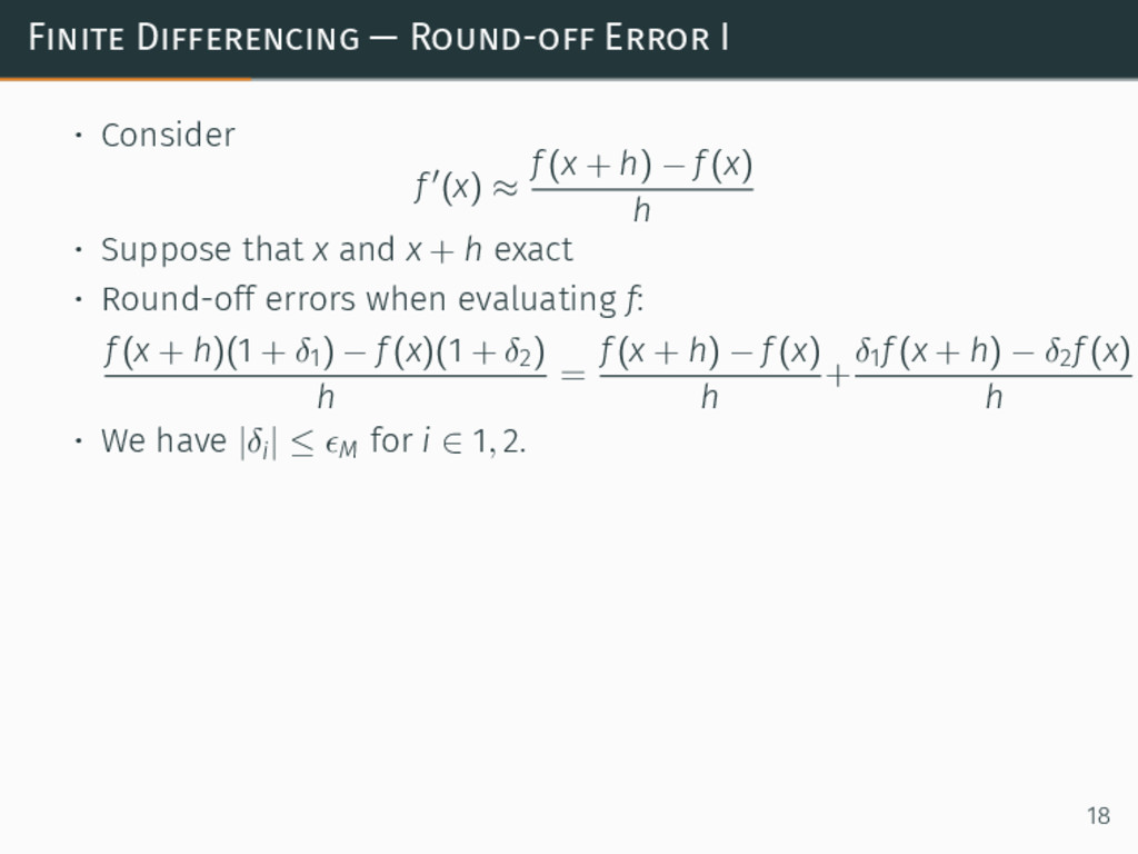
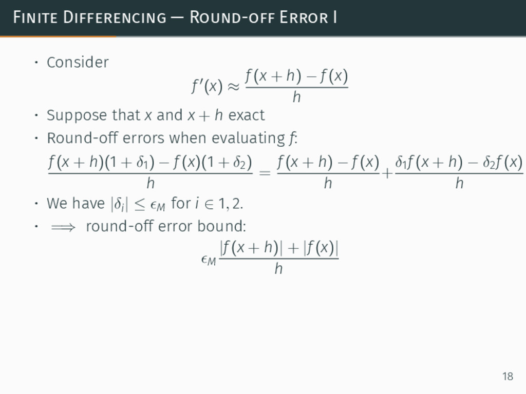
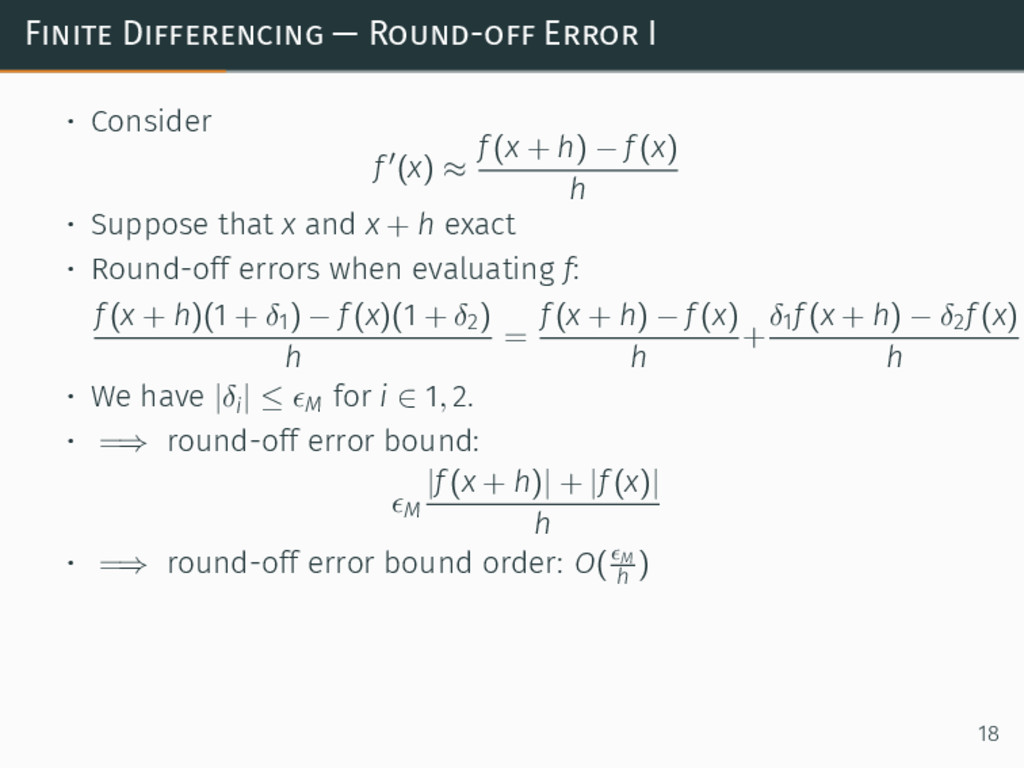
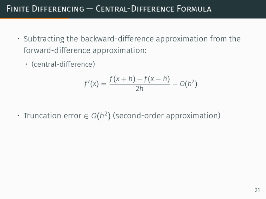
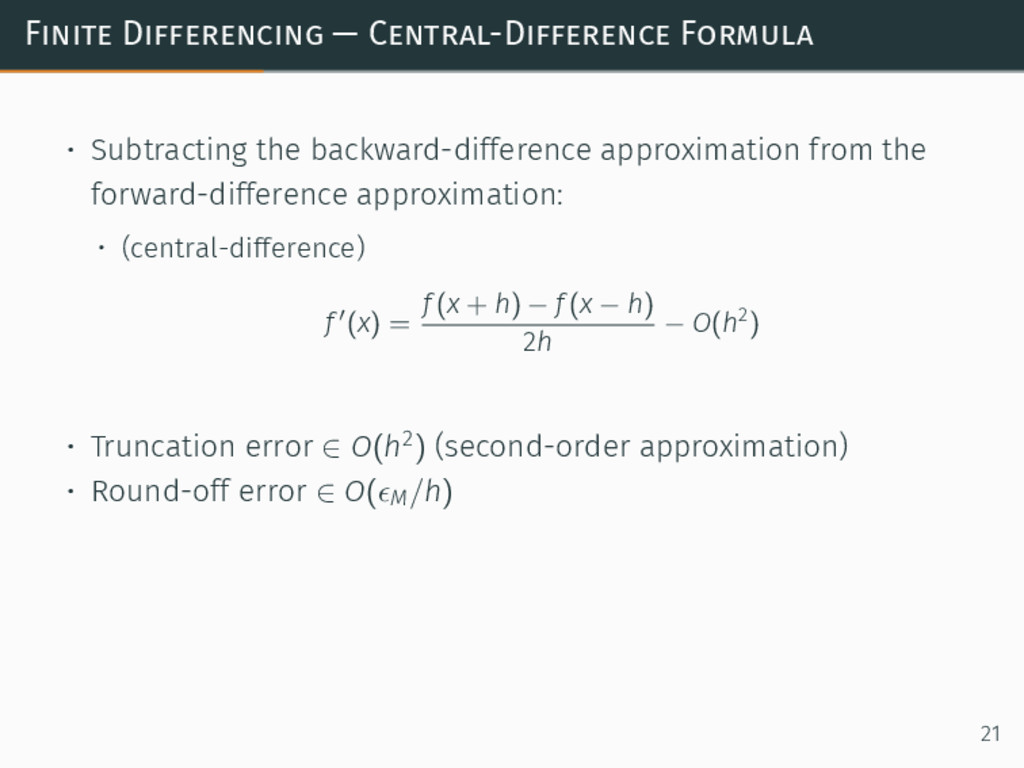
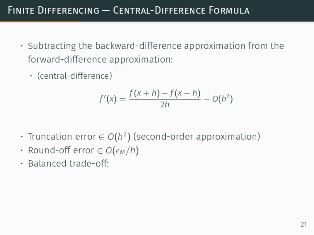
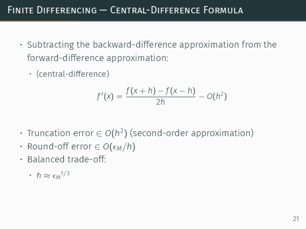
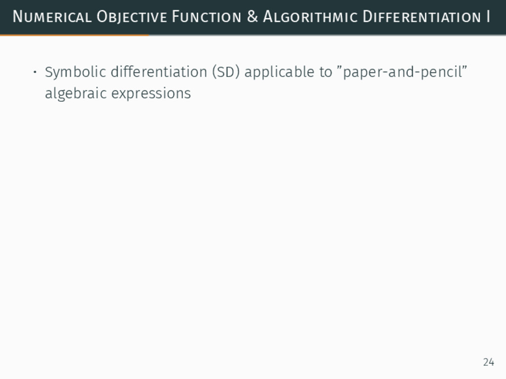
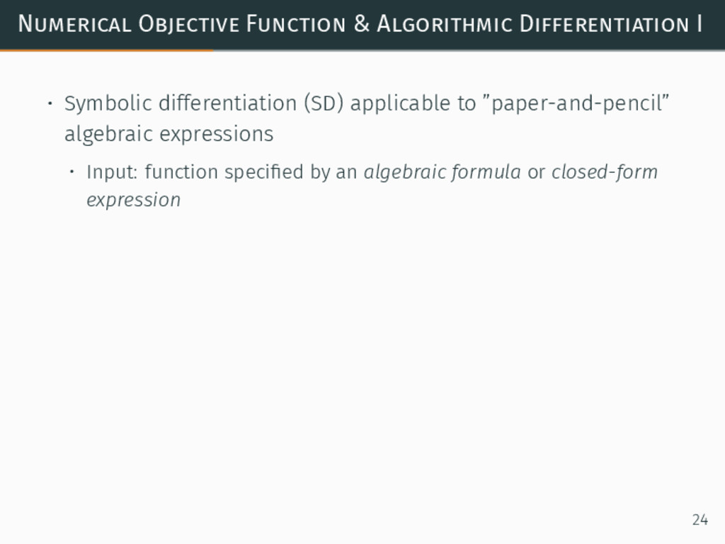
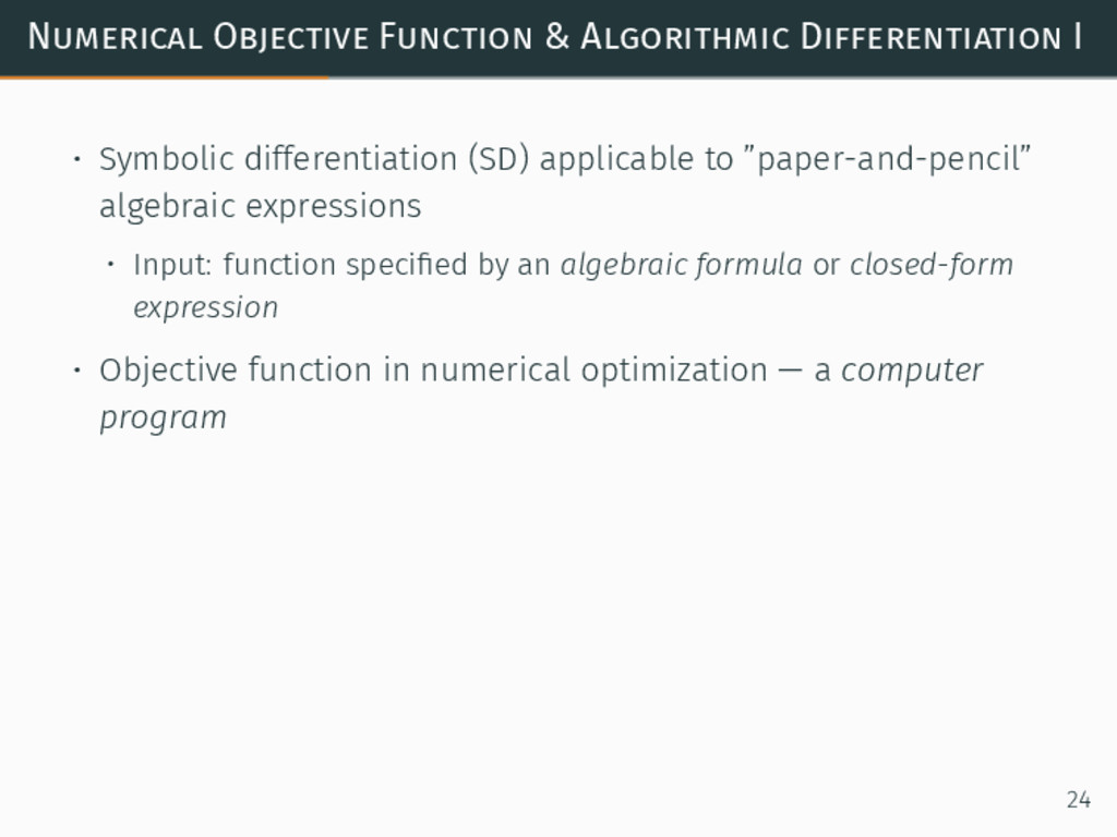
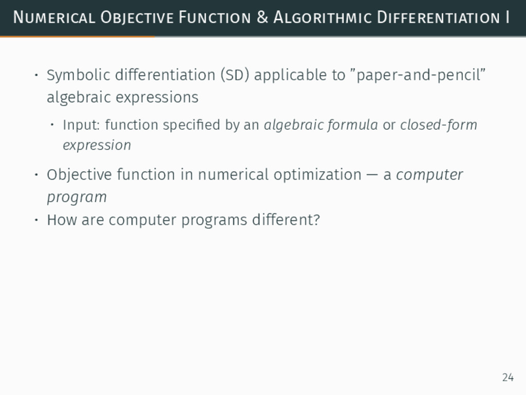
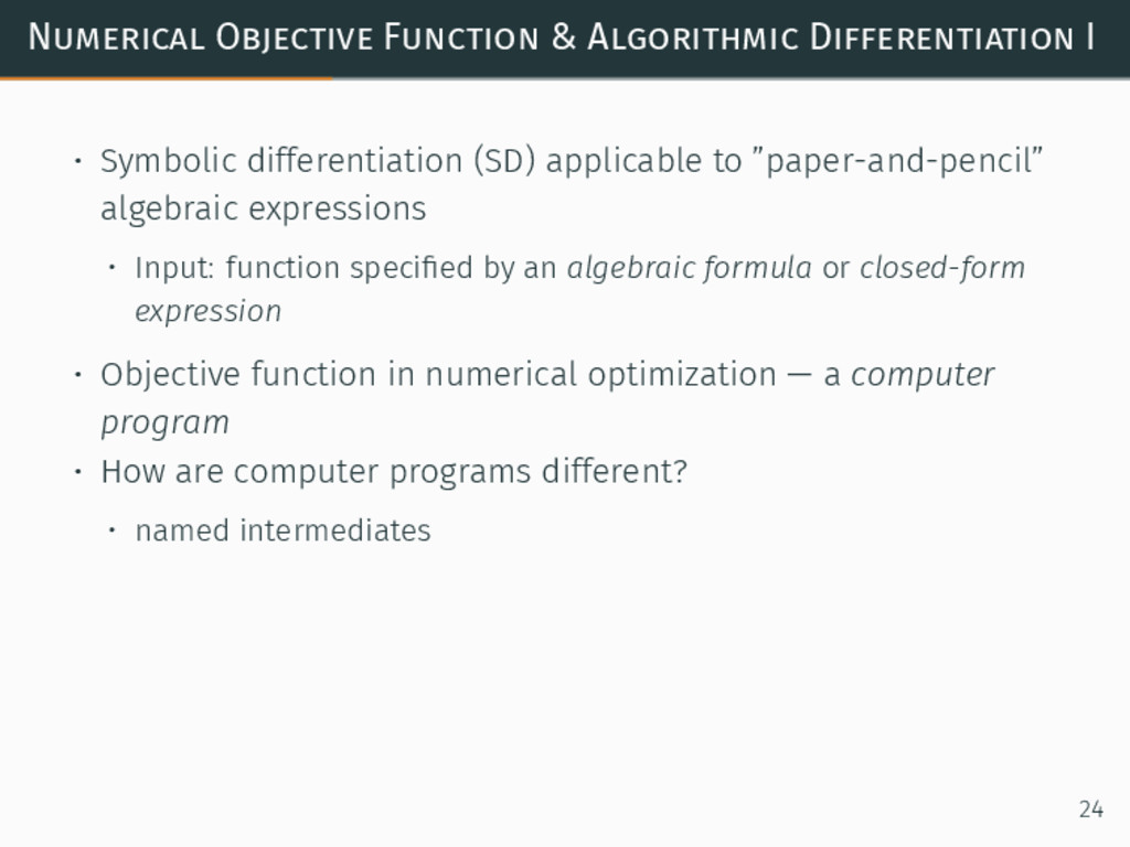
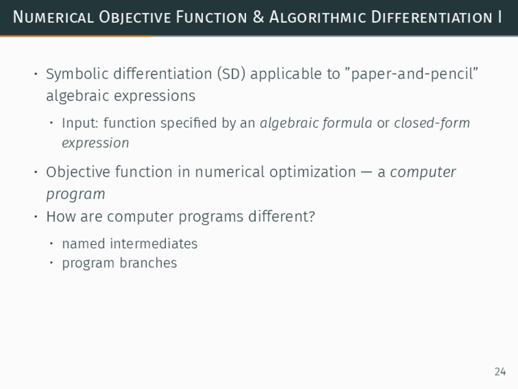
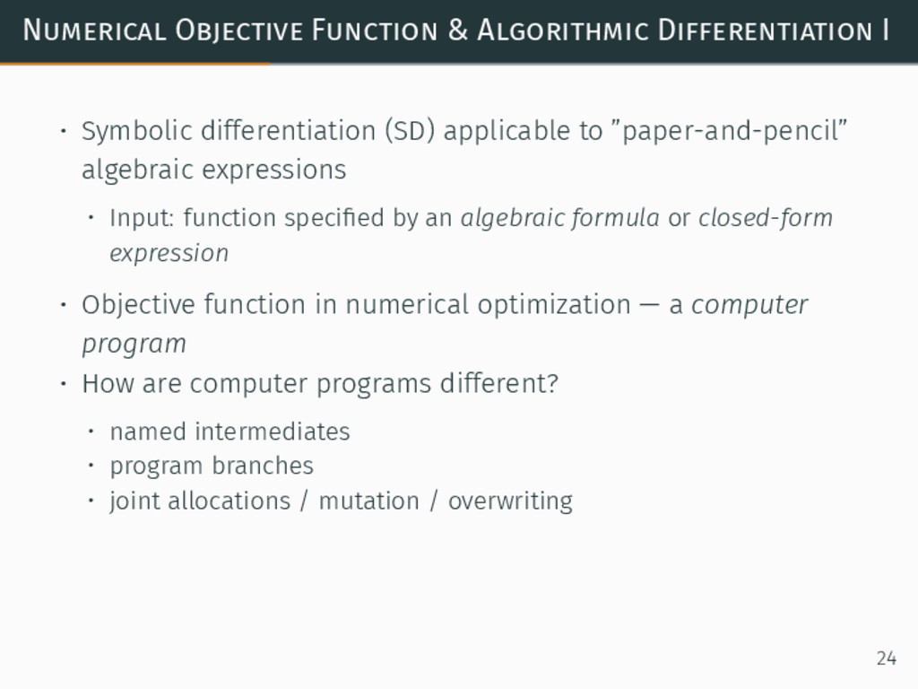
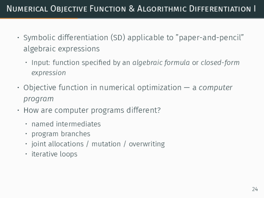
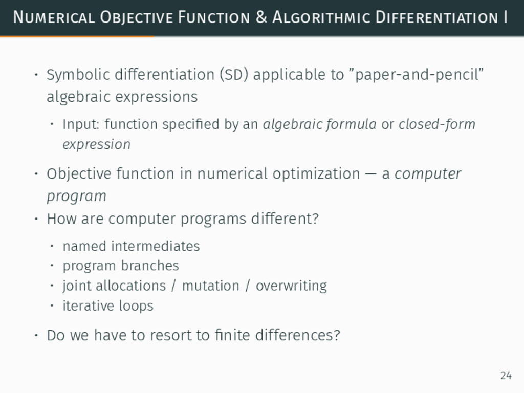
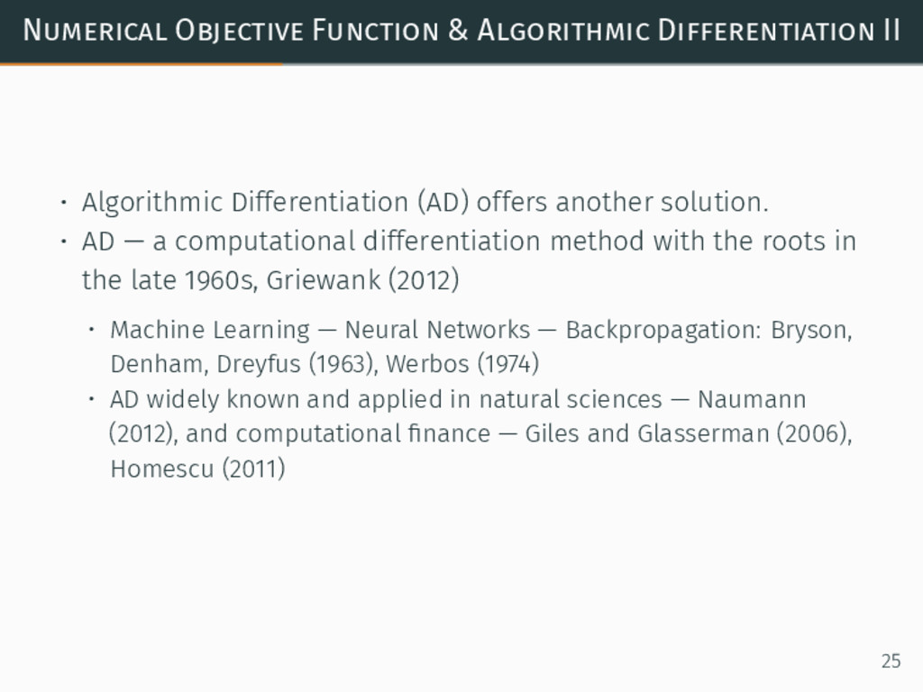
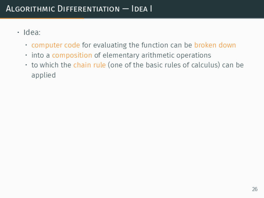
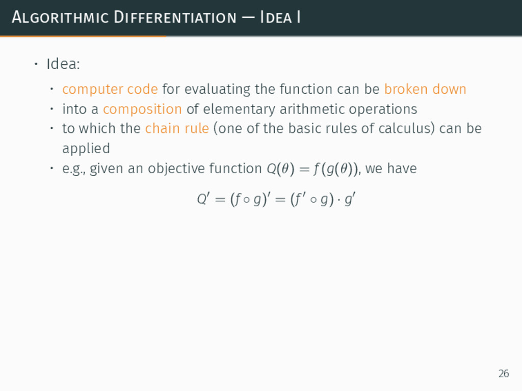
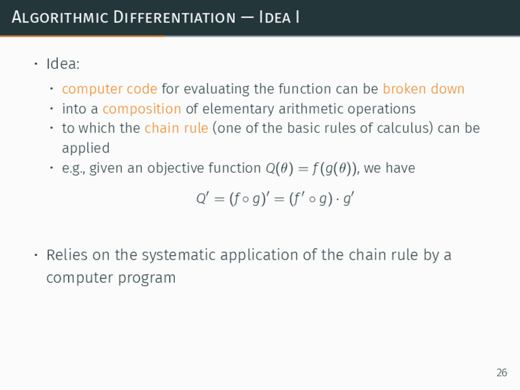
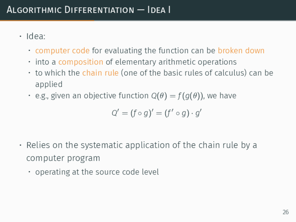
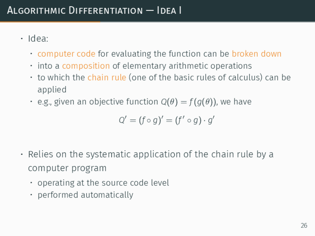
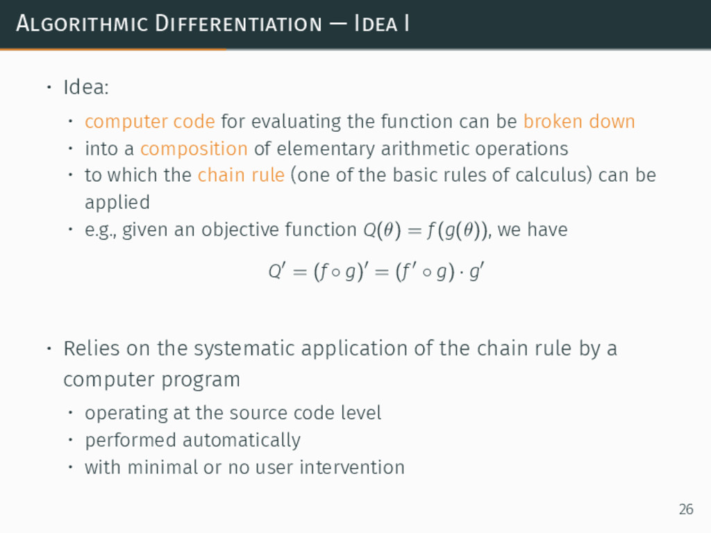
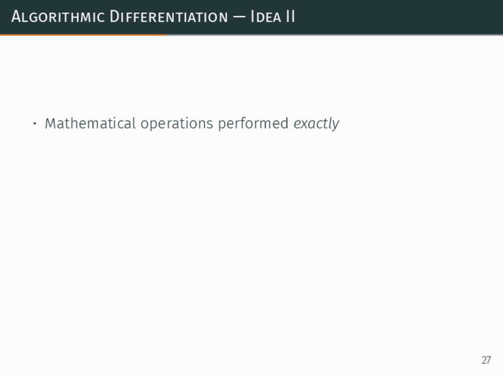
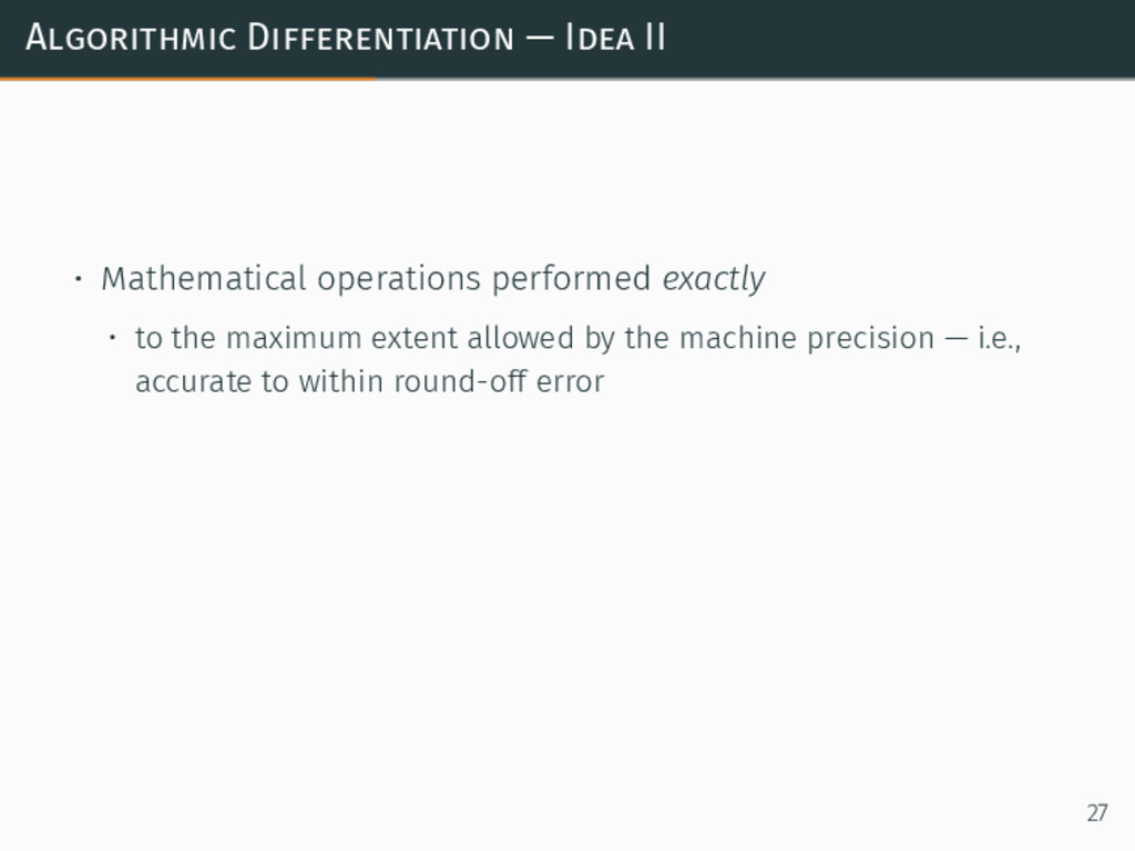
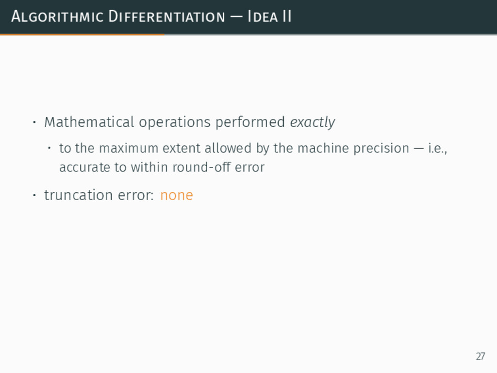
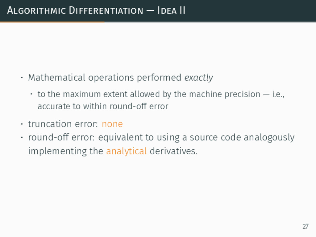
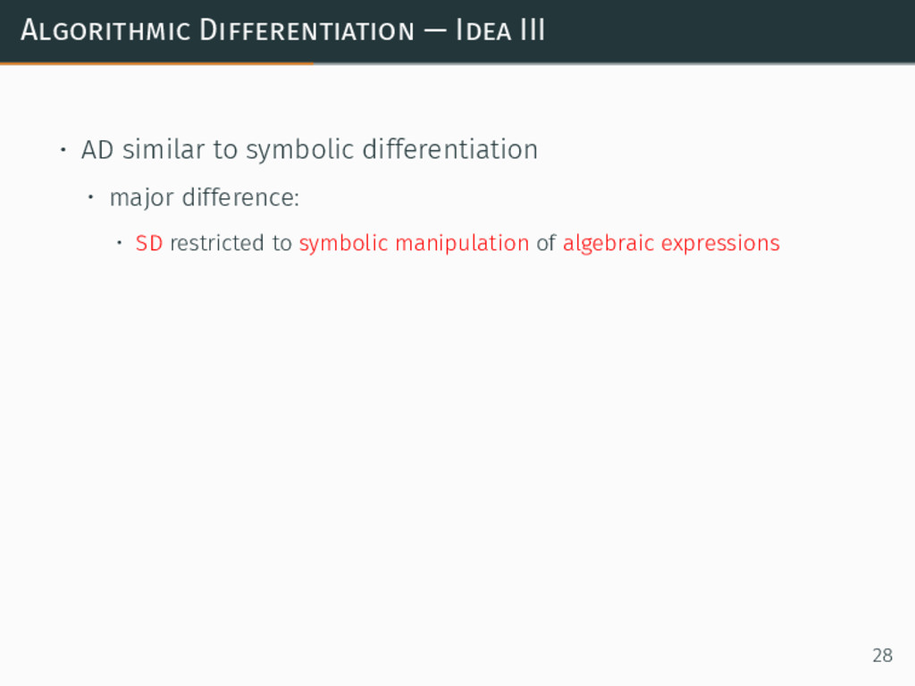
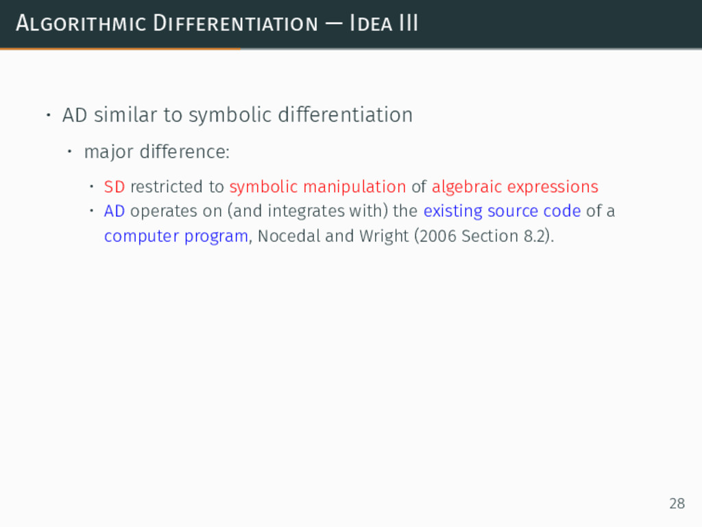
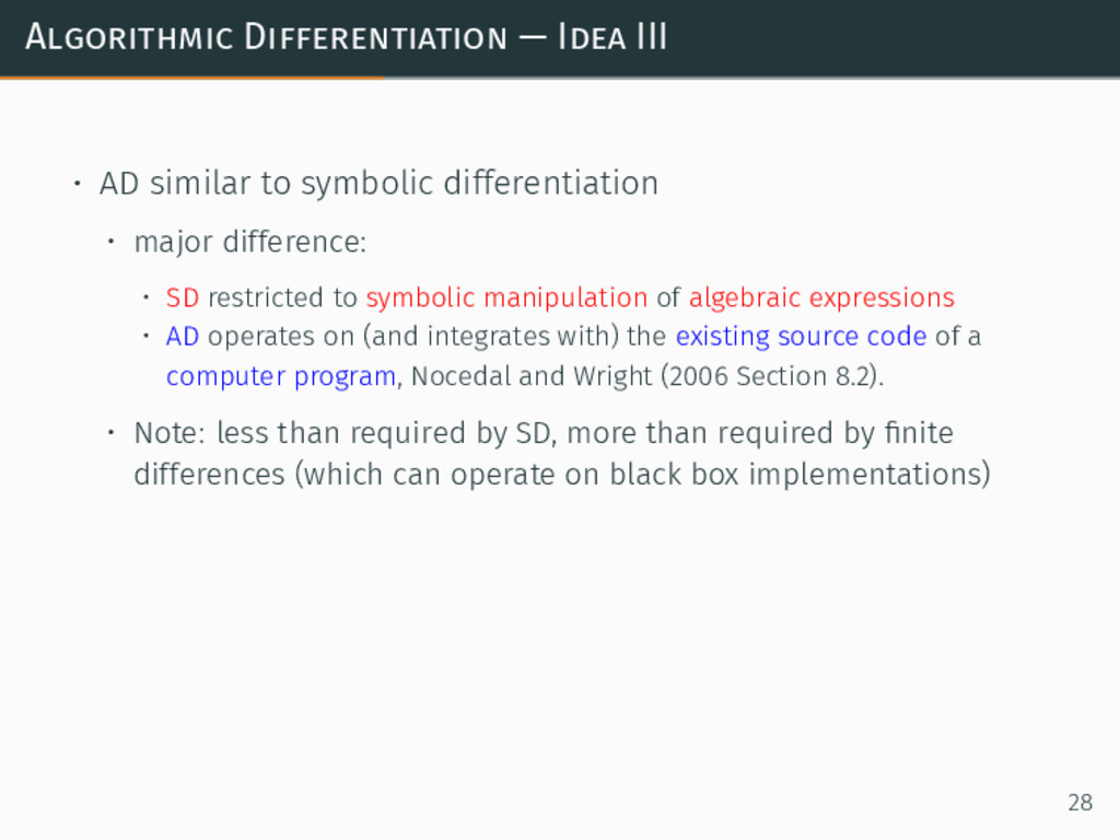
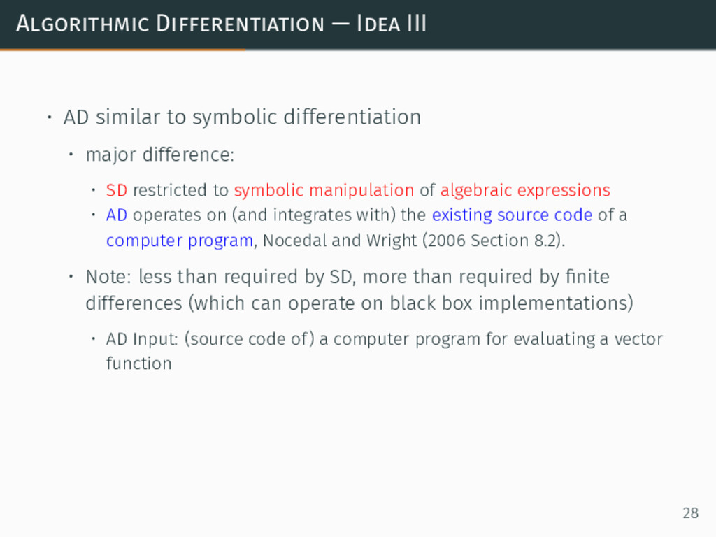
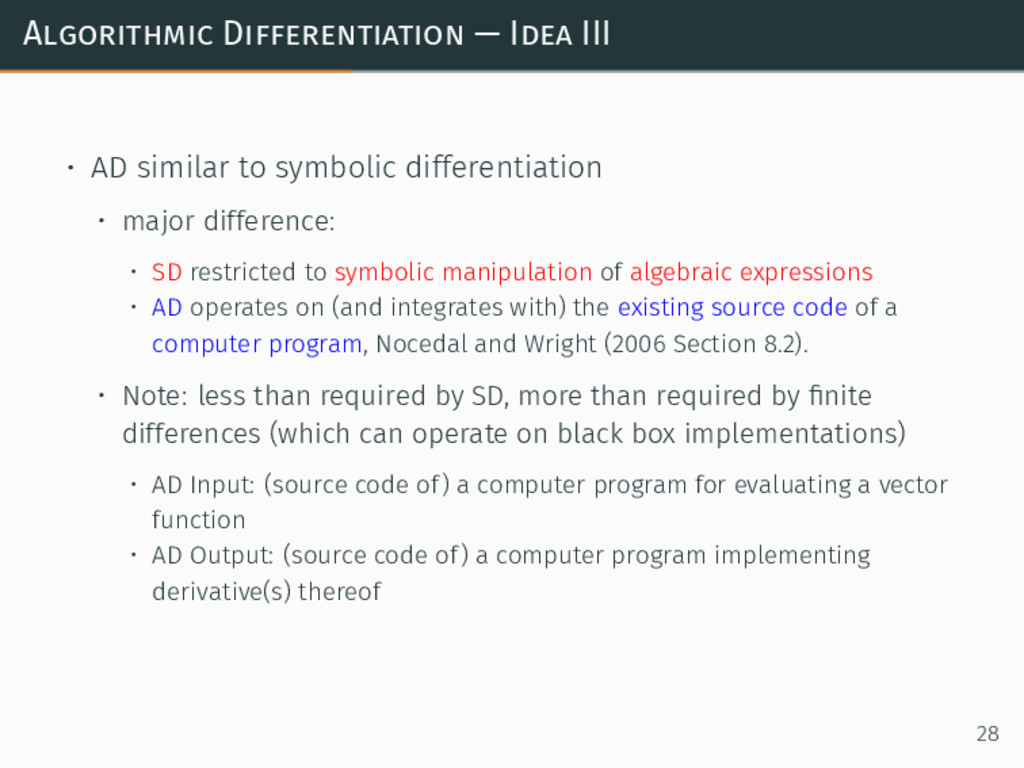
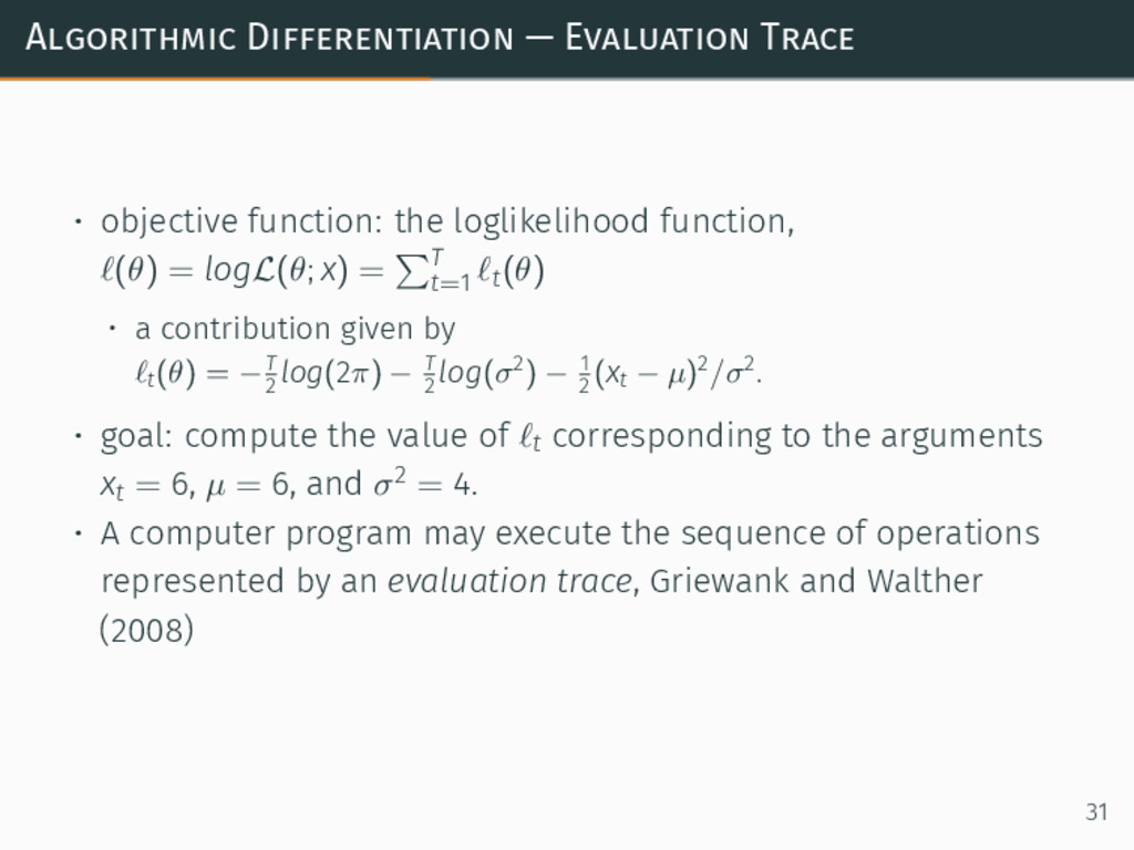
Algorithmic Differentiation (AD) enables automatic computation of the derivatives of a function implemented as a computer program. It's distinct from the numerical differentiation approximation methods (like finite differences), as it's exact to the maximum extent allowed by the machine precision. At the same time, it's free from the limitations of symbolic differentiation, since it works with actual computer programs (with branches, loops, allocations, and mutation) and not only pure, algebraic expressions.
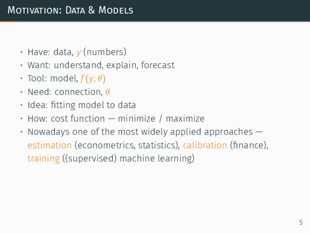
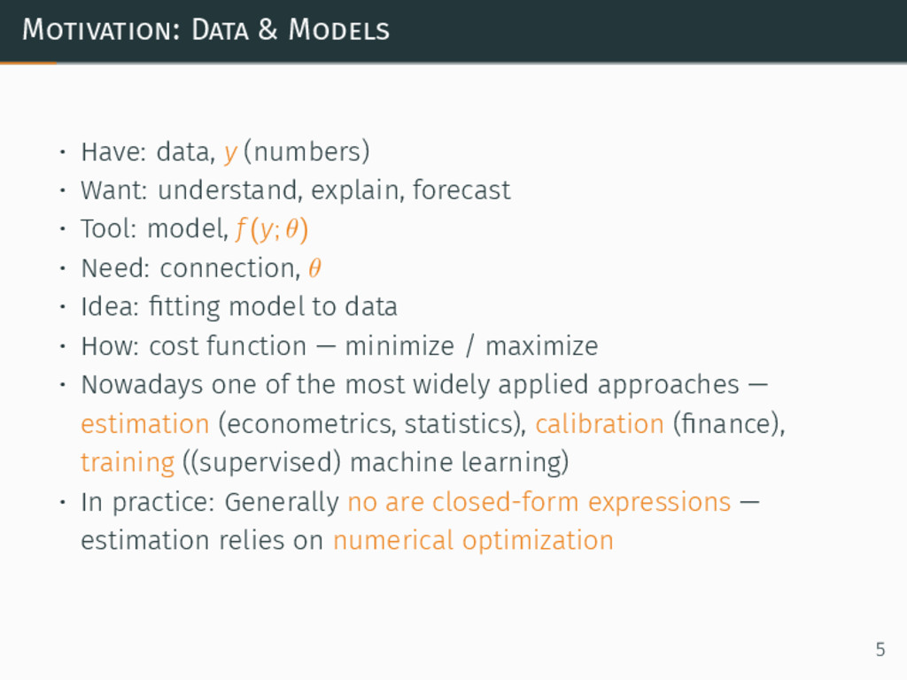
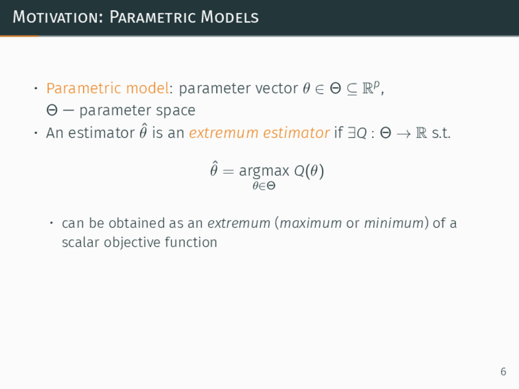
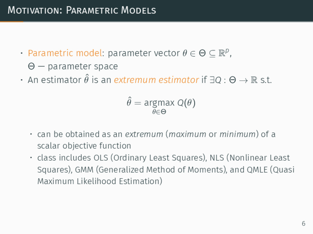
AD is useful to a wide range of applications – in particular, fitting models via extremum estimators (i.e., estimators obtained as extrema of the given cost functions). This includes calibrating financial models, training machine learning models, or estimating statistical (or econometric) models. Numerical optimization algorithms necessary for model fitting benefit greatly from the high precision of the gradient obtained using AD – with a direct impact on the ultimate results’ precision (more precise and stable parameter estimates, standard errors, confidence intervals).
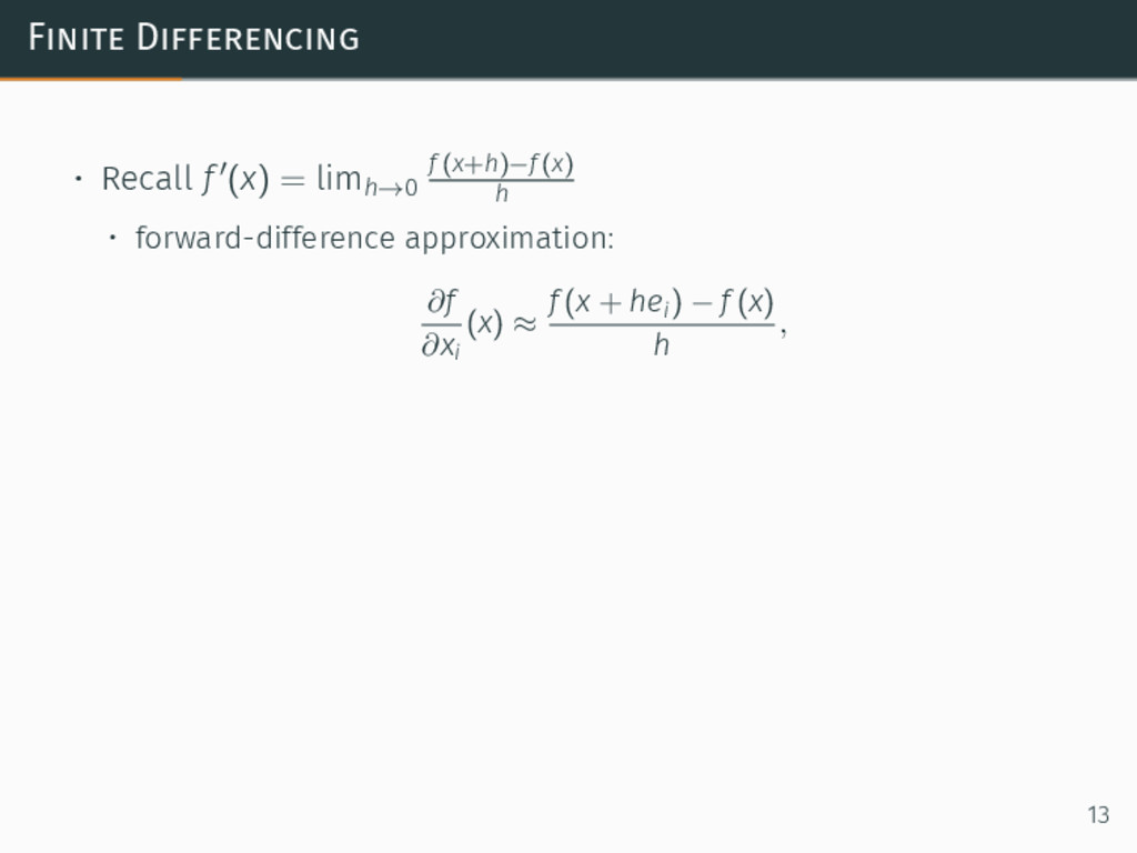
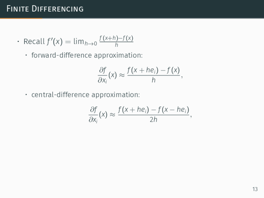
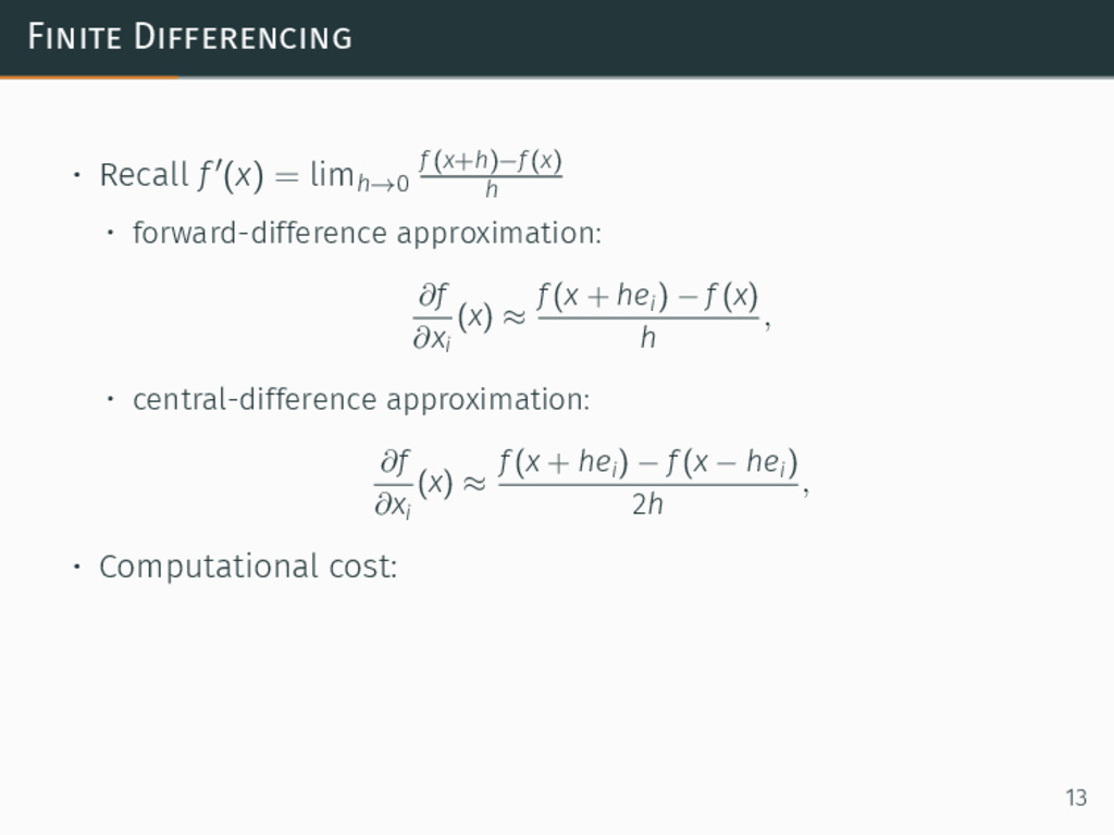
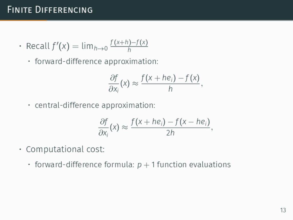
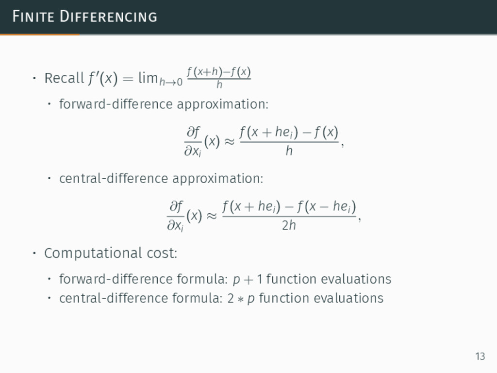
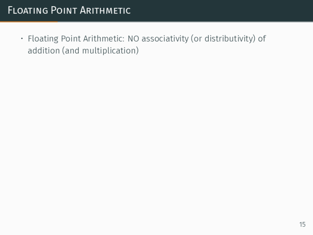
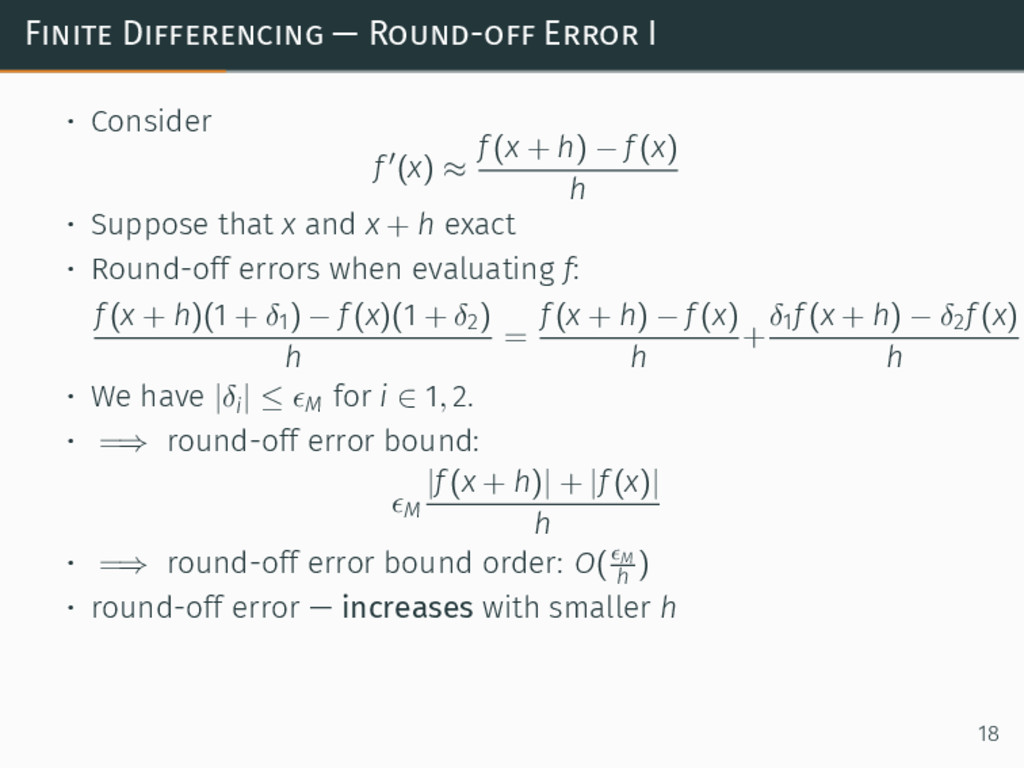
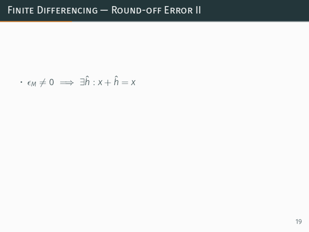
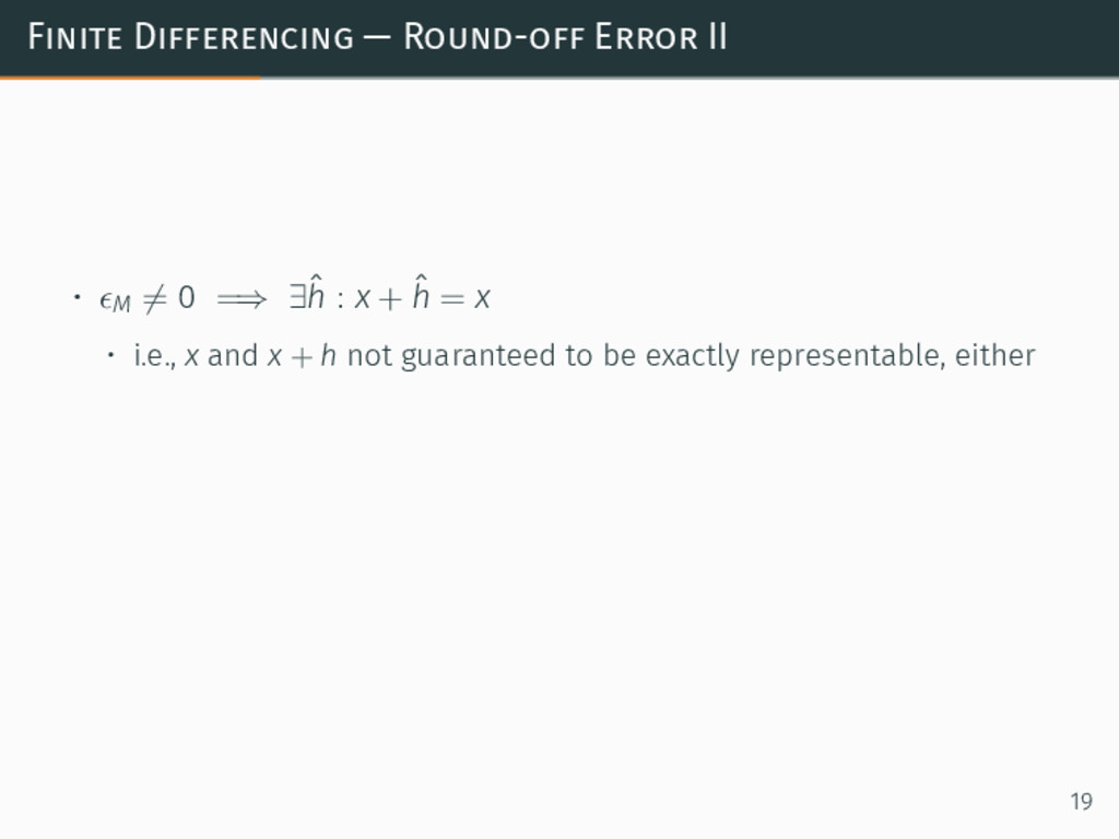
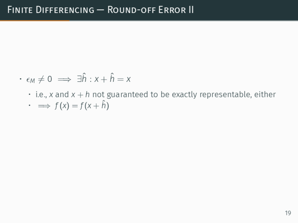
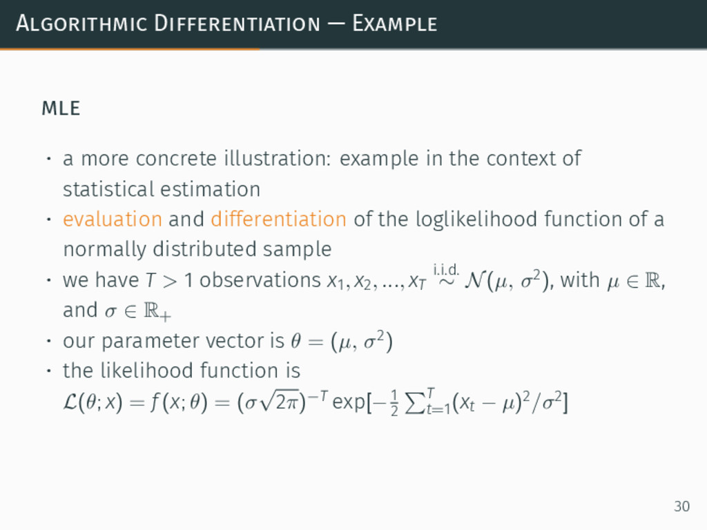
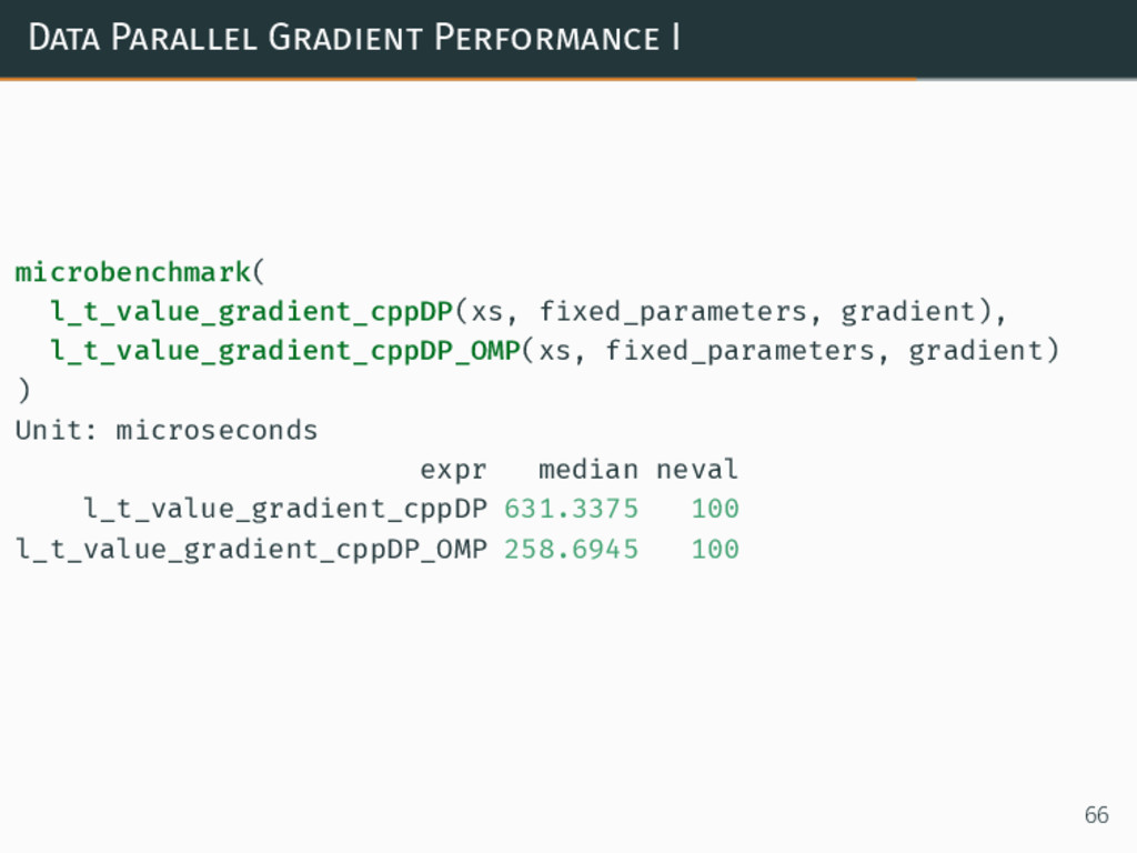
This lightning talk shows how to use AD – making the use of Eigen. We shall motivate the problem (including the issues with finite differences), introduce AD, and demonstrate its advantages over numerical approximations with a likelihood estimation example. We will end by speeding up the gradient computation via parallelization.
Last but not least: Recommended C++ software libraries and resources for anyone interested in finding out more about Algorithmic Differentiation.
![ExampleGaussianRcpp.cpp I // [[Rcpp::plugins("cpp11")]] #include <cstddef> // [[Rcpp::depends(BH)]] #include <boost/math/constants/constants.hpp>](https://files.speakerdeck.com/presentations/6e86dff8ec7b4203a041e756e9fc8fc1/slide_241.jpg)
![ExampleGaussianRcpp.cpp III // [[Rcpp::export]] double l_t_cpp(double xt, const Eigen::Map<Eigen::VectorXd> parameters)](https://files.speakerdeck.com/presentations/6e86dff8ec7b4203a041e756e9fc8fc1/slide_243.jpg)
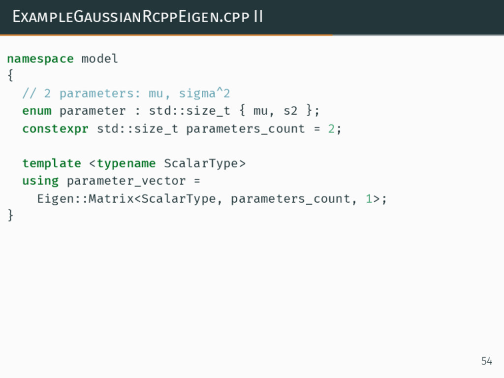
![ExampleGaussianRcppEigen.cpp I // [[Rcpp::plugins("cpp11")]] #include <cstddef> // [[Rcpp::depends(BH)]] #include <boost/math/constants/constants.hpp>](https://files.speakerdeck.com/presentations/6e86dff8ec7b4203a041e756e9fc8fc1/slide_245.jpg)
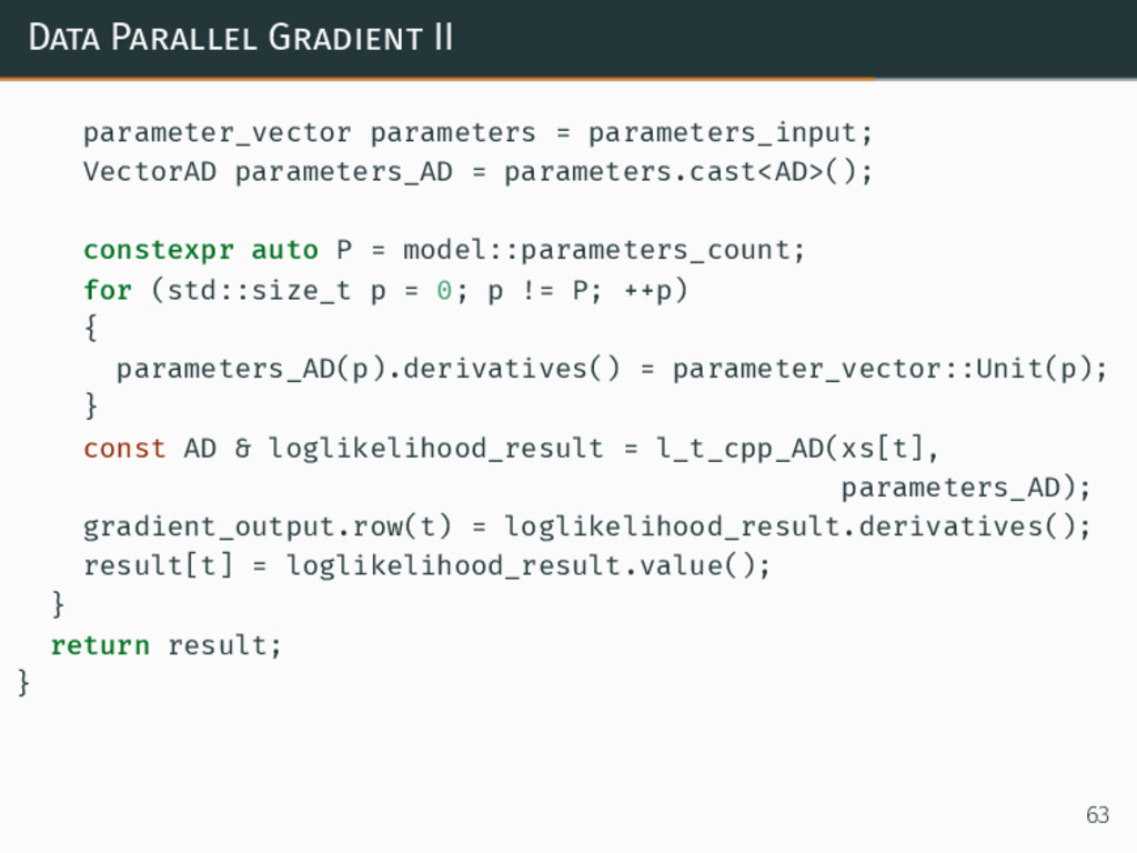
![Data Parallel Gradient I // [[Rcpp::export]] Eigen::VectorXd l_t_value_gradient_cppDP ( const](https://files.speakerdeck.com/presentations/6e86dff8ec7b4203a041e756e9fc8fc1/slide_254.jpg)
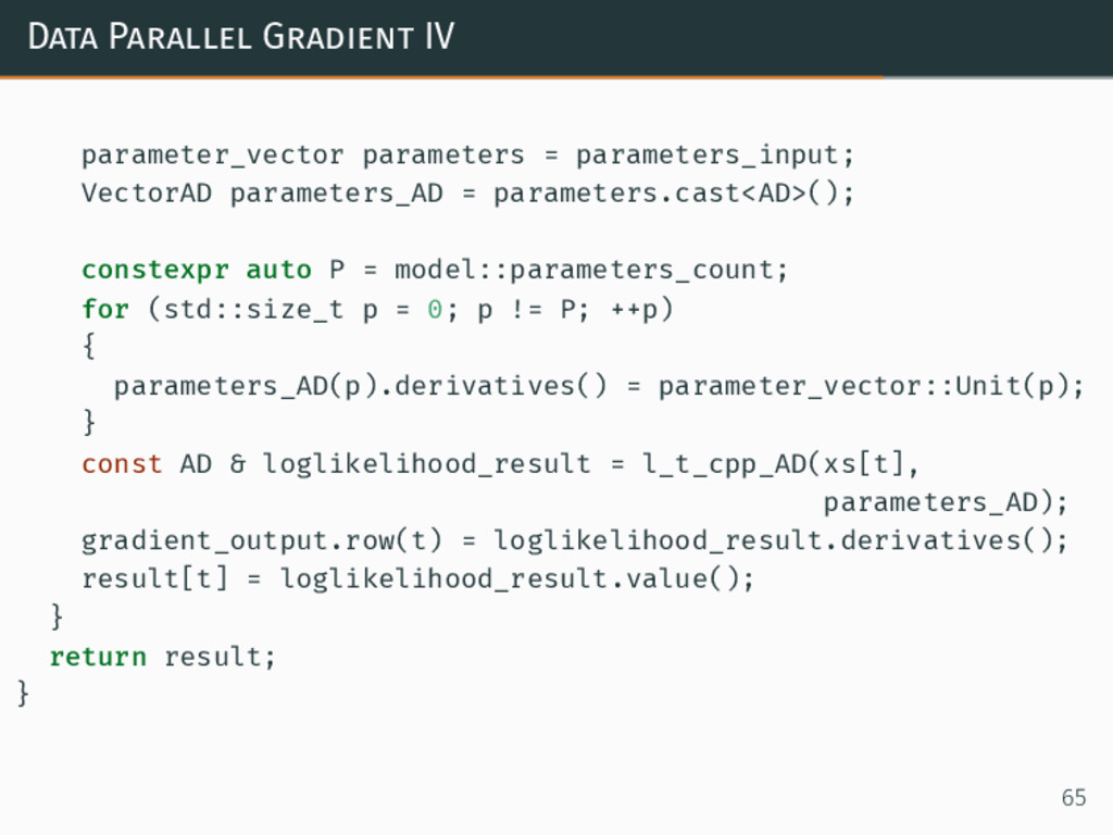
![Data Parallel Gradient III // [[Rcpp::export]] Eigen::VectorXd l_t_value_gradient_cppDP_OMP ( const](https://files.speakerdeck.com/presentations/6e86dff8ec7b4203a041e756e9fc8fc1/slide_256.jpg)