Symbolic Distillation of Neural Networks

I describe a general framework for distilling symbolic models from neural networks.

Transcript

1. Symbolic Distillation
 of Neural Networks Miles Cranmer Flatiron Institute University of Cambridge Princeton University
2. P2 ∝ a3 Kepler’s third law Kepler’s third law Empirical fi t: Problem:
3. P2 ∝ a3 Kepler’s third law Newton’s law of gravitation, 
 to explain it Kepler’s third law Empirical fi t: Problem:
4. P2 ∝ a3 Kepler’s third law Newton’s law of gravitation, 
 to explain it Kepler’s third law Planck’s law B = 2hν3 c2 ( exp ( hν kB T) − 1 ) −1 Empirical fi t: Problem:
5. P2 ∝ a3 Kepler’s third law Newton’s law of gravitation, 
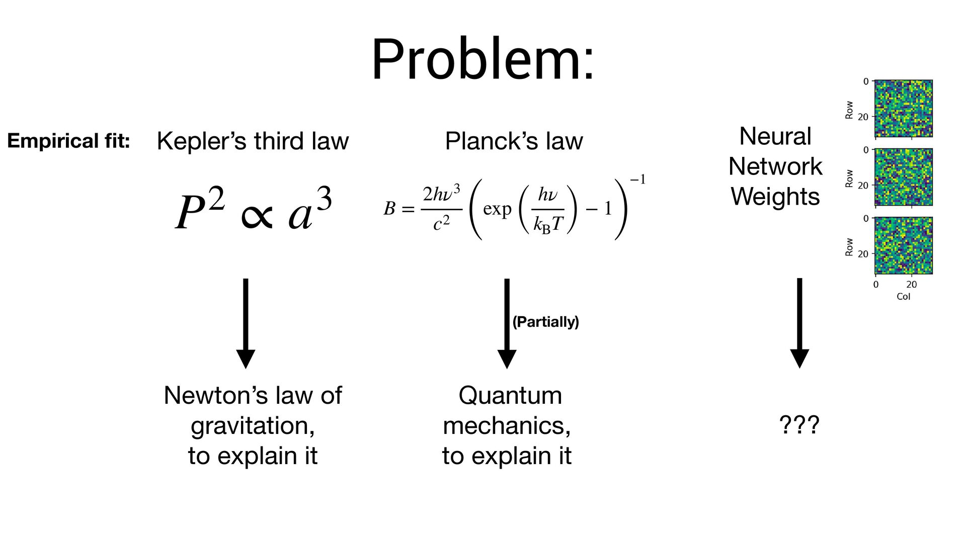
 to explain it Kepler’s third law Planck’s law B = 2hν3 c2 ( exp ( hν kB T) − 1 ) −1 Empirical fi t: Quantum mechanics, 
 to explain it (Partially) Problem:
6. P2 ∝ a3 Kepler’s third law Newton’s law of gravitation, 
 to explain it Kepler’s third law Planck’s law B = 2hν3 c2 ( exp ( hν kB T) − 1 ) −1 Empirical fi t: Neural 
 Network
 Weights Quantum mechanics, 
 to explain it (Partially) Problem:
7. P2 ∝ a3 Kepler’s third law Newton’s law of gravitation, 
 to explain it Kepler’s third law Planck’s law B = 2hν3 c2 ( exp ( hν kB T) − 1 ) −1 Empirical fi t: Neural 
 Network
 Weights ??? Quantum mechanics, 
 to explain it (Partially) Problem:
8. What I want: I want ML to create models in a language* I can understand** → Insights into existing models → Understand biases, learned shortcuts → Can place stronger priors on learned functions
9. Industry version of interpretability • All revolves around saliency or feature importance • Consider the “saliency map” Omeiza et al., 2019
10. Industry version of interpretability • All revolves around saliency or feature importance • Consider the “saliency map” Omeiza et al., 2019
11. (- Feynman’s blackboard)
12. Science already has a modeling language
13. Science already has a modeling language Computer Vision
14. Science already has a modeling language Computer Vision ???
15. Science already has a modeling language Computer Vision Science ???
16. Science already has a modeling language Computer Vision Science ???
18. We should build interpretations in this existing language: mathematical expressions!
19. Symbolic regression • Symbolic regression fi nds analytic expressions to fi t a dataset. • (~another name for "program synthesis”) • Pioneering work by Langley et al., 1980s; Koza et al., 1990s; Lipson et al., 2000s
20. How can I try this?
21. How can I try this? • Open-source
22. How can I try this? • Open-source • Extensible Python API compatible with scikit-learn
23. How can I try this? • Open-source • Extensible Python API compatible with scikit-learn • Can be distributed over 1000s of cores
 (w/ slurm, PBS, LSF, or Kubernetes)
24. How can I try this? • Open-source • Extensible Python API compatible with scikit-learn • Can be distributed over 1000s of cores
 (w/ slurm, PBS, LSF, or Kubernetes) • Custom operators, losses, constraints
27. Great! But, there’s a problem:
28. Great! But, there’s a problem: • Genetic algorithms, like PySR, scale terribly with expression complexity.
29. Great! But, there’s a problem: • Genetic algorithms, like PySR, scale terribly with expression complexity. • One must search over:
30. Great! But, there’s a problem: • Genetic algorithms, like PySR, scale terribly with expression complexity. • One must search over: • (permutations of operators) x (permutations of variables + possible constants)
31. Great! But, there’s a problem: • Genetic algorithms, like PySR, scale terribly with expression complexity. • One must search over: • (permutations of operators) x (permutations of variables + possible constants)
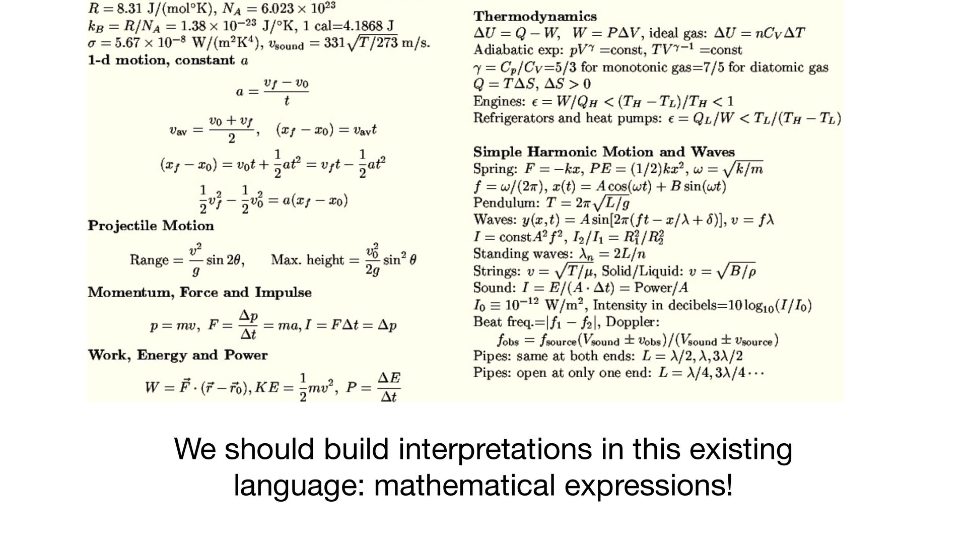
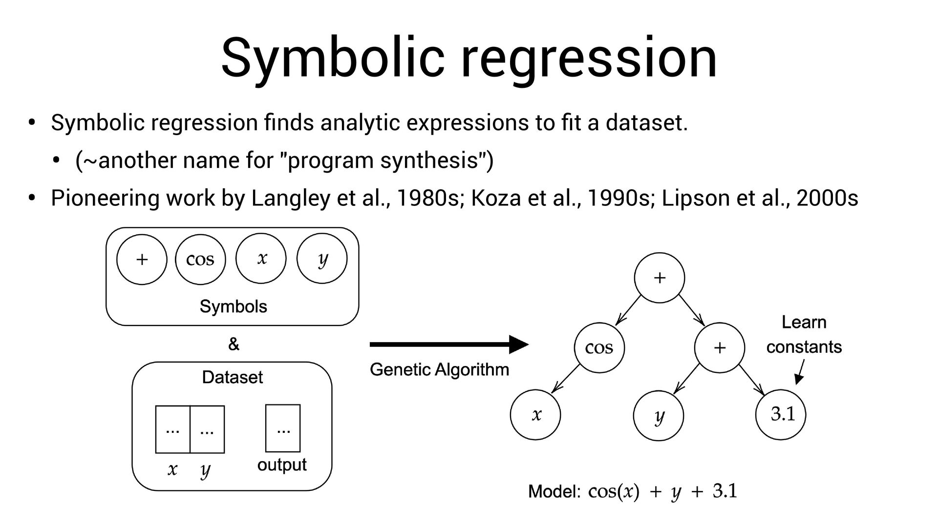
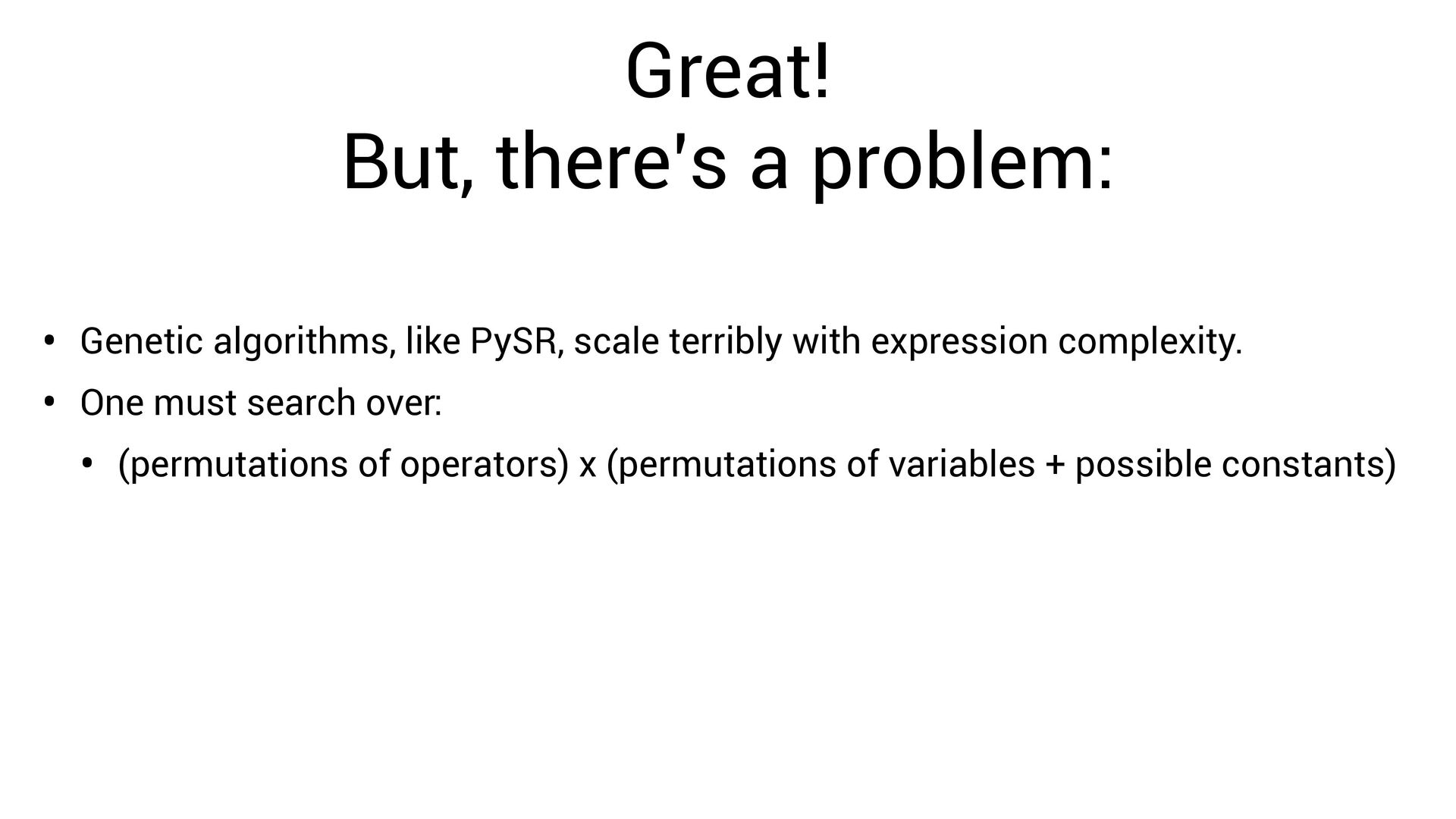
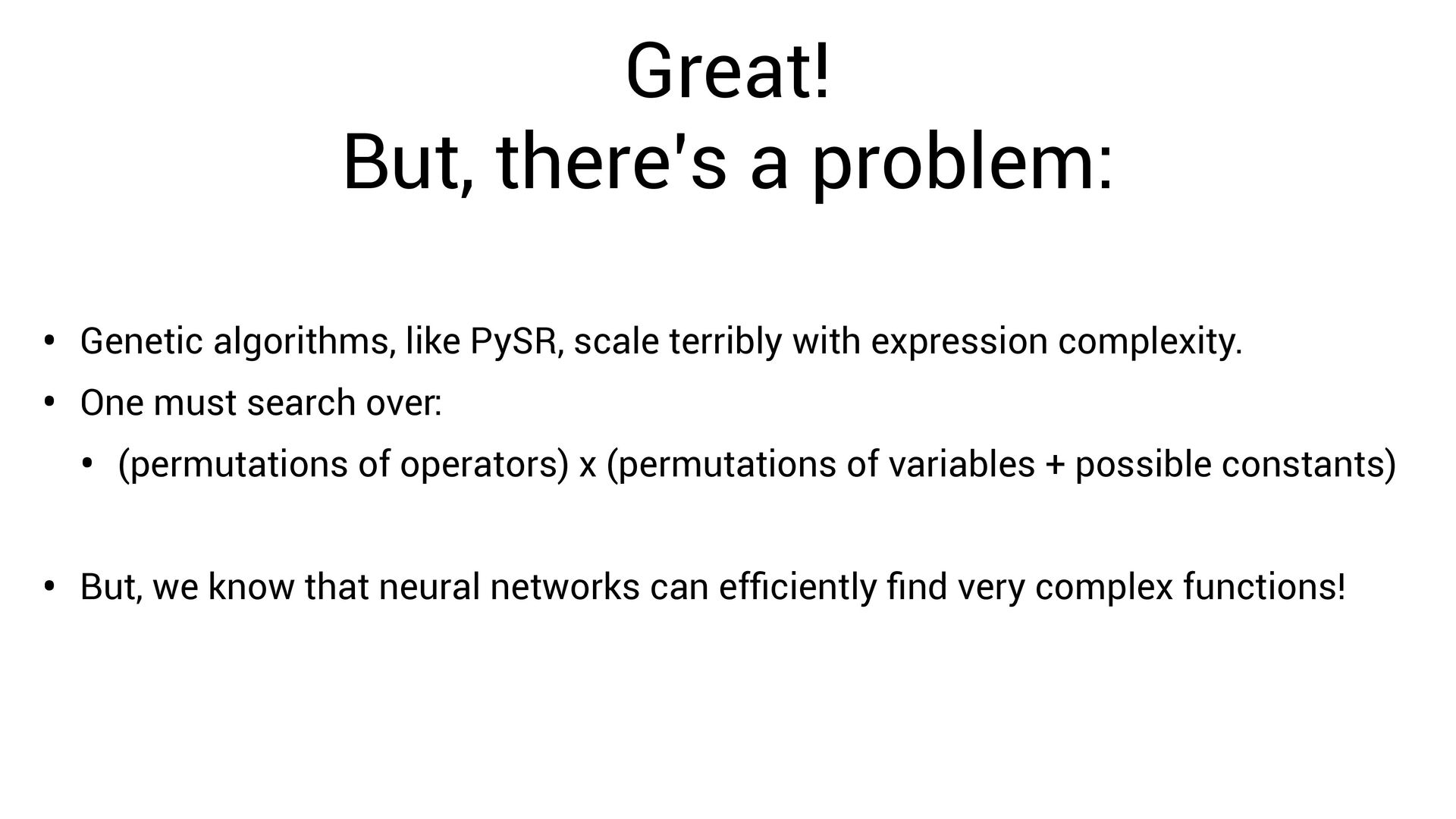
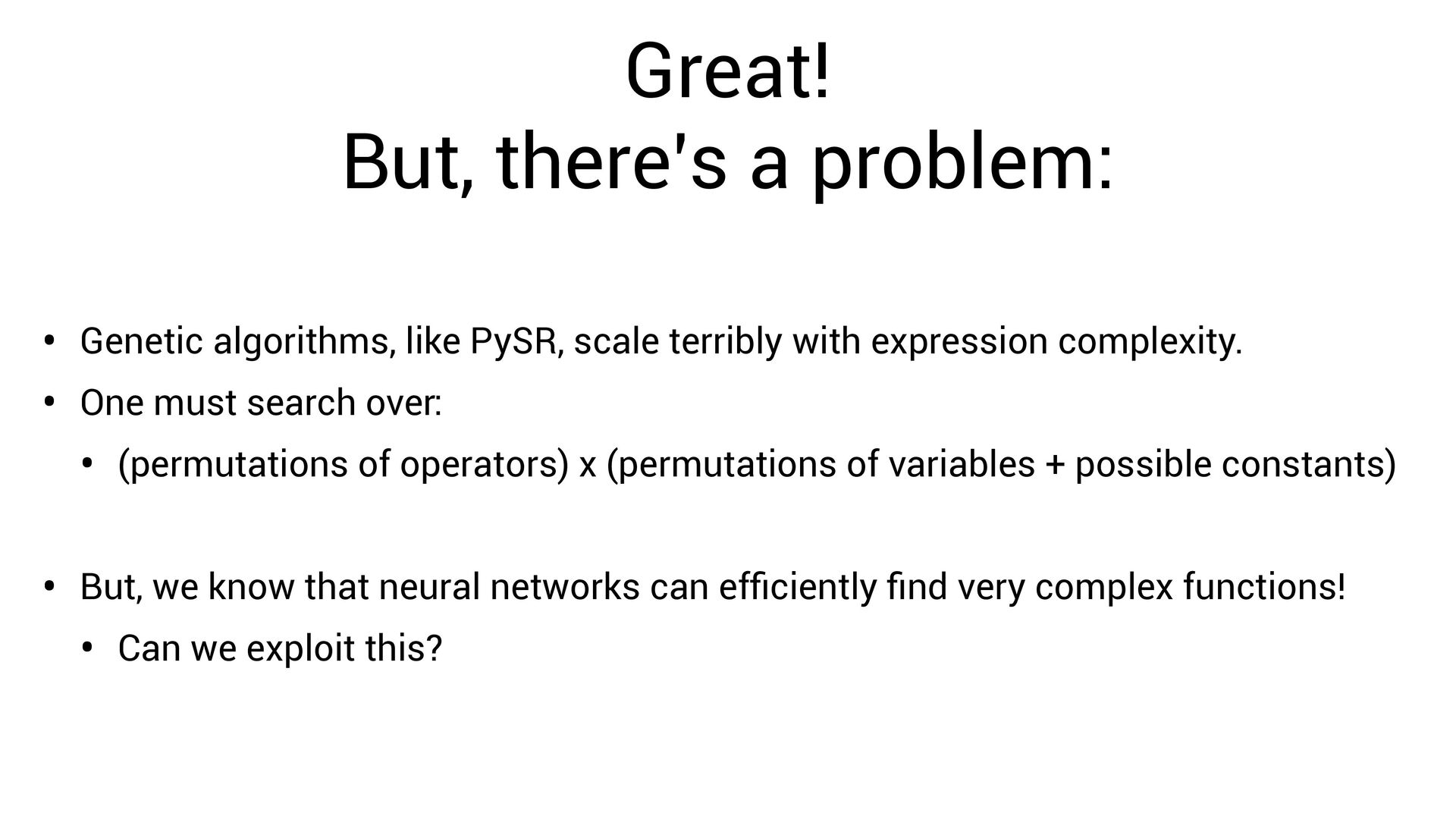
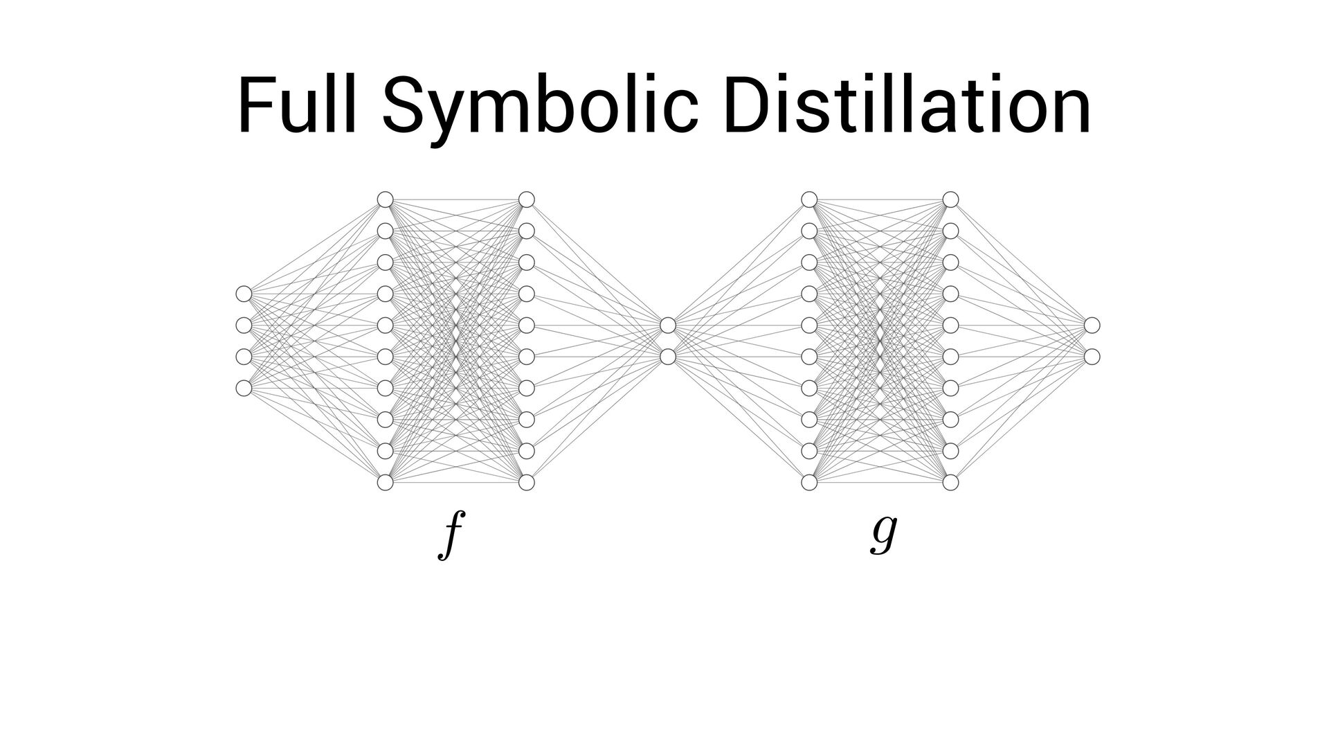
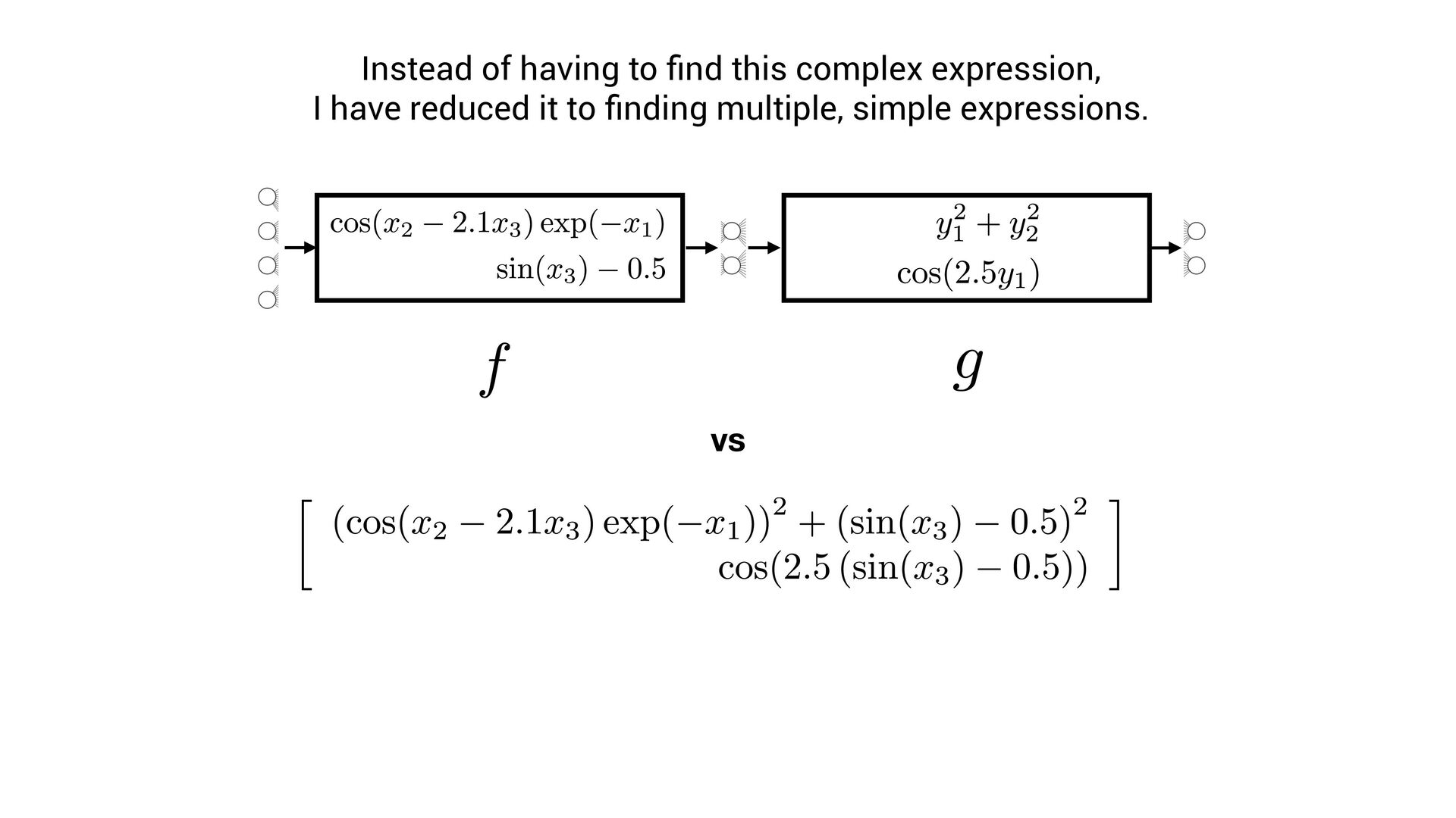
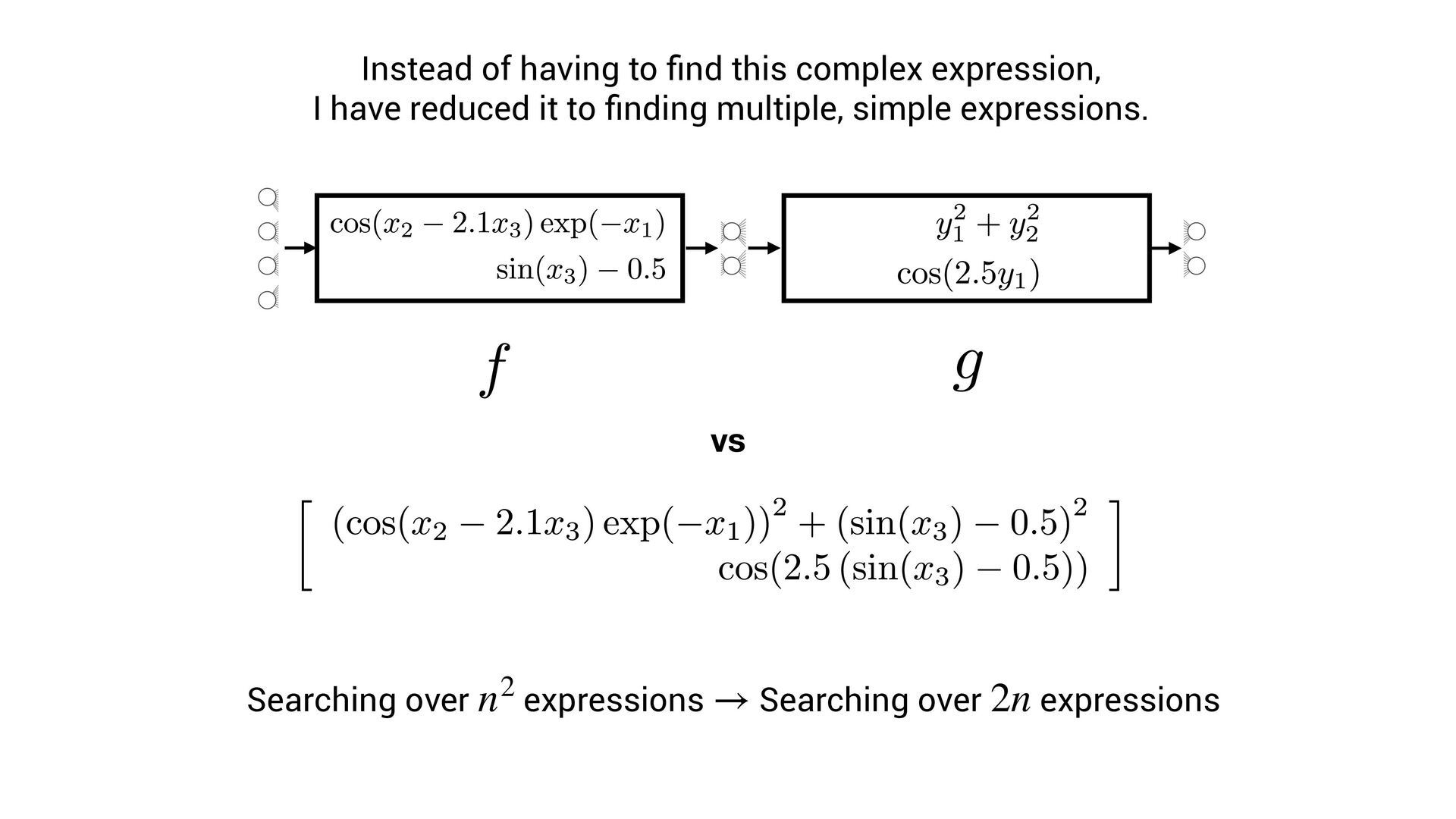
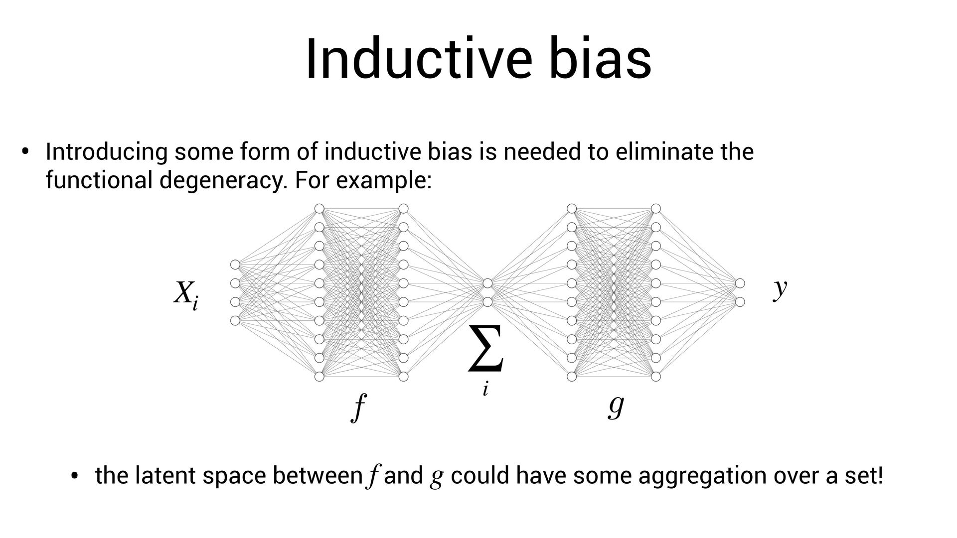
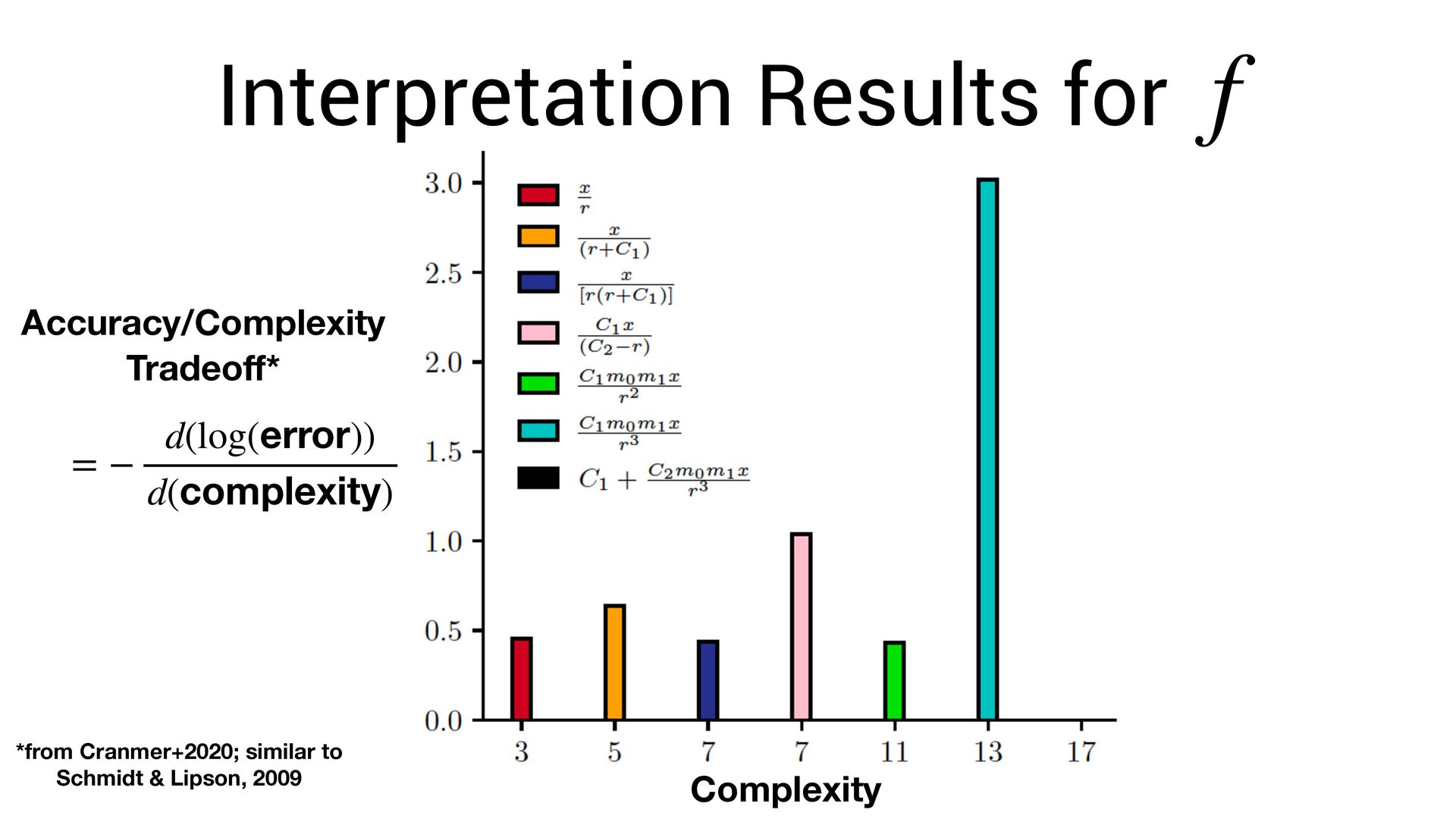
32. Great! But, there’s a problem: • Genetic algorithms, like PySR, scale terribly with expression complexity. • One must search over: • (permutations of operators) x (permutations of variables + possible constants) • But, we know that neural networks can ef fi ciently fi nd very complex functions!
33. Great! But, there’s a problem: • Genetic algorithms, like PySR, scale terribly with expression complexity. • One must search over: • (permutations of operators) x (permutations of variables + possible constants) • But, we know that neural networks can ef fi ciently fi nd very complex functions! • Can we exploit this?
34. Symbolic Distillation Neural network
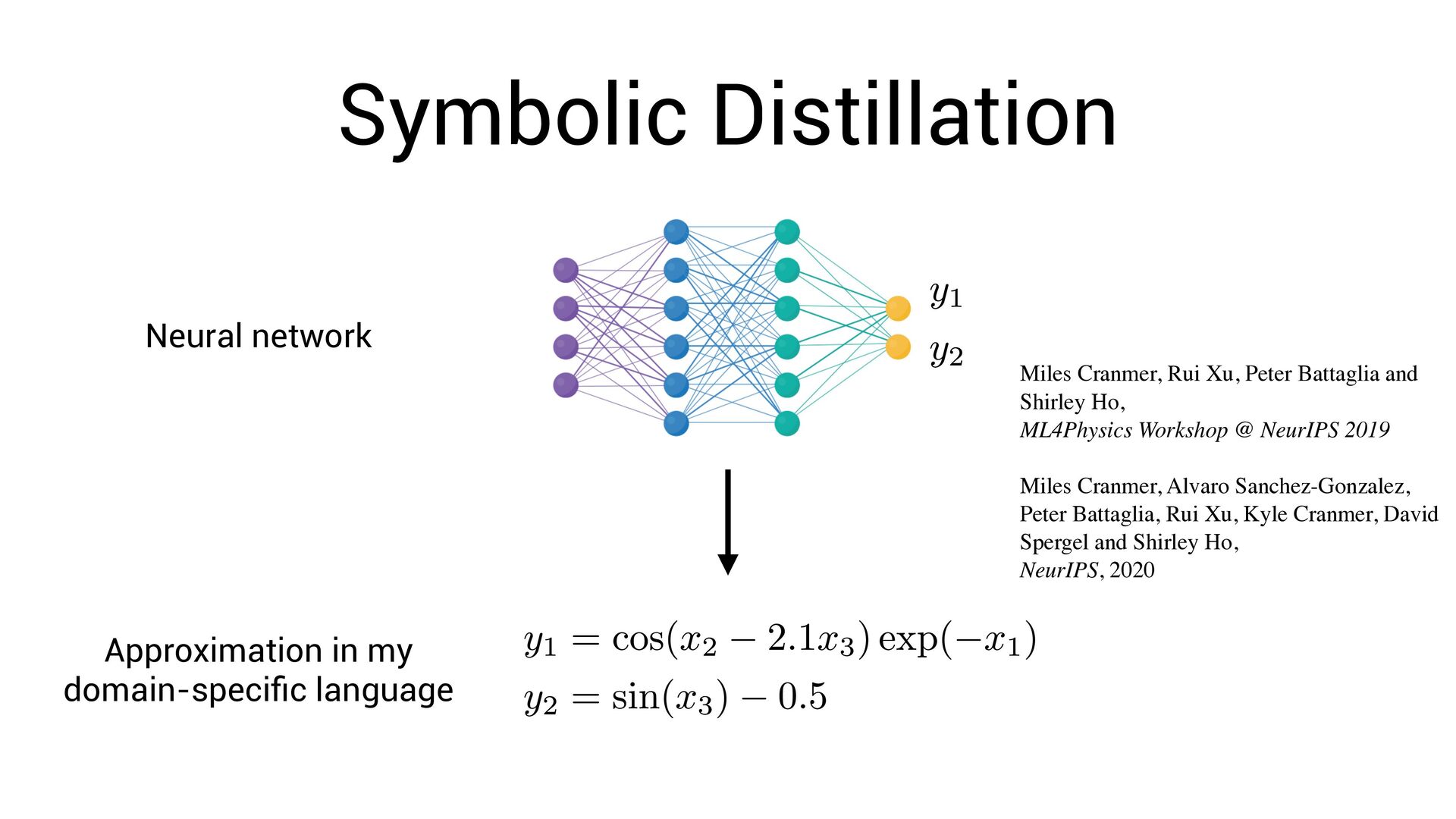
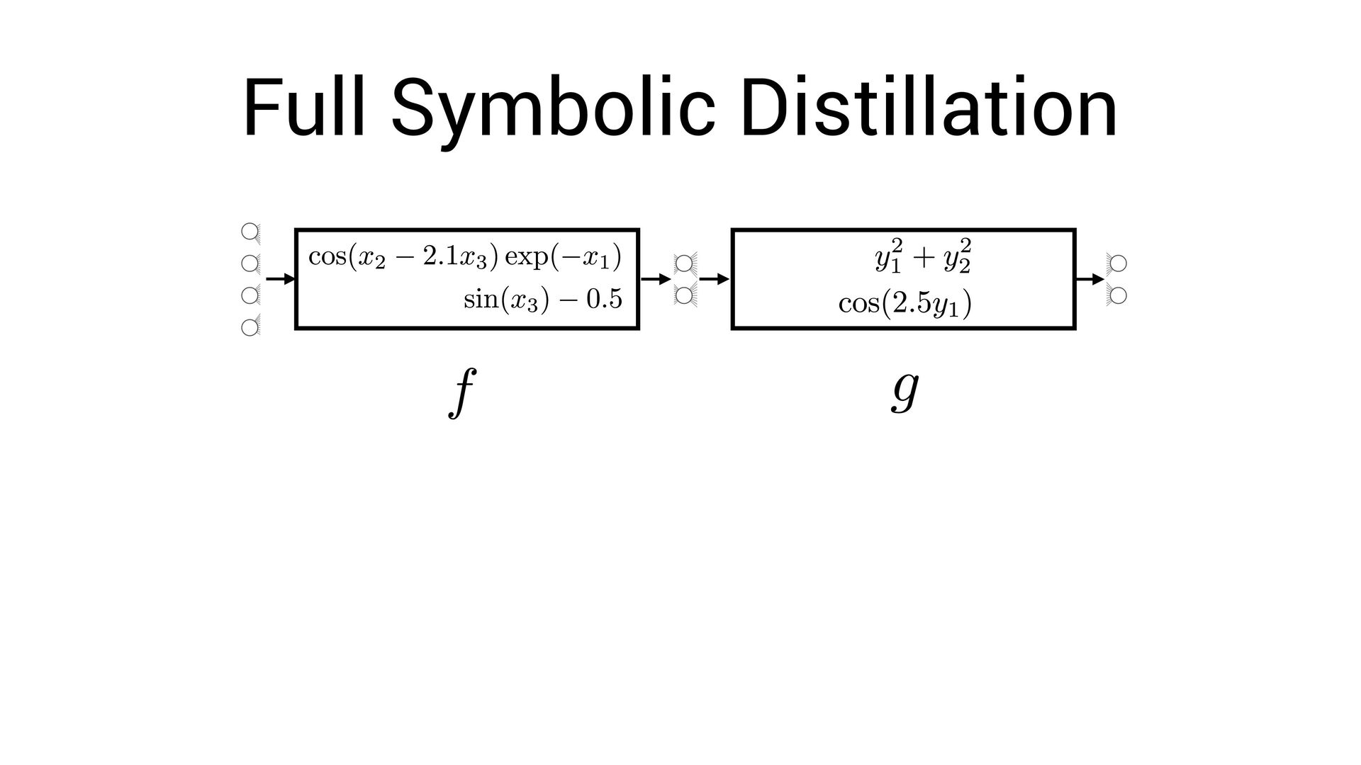
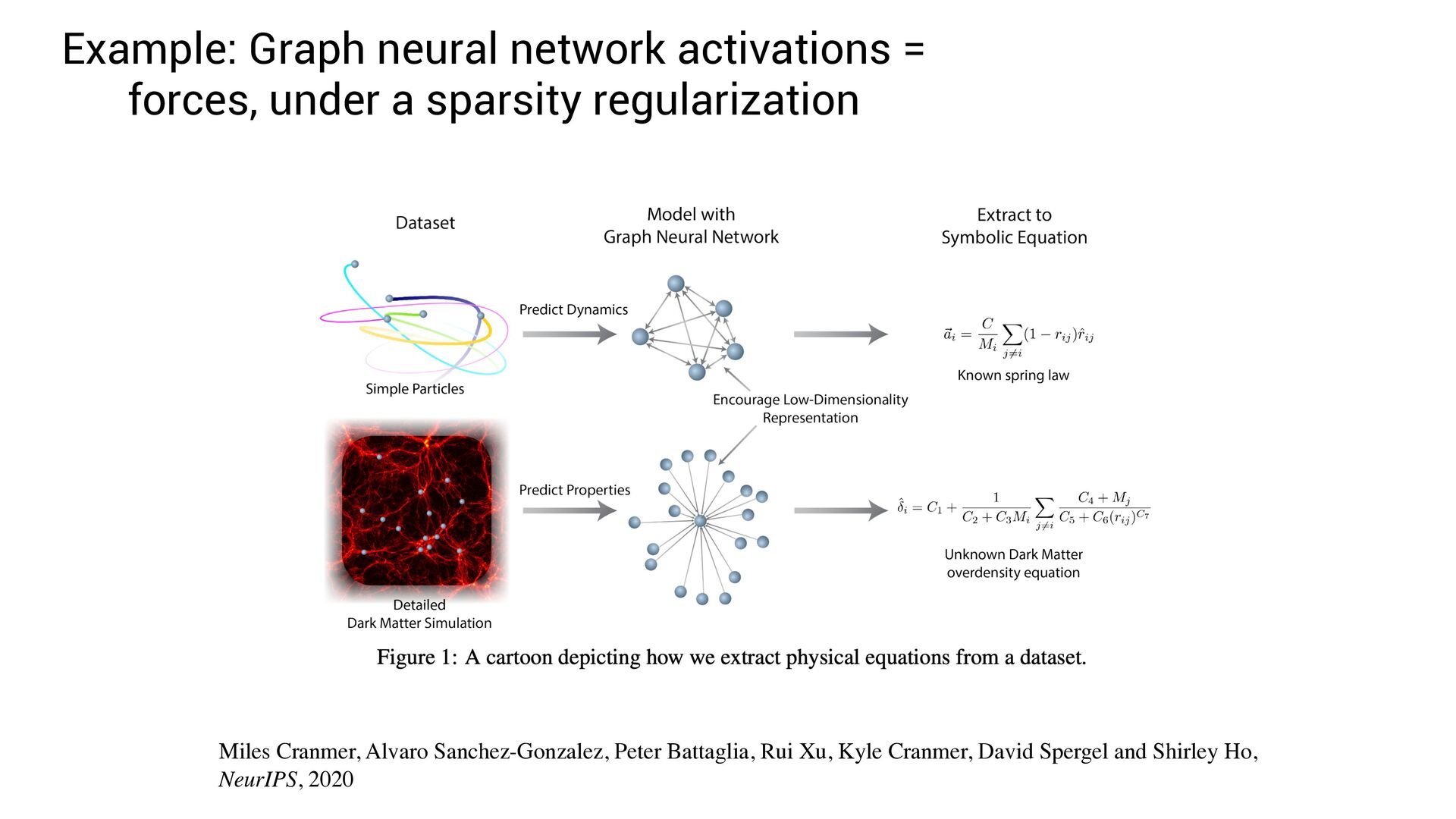
35. Symbolic Distillation Neural network Approximation in my domain-speci fi c language Miles Cranmer, Rui Xu, Peter Battaglia and Shirley Ho, 
 ML4Physics Workshop @ NeurIPS 2019 Miles Cranmer, Alvaro Sanchez-Gonzalez, Peter Battaglia, Rui Xu, Kyle Cranmer, David Spergel and Shirley Ho, 
 NeurIPS, 2020
36. How this works: 1. Train NN normally, 
 and freeze parameters.
37. How this works: 1. Train NN normally, 
 and freeze parameters. 2. Record input/outputs of
 network over training set.
38. How this works: 1. Train NN normally, 
 and freeze parameters. 2. Record input/outputs of
 network over training set. PySR 3. Fit the input/outputs of the neural network with PySR
39. Analogy “Taylor expanding the Neural Network”
40. Analogy “Taylor expanding the Neural Network”
41. Full Symbolic Distillation
42. Full Symbolic Distillation Learns features? Uses features
 for calculation?
43. Full Symbolic Distillation Learns features? Uses features
 for calculation?
44. Full Symbolic Distillation
45. Full Symbolic Distillation Re-train , to pick up any errors
 in the approximation of g f 🔄
46. Full Symbolic Distillation
47. Full Symbolic Distillation
48. Full Symbolic Distillation
49. Full Symbolic Distillation
50. Full Symbolic Distillation (g ∘ f)(x1 , x2 , x3 , x4 ) =
51. Full Symbolic Distillation (g ∘ f)(x1 , x2 , x3 , x4 ) = Fully-interpretable approximation of the original neural network!
52. Full Symbolic Distillation (g ∘ f)(x1 , x2 , x3 , x4 ) = Fully-interpretable approximation of the original neural network!
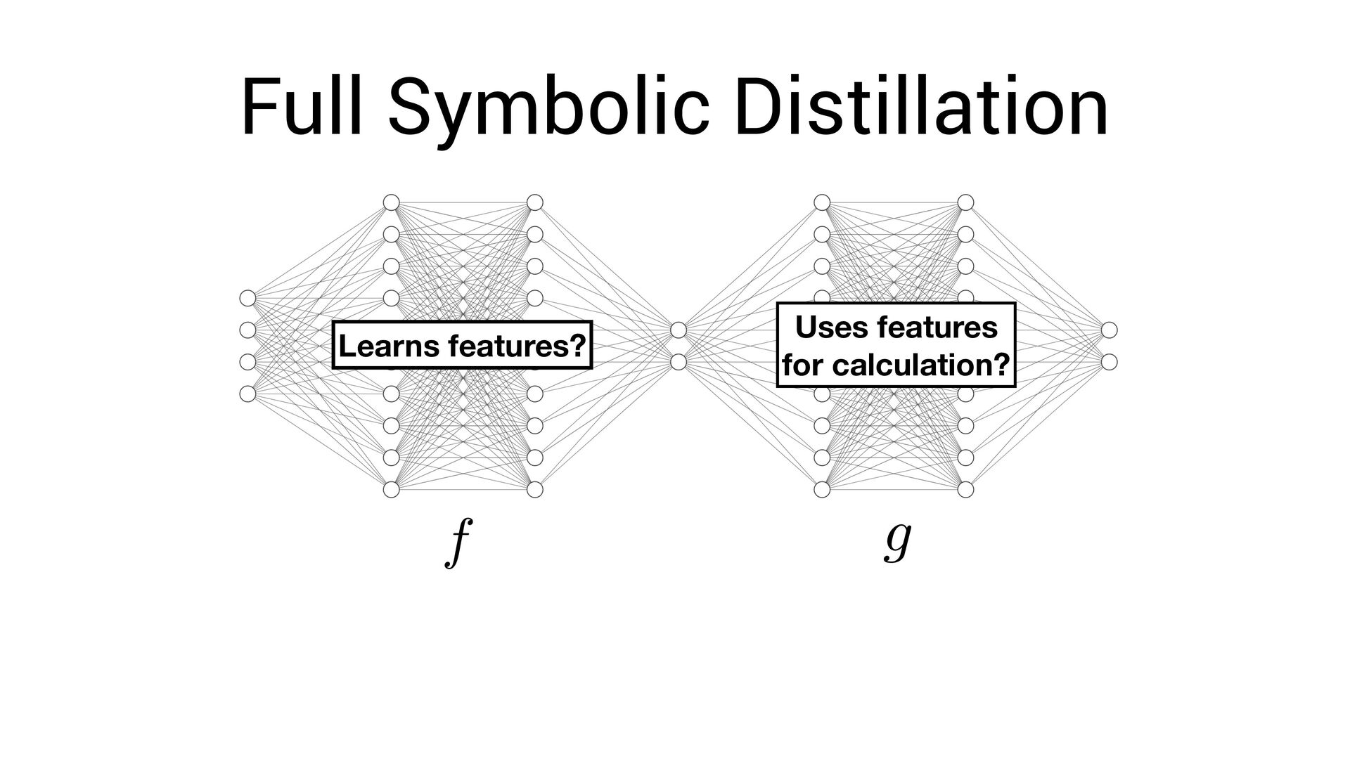
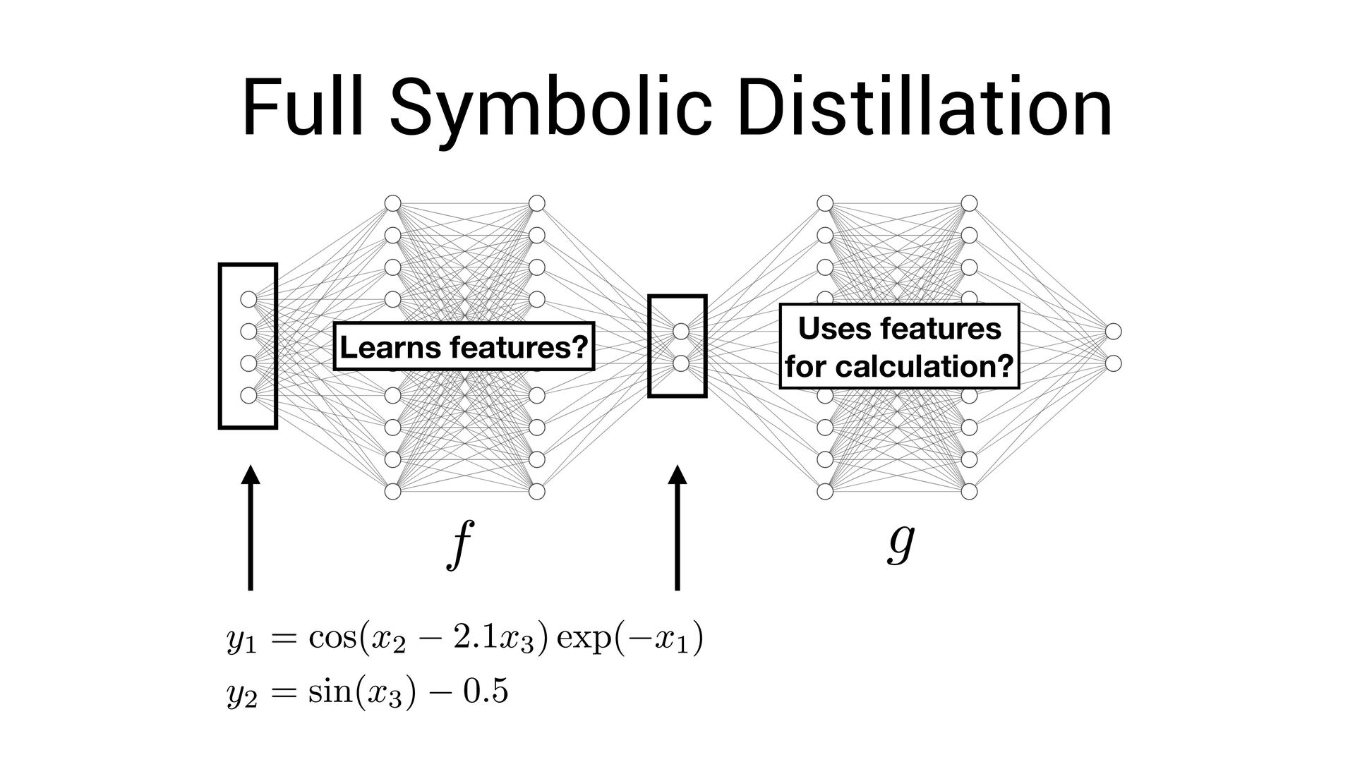
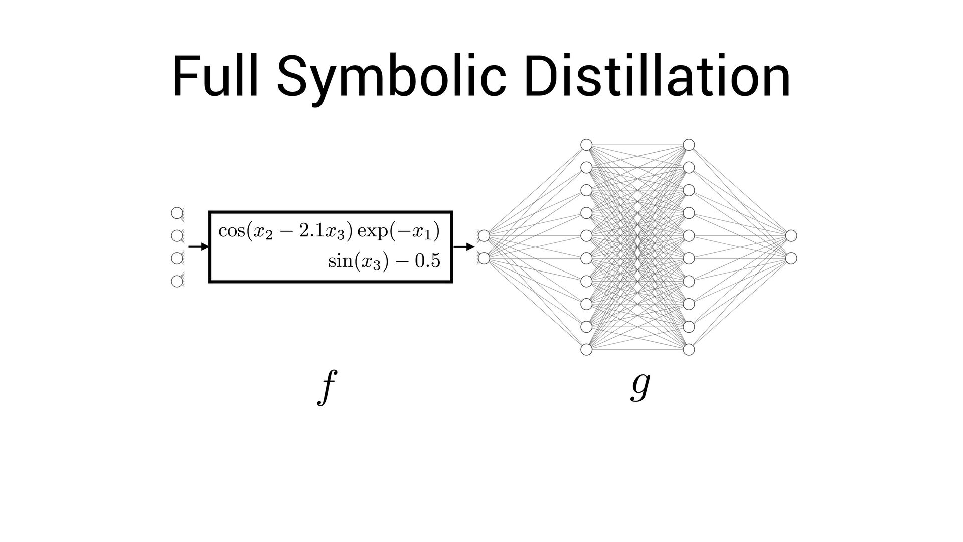
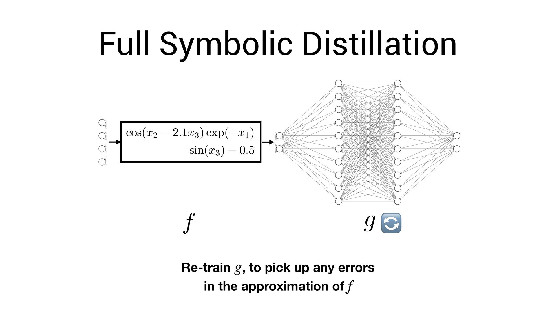
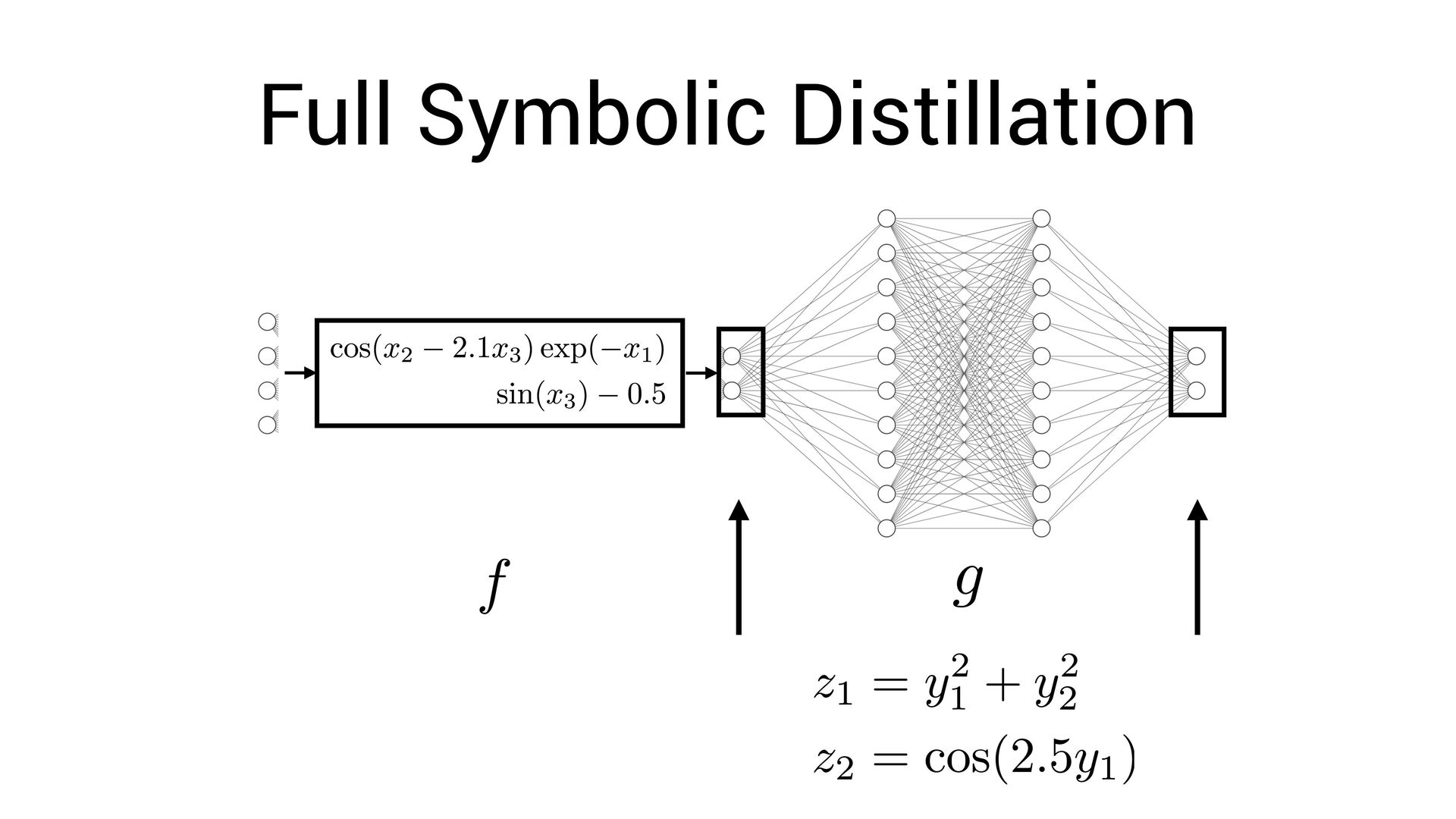
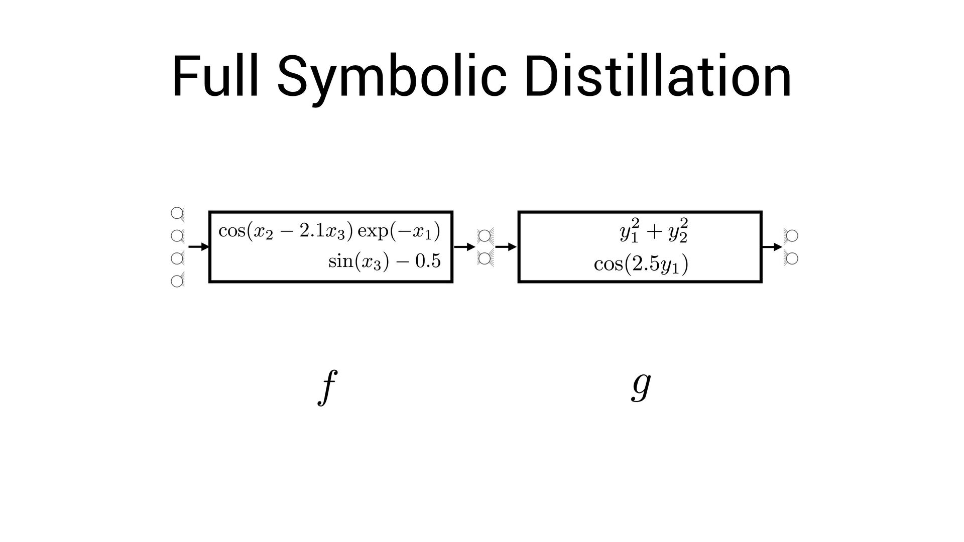
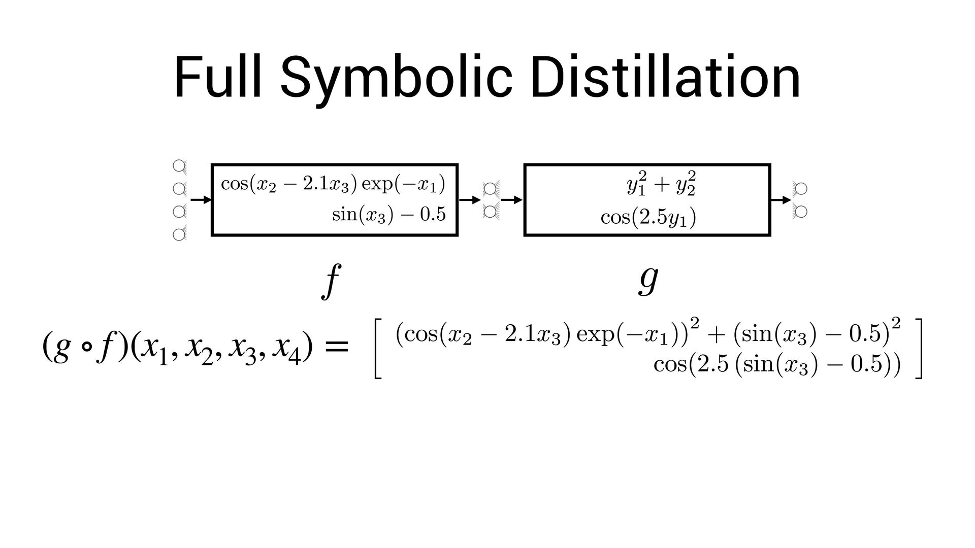
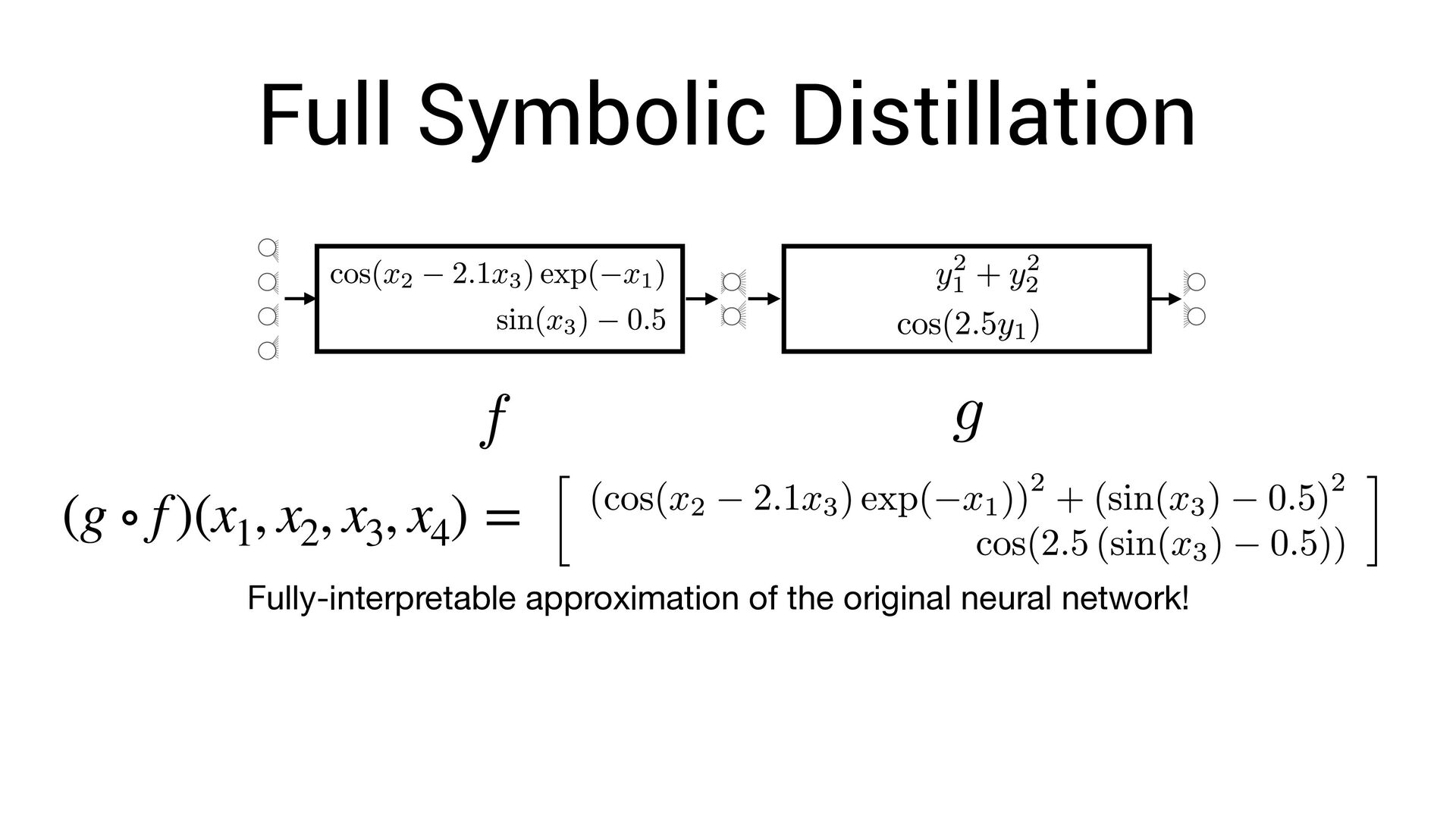
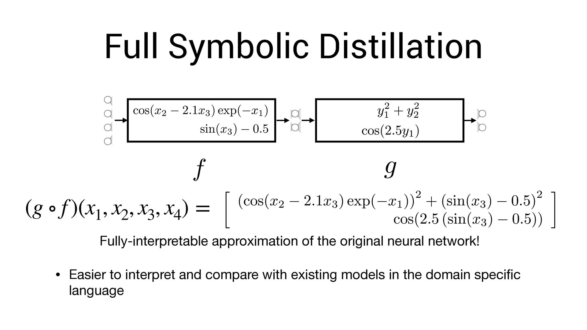
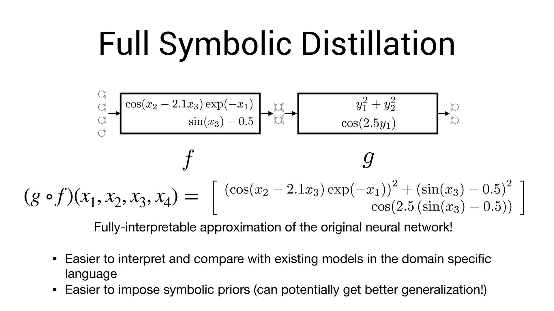
53. Full Symbolic Distillation (g ∘ f)(x1 , x2 , x3 , x4 ) = Fully-interpretable approximation of the original neural network! • Easier to interpret and compare with existing models in the domain speci fi c language
54. Full Symbolic Distillation (g ∘ f)(x1 , x2 , x3 , x4 ) = Fully-interpretable approximation of the original neural network! • Easier to interpret and compare with existing models in the domain speci fi c language • Easier to impose symbolic priors (can potentially get better generalization!)
55. vs Instead of having to fi nd this complex expression, 
 I have reduced it to fi nding multiple, simple expressions.
56. Searching over expressions Searching over expressions n2 → 2n vs Instead of having to fi nd this complex expression, 
 I have reduced it to fi nding multiple, simple expressions.
57. What about the functional degeneracy? Any over-complicated functional form that learns, could invert! f g
58. Xi y Inductive bias • Introducing some form of inductive bias is needed to eliminate the functional degeneracy. For example:
59. Xi y Inductive bias • Introducing some form of inductive bias is needed to eliminate the functional degeneracy. For example: • the latent space between and could have some aggregation over a set! f g ∑ i
60. Inductive bias
61. Inductive bias • Other inductive biases to eliminate the degeneracy:
62. Inductive bias • Other inductive biases to eliminate the degeneracy: • Sparsity on latent space ( fewer equations, fewer variables) ⇒
63. Inductive bias • Other inductive biases to eliminate the degeneracy: • Sparsity on latent space ( fewer equations, fewer variables) ⇒ • (Also see related work of Sebastian Wetzel & Roger Melko; and Steve Brunton & Nathan Kutz!)
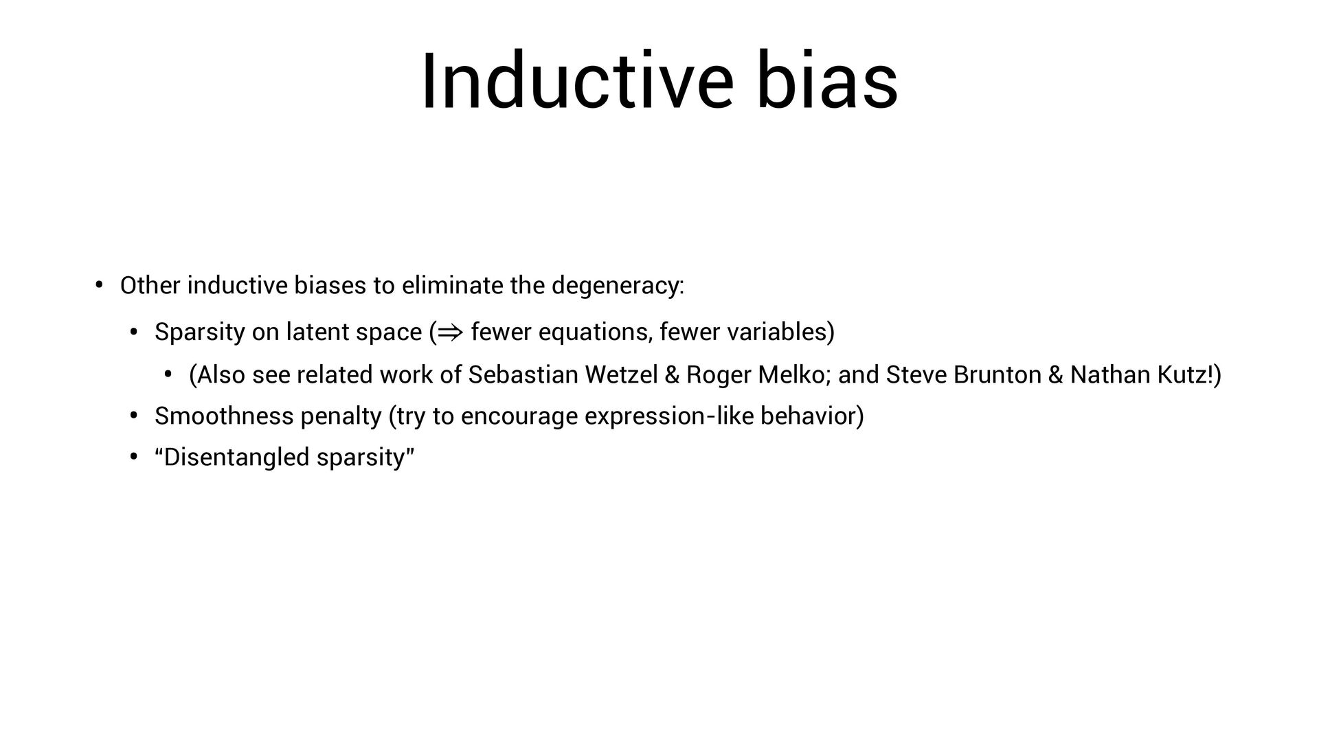
64. Inductive bias • Other inductive biases to eliminate the degeneracy: • Sparsity on latent space ( fewer equations, fewer variables) ⇒ • (Also see related work of Sebastian Wetzel & Roger Melko; and Steve Brunton & Nathan Kutz!) • Smoothness penalty (try to encourage expression-like behavior)
65. Inductive bias • Other inductive biases to eliminate the degeneracy: • Sparsity on latent space ( fewer equations, fewer variables) ⇒ • (Also see related work of Sebastian Wetzel & Roger Melko; and Steve Brunton & Nathan Kutz!) • Smoothness penalty (try to encourage expression-like behavior) • “Disentangled sparsity”
66. Miles Cranmer, Can Cui, et al. “Disentangled Sparsity Networks for Explainable AI” 
 Workshop on Sparse Neural Networks, 2021, pp. 7 
 https://astroautomata.com/data/sjnn_paper.pdf
67. • Disentangled Sparsity: Miles Cranmer, Can Cui, et al. “Disentangled Sparsity Networks for Explainable AI” 
 Workshop on Sparse Neural Networks, 2021, pp. 7 
 https://astroautomata.com/data/sjnn_paper.pdf
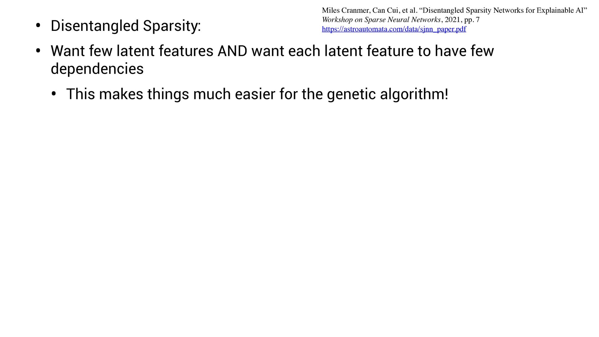
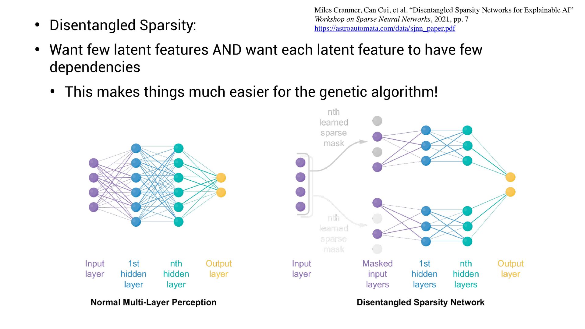
68. • Disentangled Sparsity: • Want few latent features AND want each latent feature to have few dependencies Miles Cranmer, Can Cui, et al. “Disentangled Sparsity Networks for Explainable AI” 
 Workshop on Sparse Neural Networks, 2021, pp. 7 
 https://astroautomata.com/data/sjnn_paper.pdf
69. • Disentangled Sparsity: • Want few latent features AND want each latent feature to have few dependencies • This makes things much easier for the genetic algorithm! Miles Cranmer, Can Cui, et al. “Disentangled Sparsity Networks for Explainable AI” 
 Workshop on Sparse Neural Networks, 2021, pp. 7 
 https://astroautomata.com/data/sjnn_paper.pdf
70. • Disentangled Sparsity: • Want few latent features AND want each latent feature to have few dependencies • This makes things much easier for the genetic algorithm! Miles Cranmer, Can Cui, et al. “Disentangled Sparsity Networks for Explainable AI” 
 Workshop on Sparse Neural Networks, 2021, pp. 7 
 https://astroautomata.com/data/sjnn_paper.pdf
71. Example: Graph neural network activations = forces, under a sparsity regularization Miles Cranmer, Alvaro Sanchez-Gonzalez, Peter Battaglia, Rui Xu, Kyle Cranmer, David Spergel and Shirley Ho, 
 NeurIPS, 2020
72. Example: 
 Discovering Orbital Mechanics
73. Example: 
 Discovering Orbital Mechanics Can we learn Newton’s law of gravity simply by observing the solar system?
 
 Unknown masses, and unknown dynamical model.
74. “Rediscovering orbital mechanics with machine learning” (2022) 
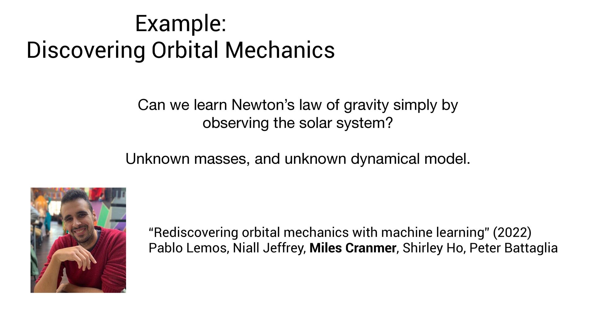
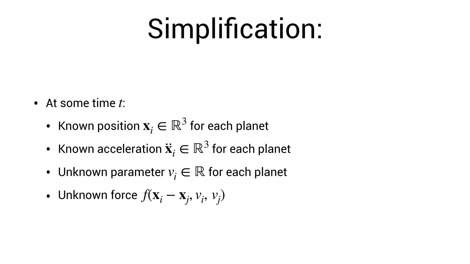
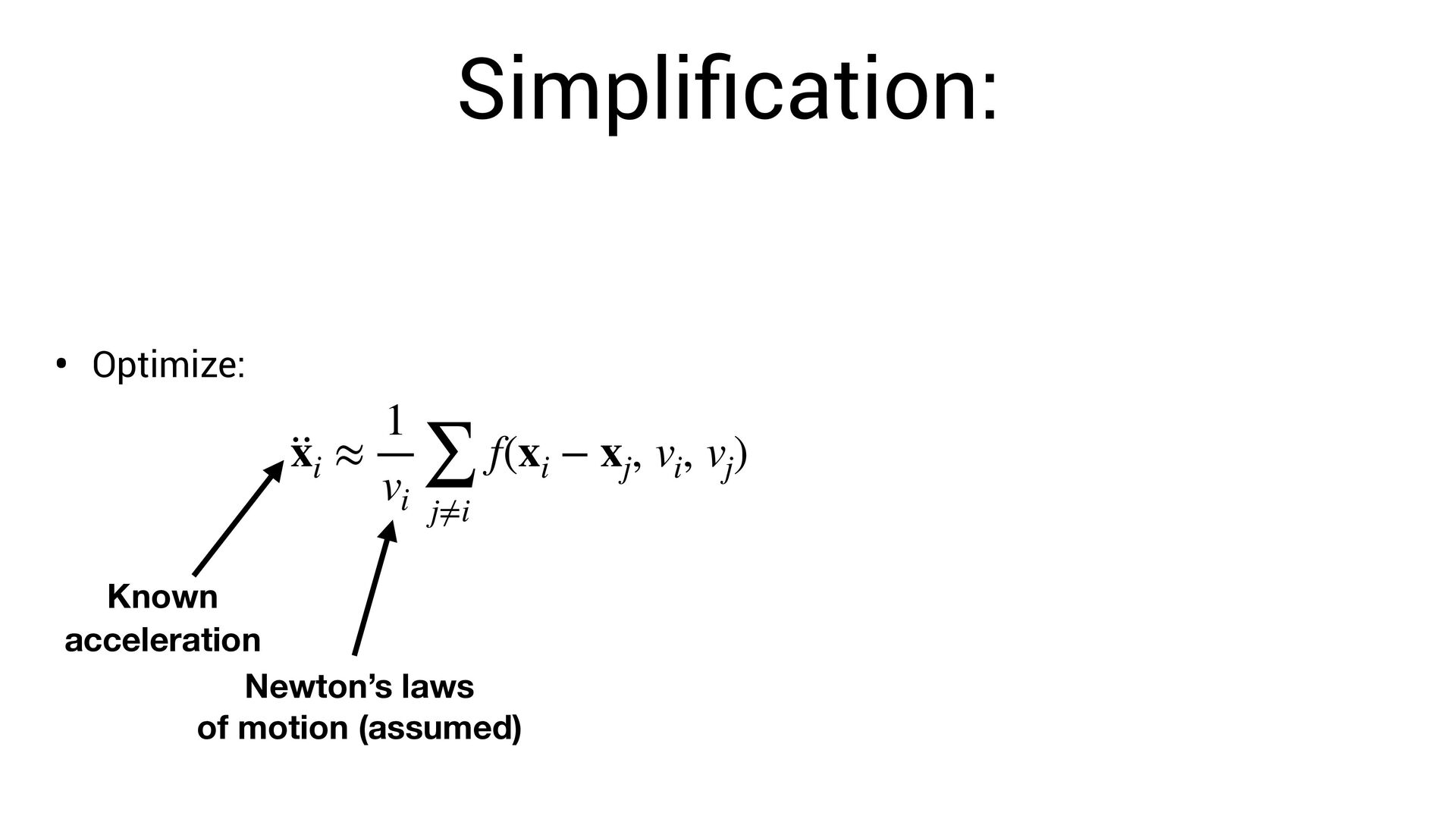
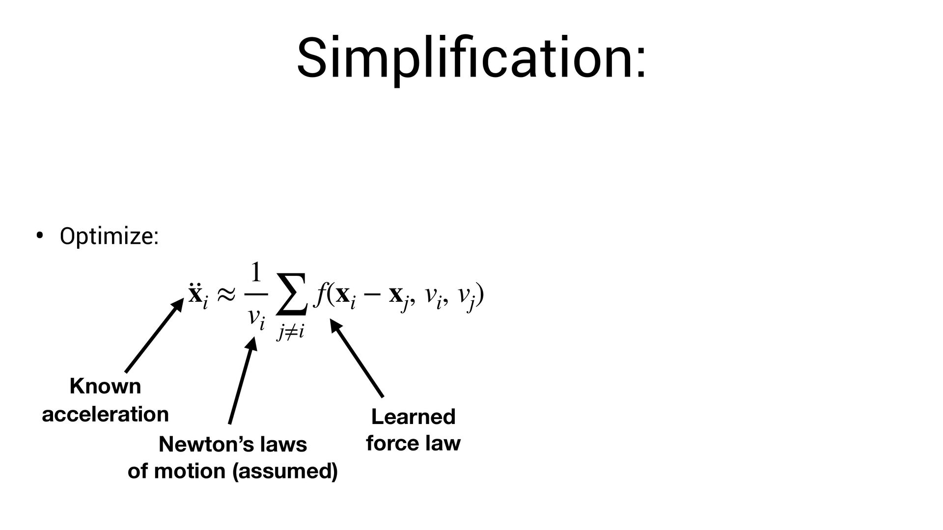
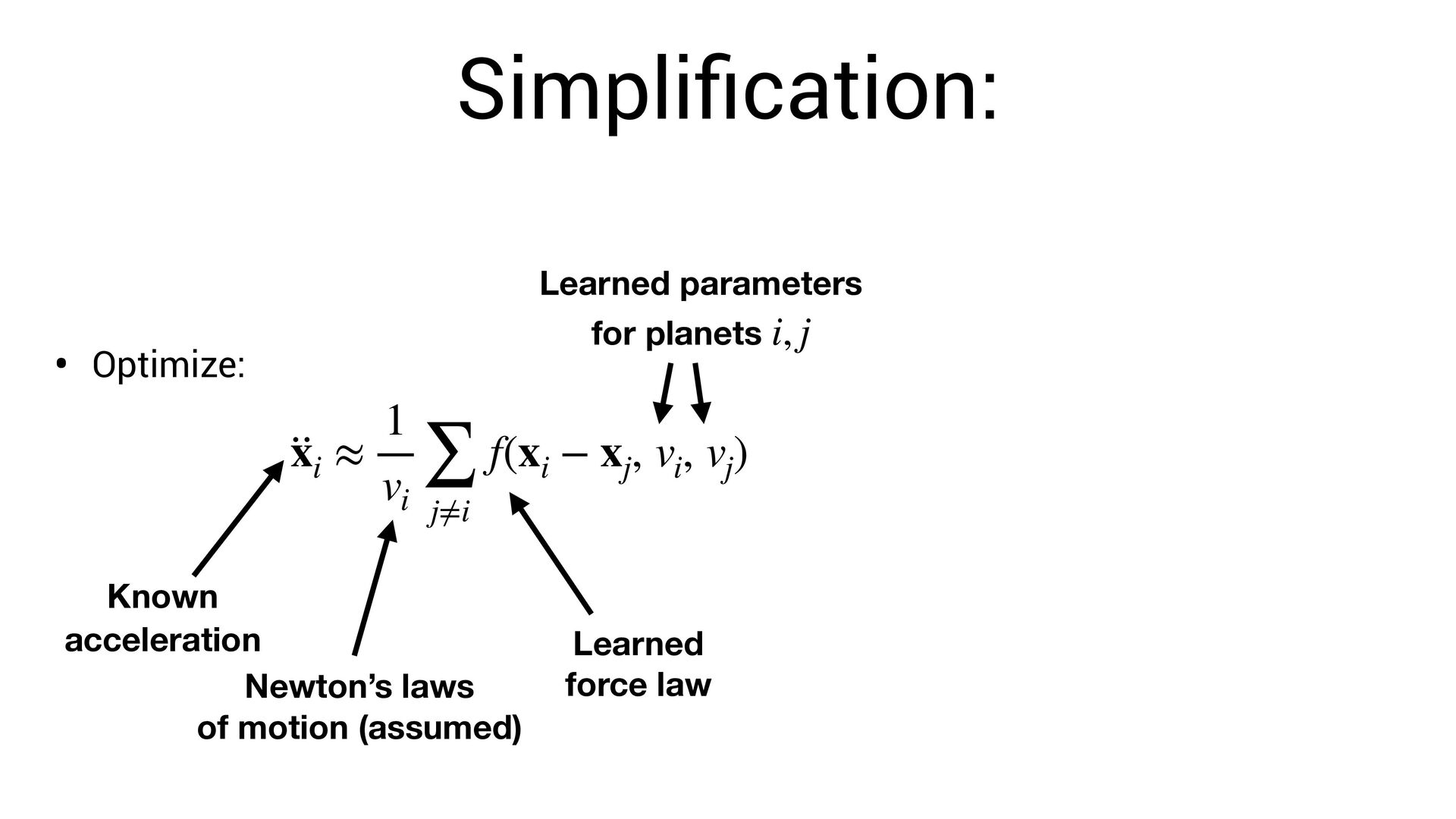
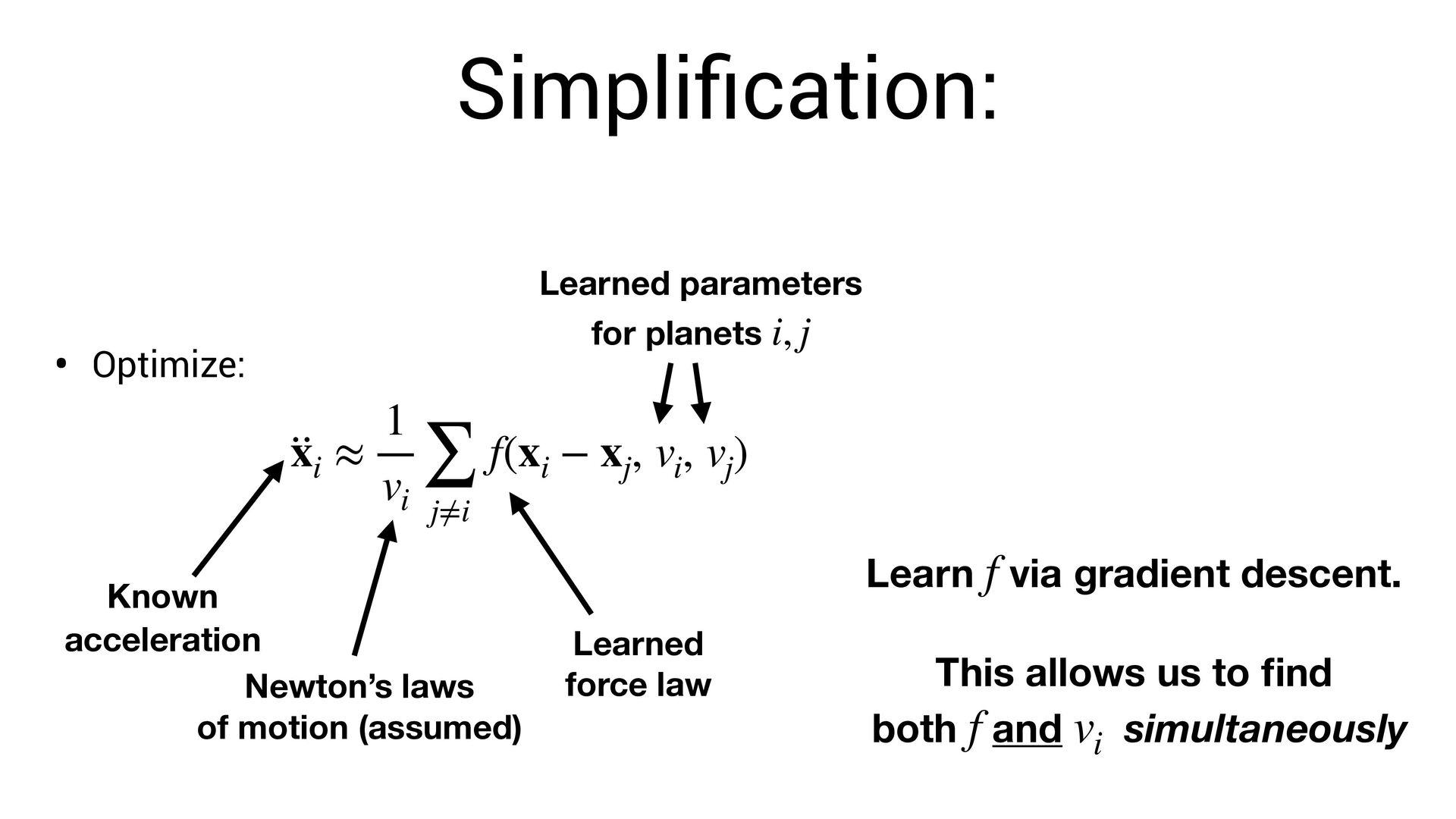
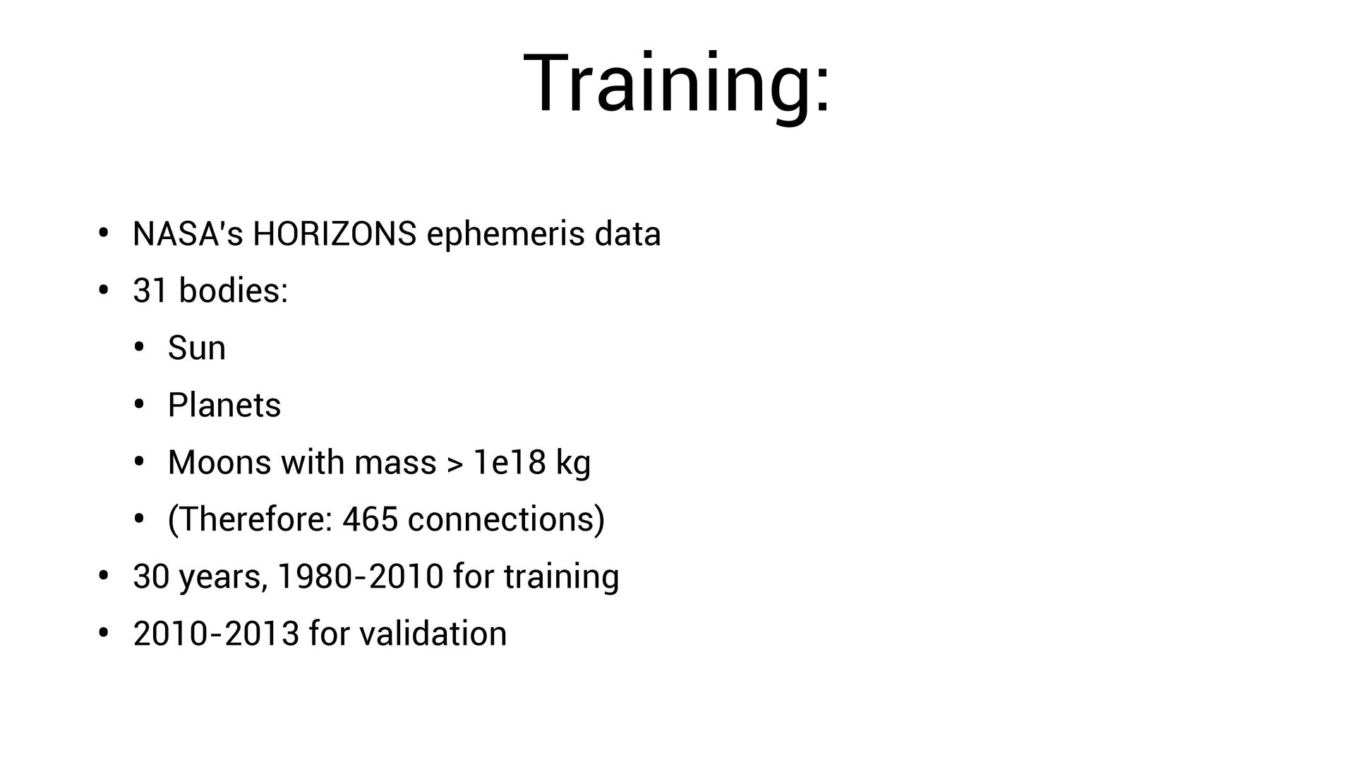
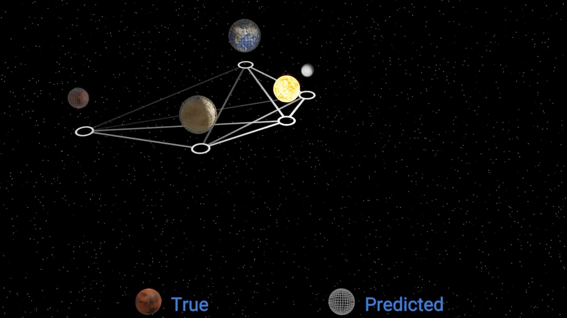
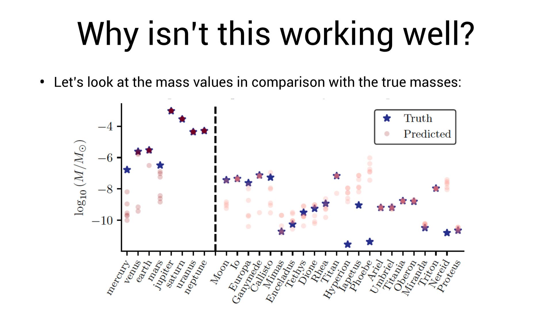
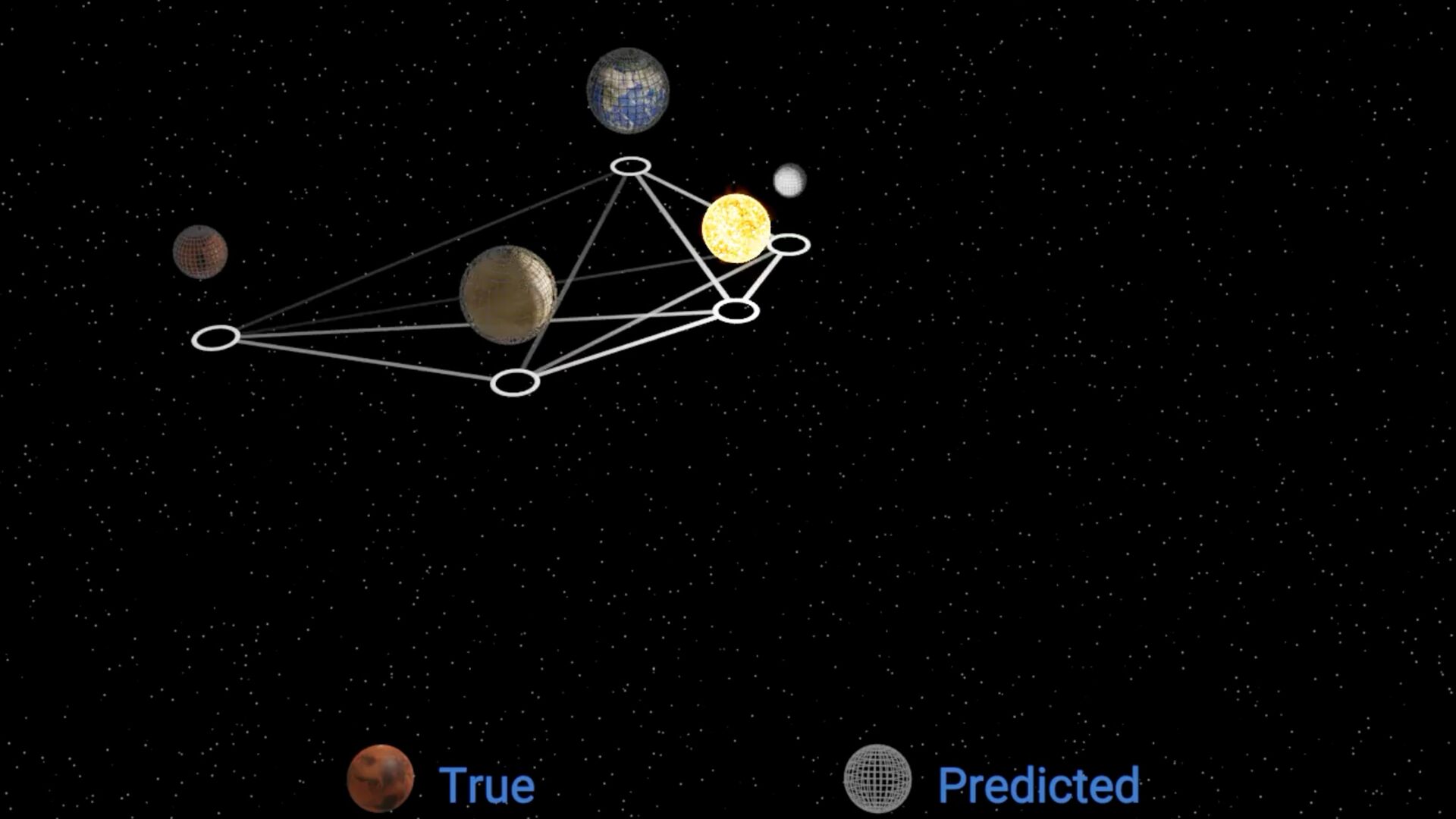
 Pablo Lemos, Niall Jeffrey, Miles Cranmer, Shirley Ho, Peter Battaglia Example: 
 Discovering Orbital Mechanics Can we learn Newton’s law of gravity simply by observing the solar system?
 
 Unknown masses, and unknown dynamical model.
75. Simpli fi cation:
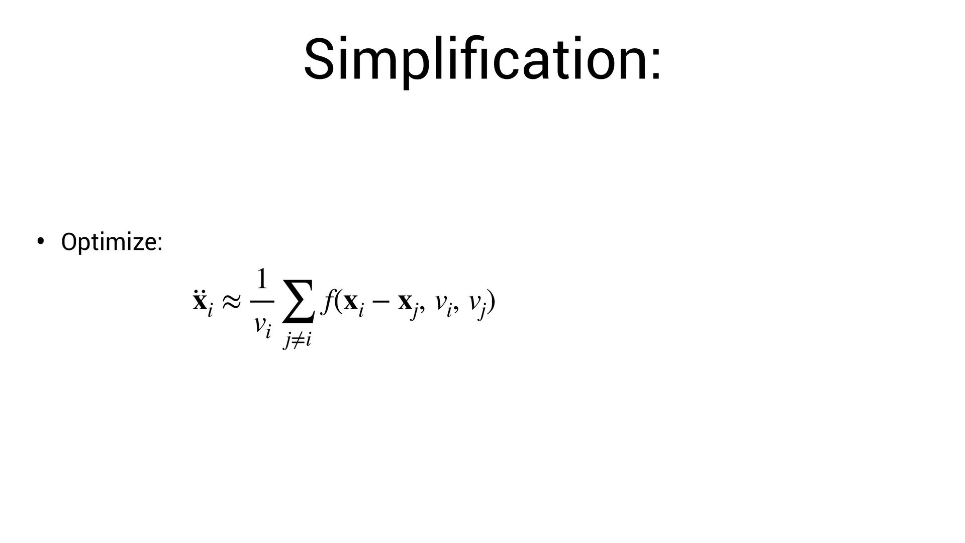
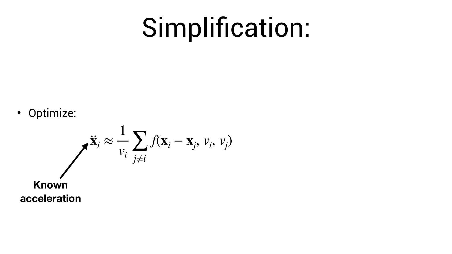
76. Simpli fi cation: • At some time : • Known position for each planet • Known acceleration for each planet • Unknown parameter for each planet • Unknown force t xi ∈ ℝ3 ·· xi ∈ ℝ3 vi ∈ ℝ f(xi − xj , vi , vj )
77. Simpli fi cation:
78. Simpli fi cation: • Optimize: ·· xi ≈ 1 vi ∑ j≠i f(xi − xj , vi , vj )
79. Simpli fi cation: • Optimize: ·· xi ≈ 1 vi ∑ j≠i f(xi − xj , vi , vj ) Known acceleration
80. Simpli fi cation: • Optimize: ·· xi ≈ 1 vi ∑ j≠i f(xi − xj , vi , vj ) Known acceleration Newton’s laws
 of motion (assumed)
81. Simpli fi cation: • Optimize: ·· xi ≈ 1 vi ∑ j≠i f(xi − xj , vi , vj ) Known acceleration Learned 
 force law Newton’s laws
 of motion (assumed)
82. Simpli fi cation: • Optimize: ·· xi ≈ 1 vi ∑ j≠i f(xi − xj , vi , vj ) Known acceleration Learned 
 force law Learned parameters for planets i, j Newton’s laws
 of motion (assumed)
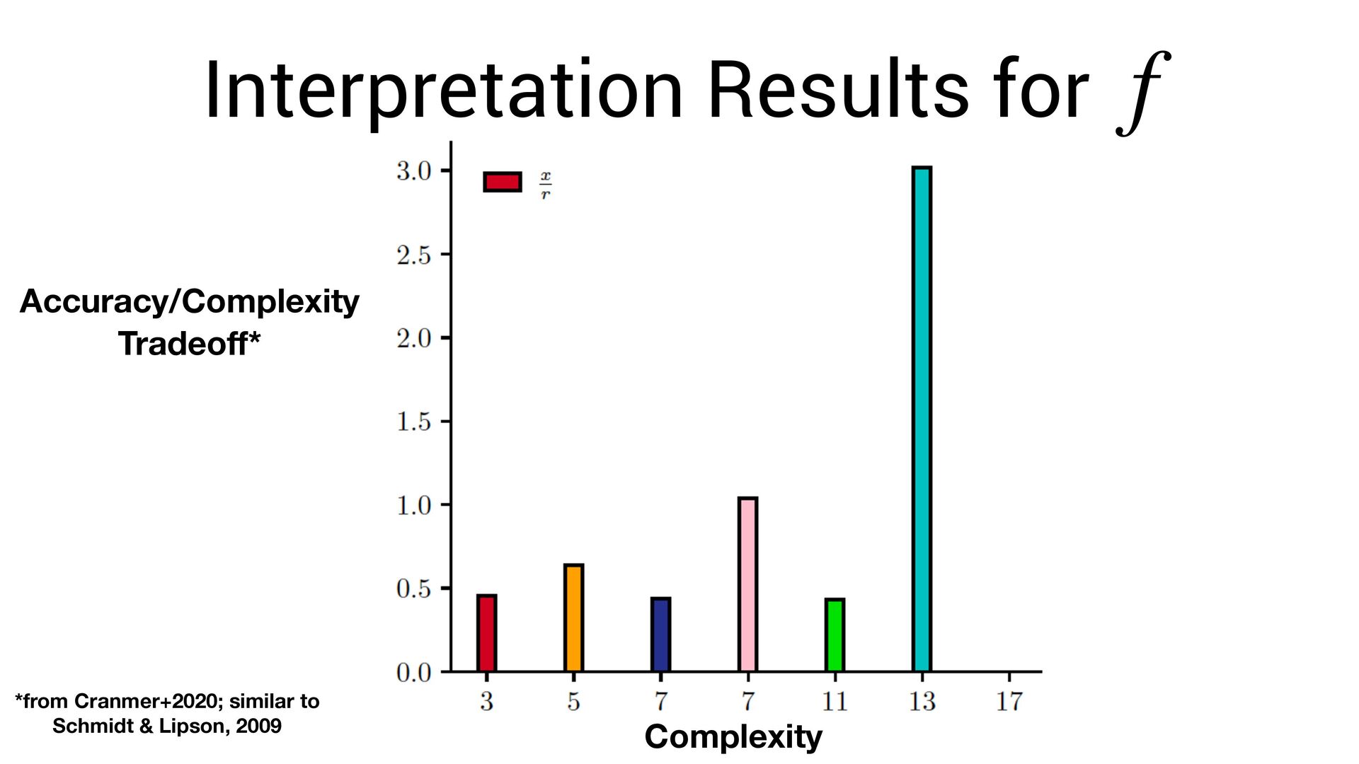
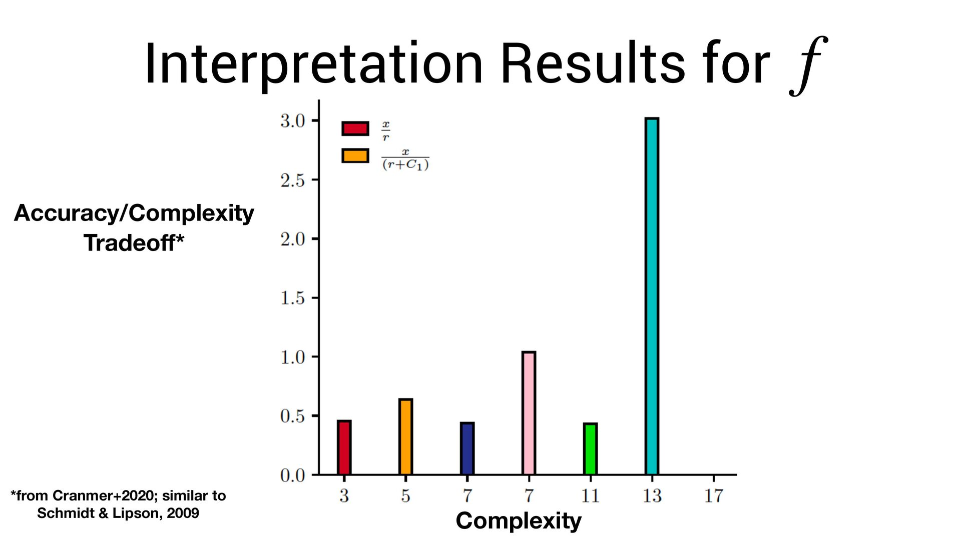
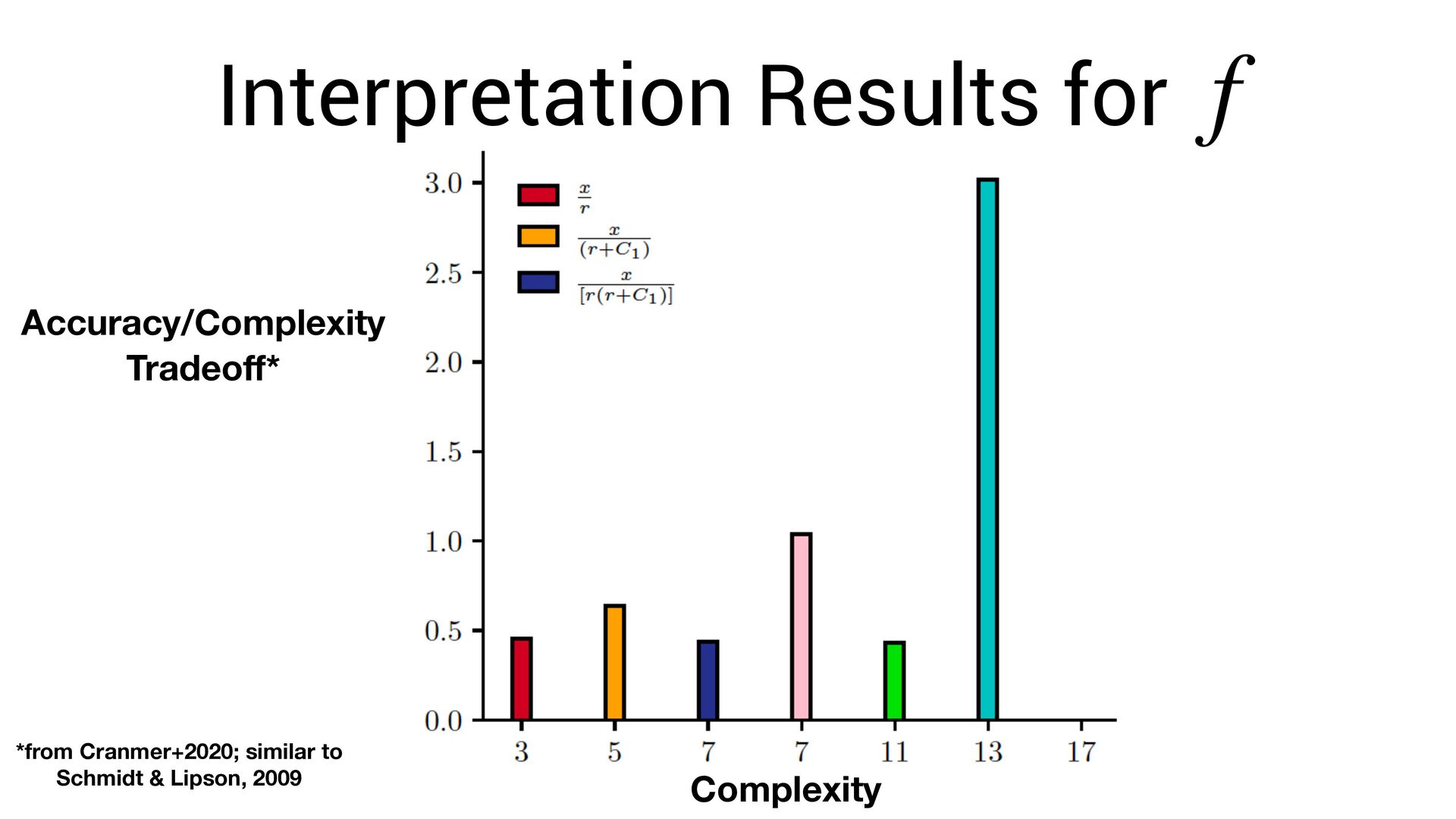
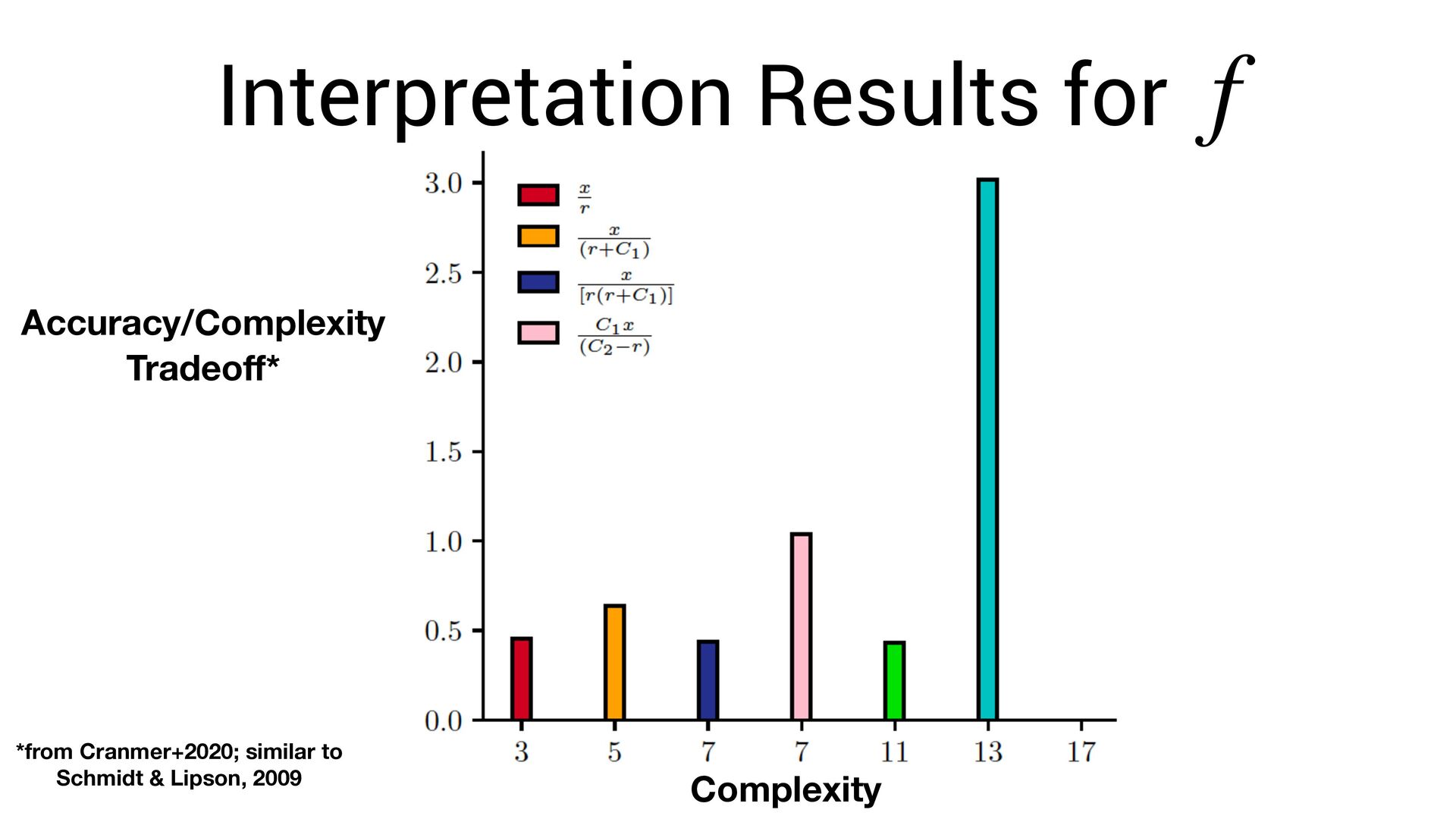
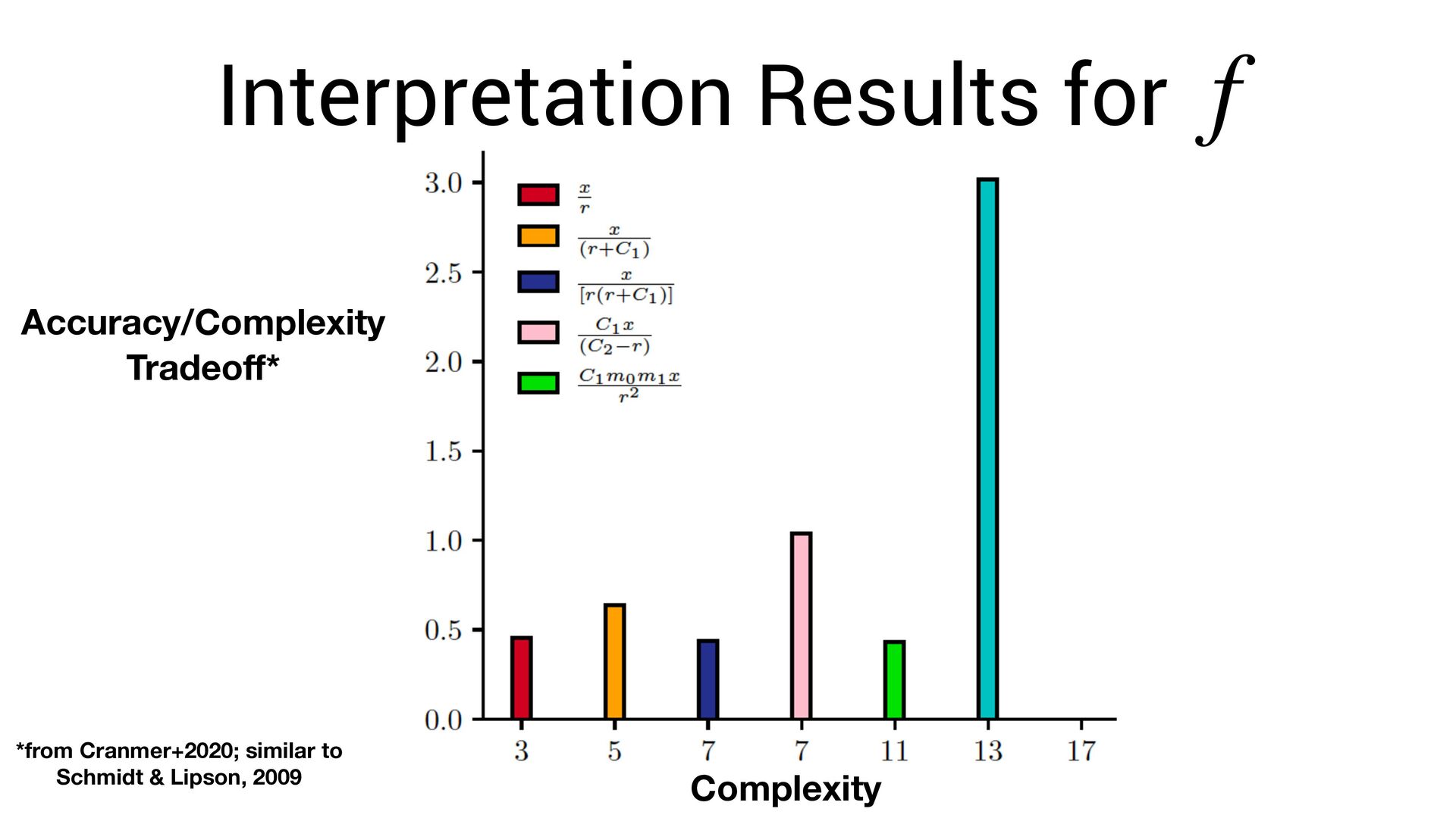
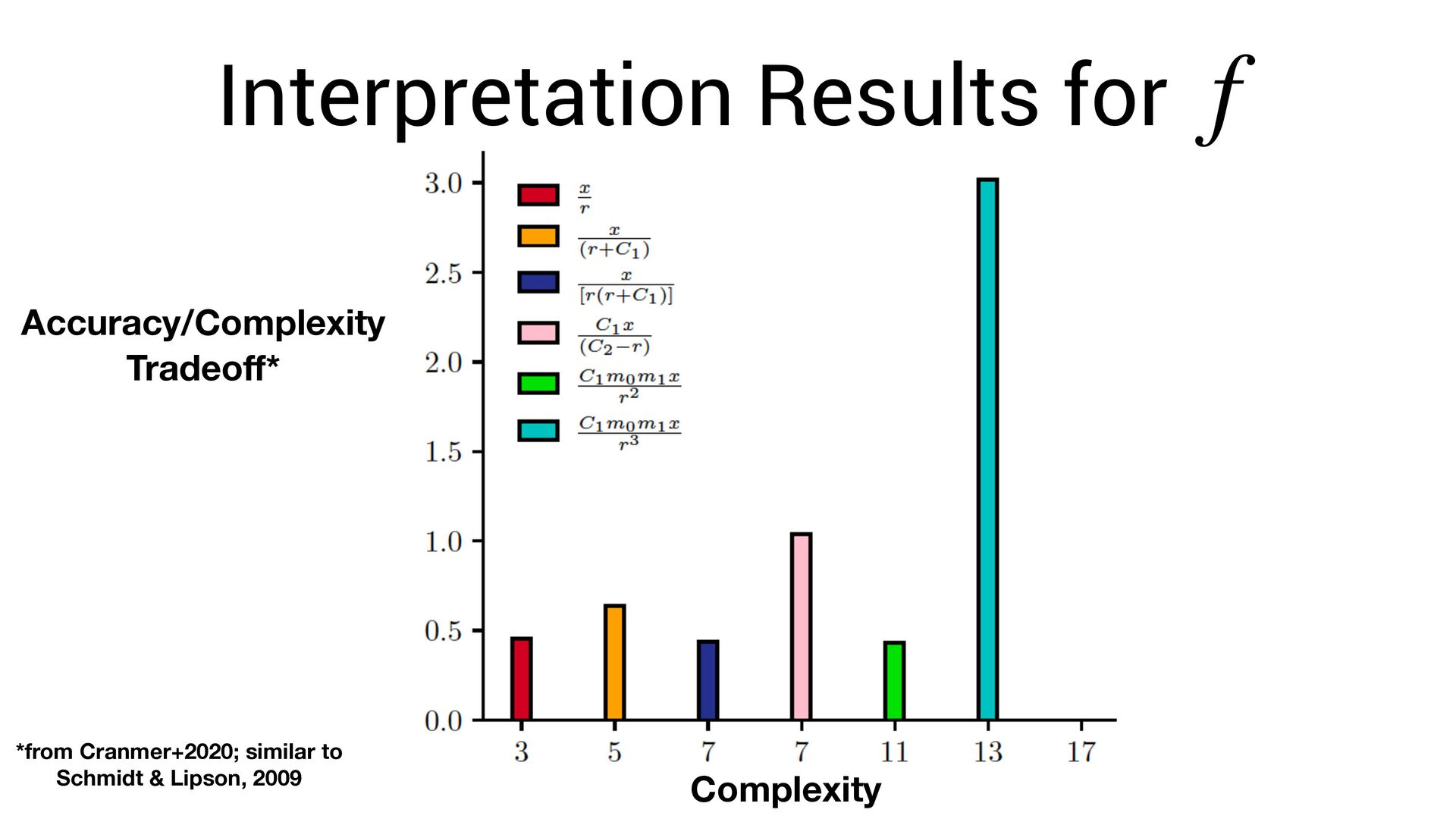
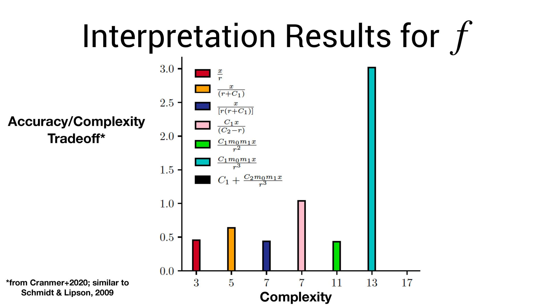
83. Simpli fi cation: • Optimize: ·· xi ≈ 1 vi ∑ j≠i f(xi − xj , vi , vj ) Known acceleration Learned 
 force law Learned parameters for planets i, j Newton’s laws
 of motion (assumed) Learn via gradient descent.
 
 This allows us to fi nd
 both and simultaneously f f vi
84. Training: • NASA’s HORIZONS ephemeris data • 31 bodies: • Sun • Planets • Moons with mass > 1e18 kg • (Therefore: 465 connections) • 30 years, 1980-2010 for training • 2010-2013 for validation
87. Next: interpretation ·· xi ≈ 1 vi ∑ j≠i f(xi − xj , vi , vj ) Approximate input/output of with symbolic regression. f
88. Interpretation Results for f Complexity Accuracy/Complexity Tradeo ff * *from Cranmer+2020; similar to Schmidt & Lipson, 2009
89. Interpretation Results for f Complexity Accuracy/Complexity Tradeo ff * *from Cranmer+2020; similar to Schmidt & Lipson, 2009
90. Interpretation Results for f Complexity Accuracy/Complexity Tradeo ff * *from Cranmer+2020; similar to Schmidt & Lipson, 2009
91. Interpretation Results for f Complexity Accuracy/Complexity Tradeo ff * *from Cranmer+2020; similar to Schmidt & Lipson, 2009
92. Interpretation Results for f Complexity Accuracy/Complexity Tradeo ff * *from Cranmer+2020; similar to Schmidt & Lipson, 2009
93. Interpretation Results for f Complexity Accuracy/Complexity Tradeo ff * *from Cranmer+2020; similar to Schmidt & Lipson, 2009
94. Interpretation Results for f Complexity Accuracy/Complexity Tradeo ff * *from Cranmer+2020; similar to Schmidt & Lipson, 2009
95. Interpretation Results for f Complexity Accuracy/Complexity Tradeo ff * *from Cranmer+2020; similar to Schmidt & Lipson, 2009 = − d(log(error)) d(complexity)
96. Test the symbolic model:
99. Why isn’t this working well? • Let’s look at the mass values in comparison with the true masses:
100. Why isn’t this working well? • Let’s look at the mass values in comparison with the true masses:
101. Solution: re-optimize ! vi
102. Solution: re-optimize ! vi • The were optimized for the neural network. vi
103. Solution: re-optimize ! vi • The were optimized for the neural network. vi • The symbolic formula is not a *perfect* approximation of the network.
104. Solution: re-optimize ! vi • The were optimized for the neural network. vi • The symbolic formula is not a *perfect* approximation of the network. • Thus: we need to re-optimize for the symbolic function ! vi f
108. V. Ongoing Work: Turbulence Work includes: Dmitrii Kochkov, Keaton Burns, Drummond Fielding, and others
109. Learned Coarse Models for Ef fi cient Turbulence Simulation 
 (ICLR 2022) 
 
 Kimberly Stachenfeld, Drummond B. Fielding, Dmitrii Kochkov, Miles Cranmer, 
 Tobias Pfaff, Jonathan Godwin, Can Cui, Shirley Ho, Peter Battaglia, Alvaro Sanchez- Gonzalez Example:
110. Learned Coarse Models for Ef fi cient Turbulence Simulation 
 (ICLR 2022) 
 
 Kimberly Stachenfeld, Drummond B. Fielding, Dmitrii Kochkov, Miles Cranmer, 
 Tobias Pfaff, Jonathan Godwin, Can Cui, Shirley Ho, Peter Battaglia, Alvaro Sanchez- Gonzalez Example: Trained to reproduce turbulence simulations at lower resolution:
111. Learned Coarse Models for Ef fi cient Turbulence Simulation 
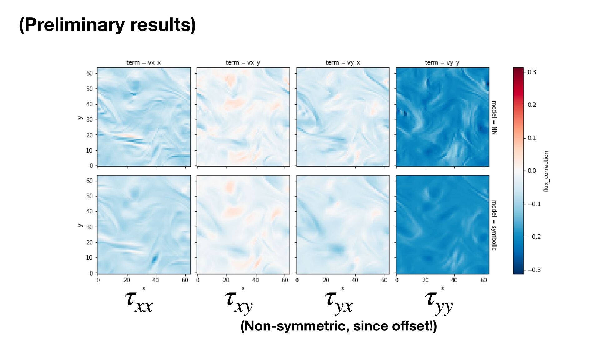
 (ICLR 2022) 
 
 Kimberly Stachenfeld, Drummond B. Fielding, Dmitrii Kochkov, Miles Cranmer, 
 Tobias Pfaff, Jonathan Godwin, Can Cui, Shirley Ho, Peter Battaglia, Alvaro Sanchez- Gonzalez 1000x speedup: Example: Trained to reproduce turbulence simulations at lower resolution:
112. Learned Coarse Models for Ef fi cient Turbulence Simulation 
 (ICLR 2022) 
 
 Kimberly Stachenfeld, Drummond B. Fielding, Dmitrii Kochkov, Miles Cranmer, 
 Tobias Pfaff, Jonathan Godwin, Can Cui, Shirley Ho, Peter Battaglia, Alvaro Sanchez- Gonzalez 1000x speedup: How did the model actually achieve this? Example: Trained to reproduce turbulence simulations at lower resolution:
113. (Preliminary results) τxx τxy τyx τyy (Non-symmetric, since o ff set!)
114. Summary • Symbolic distillation is a technique for translating ML models into a domain speci fi c language • Can do this for expressions/programs using PySR • Exciting future applications in understanding turbulence, and other physical systems