Nullspace MPC

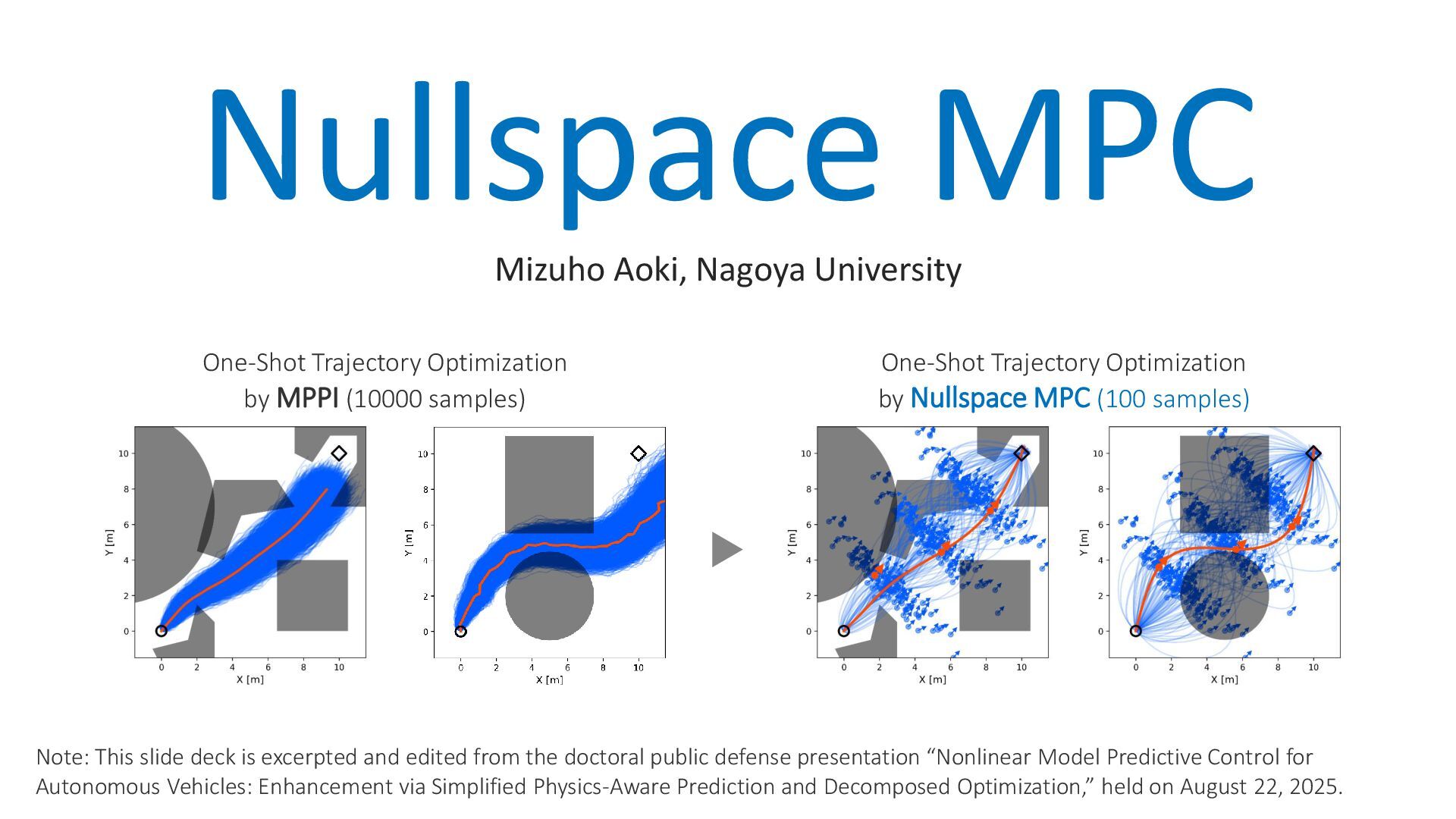
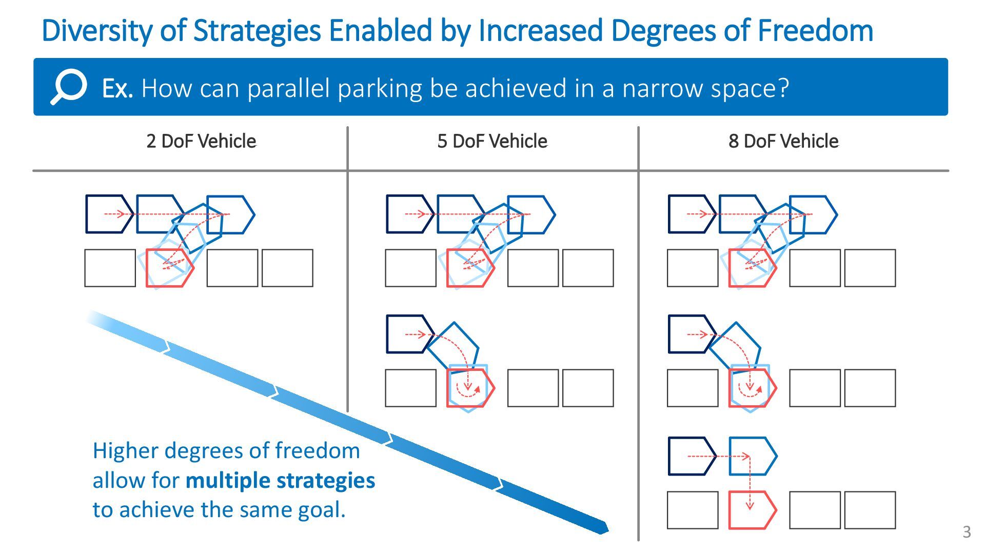
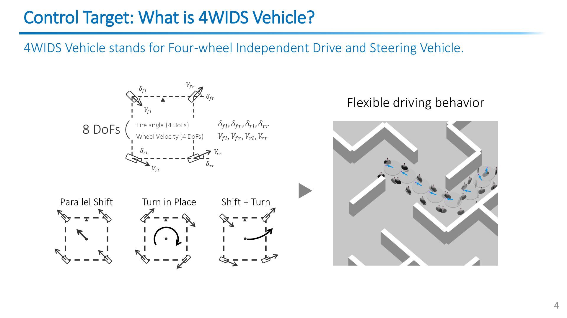
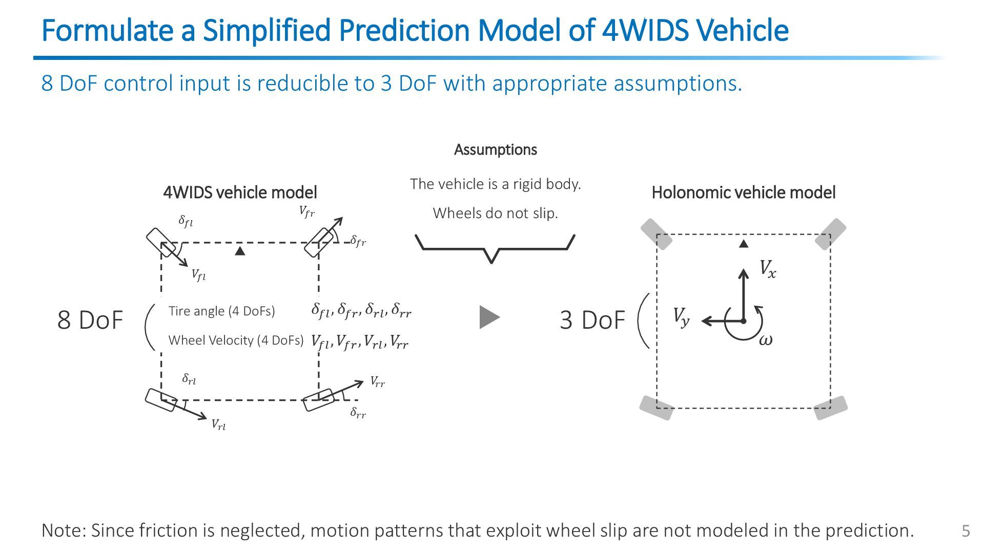
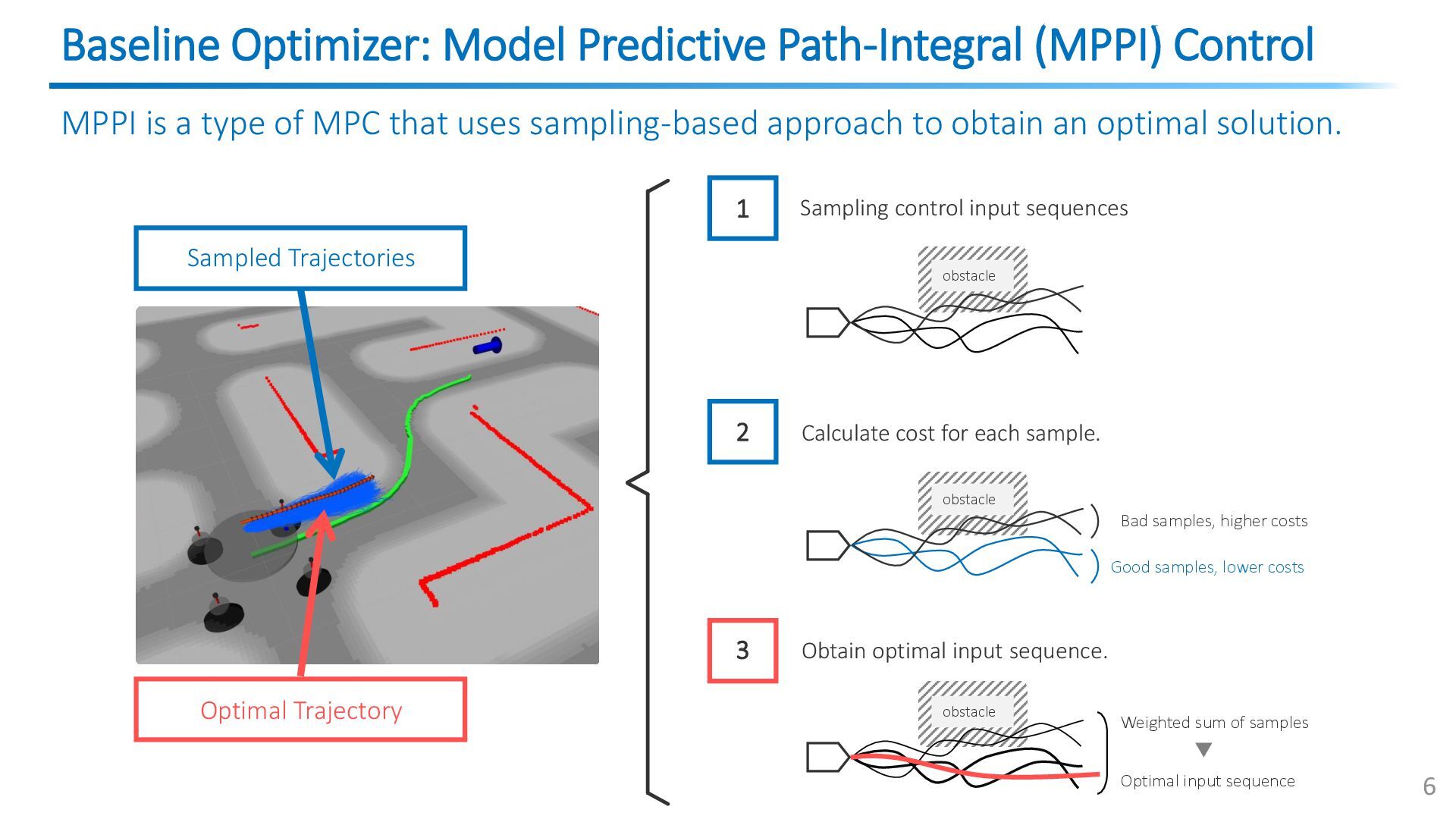
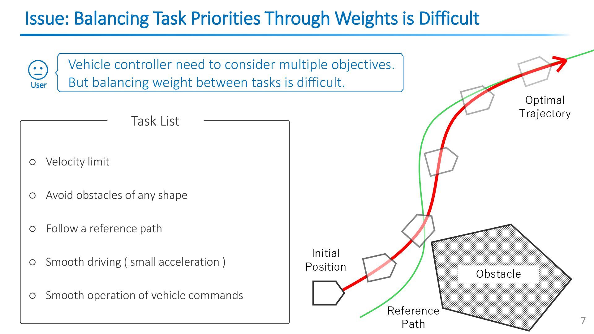
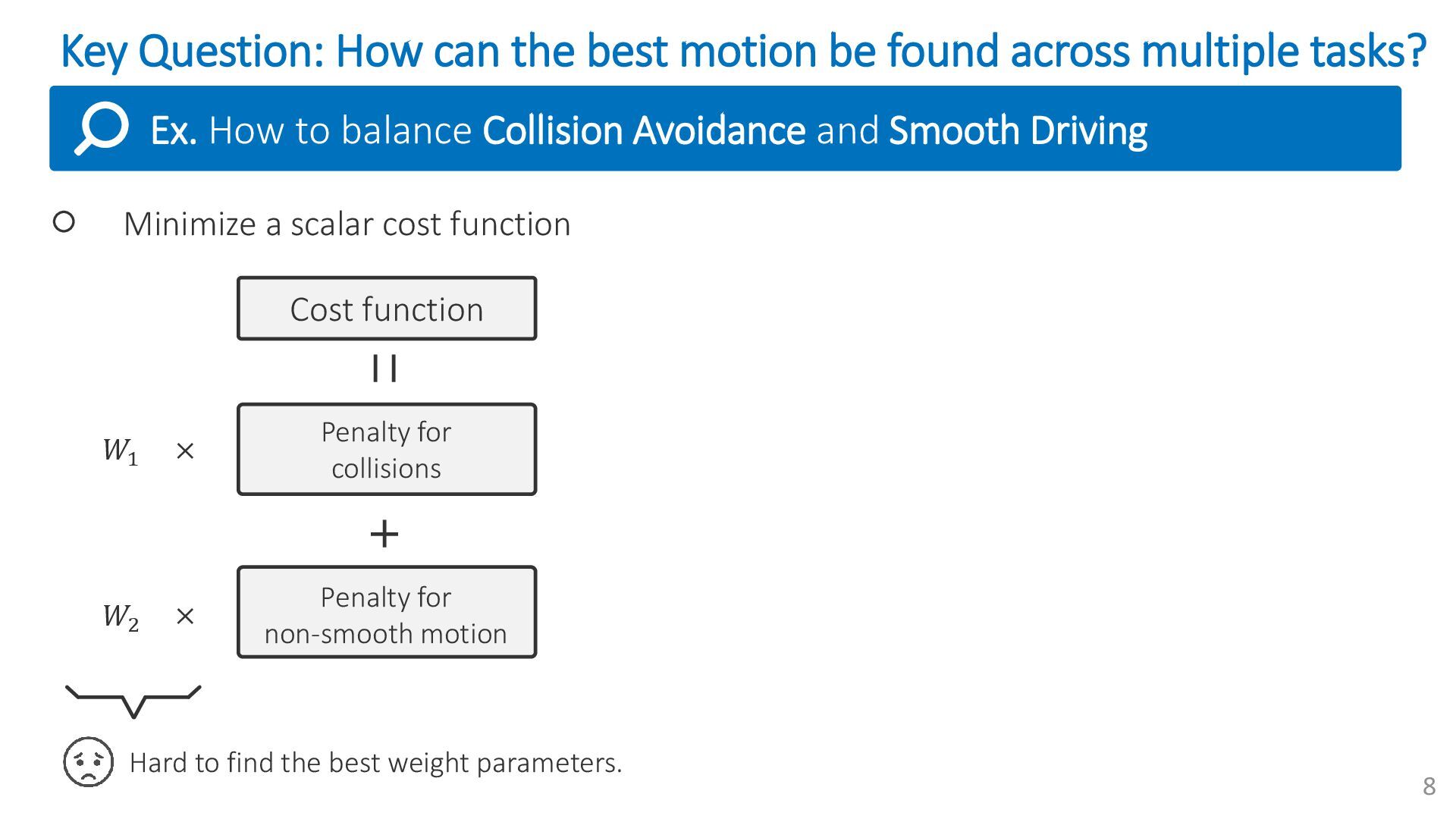
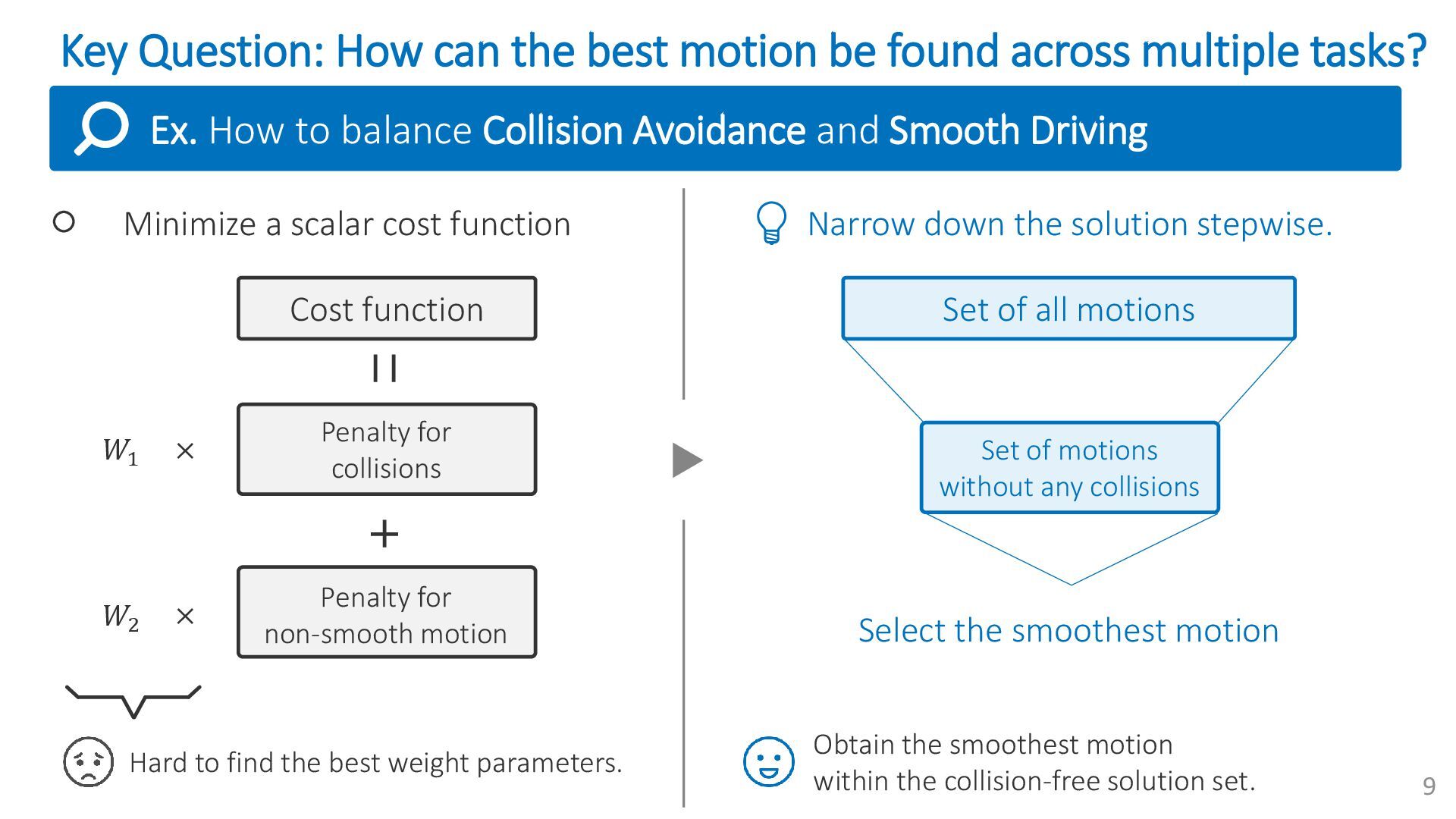
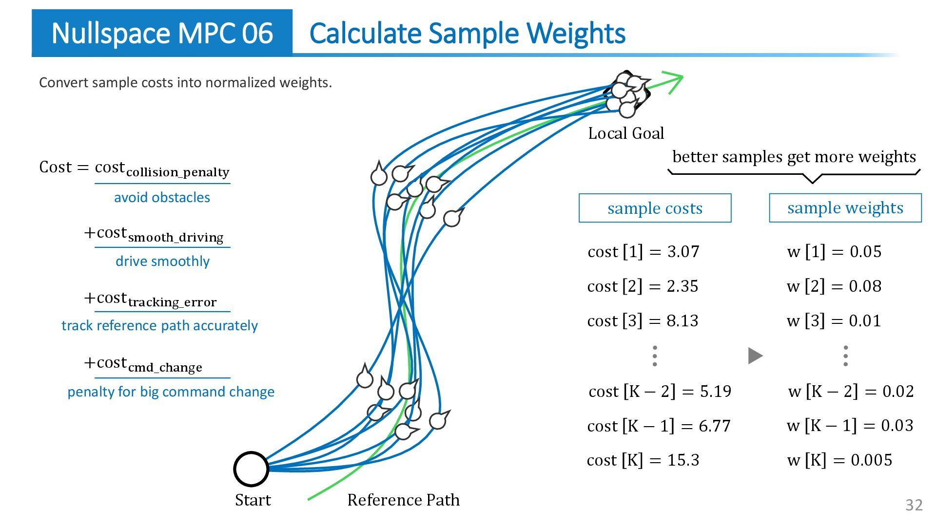
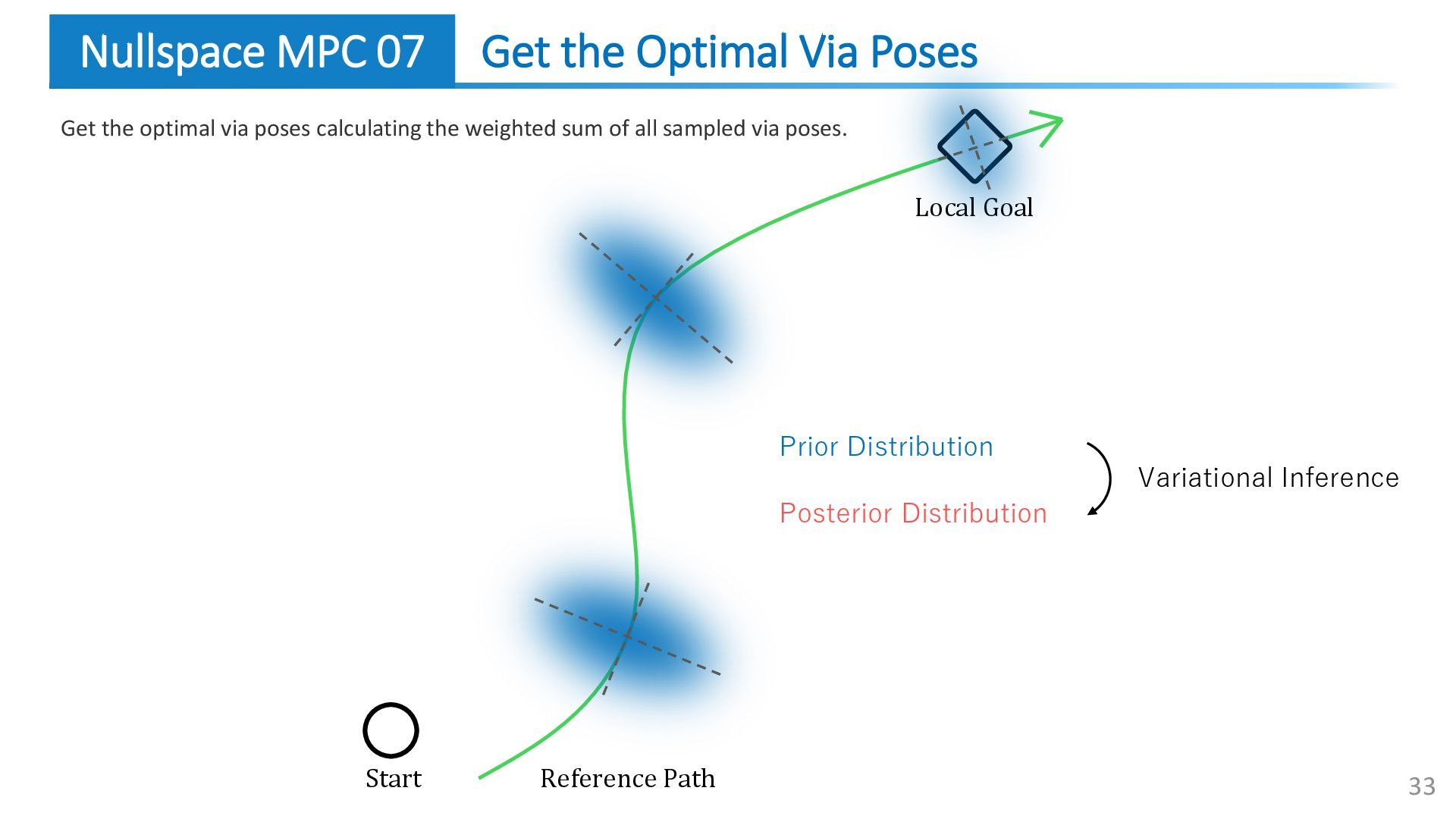
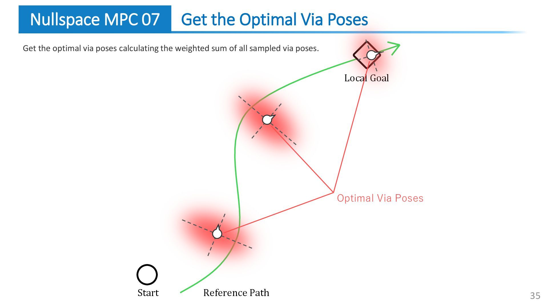
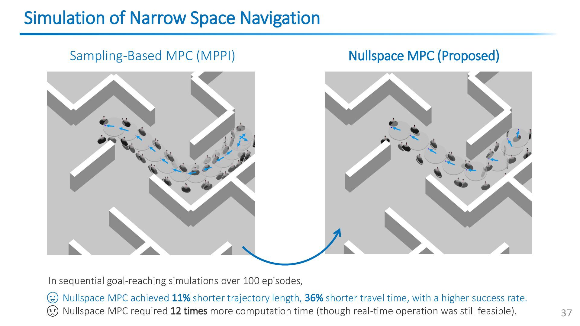
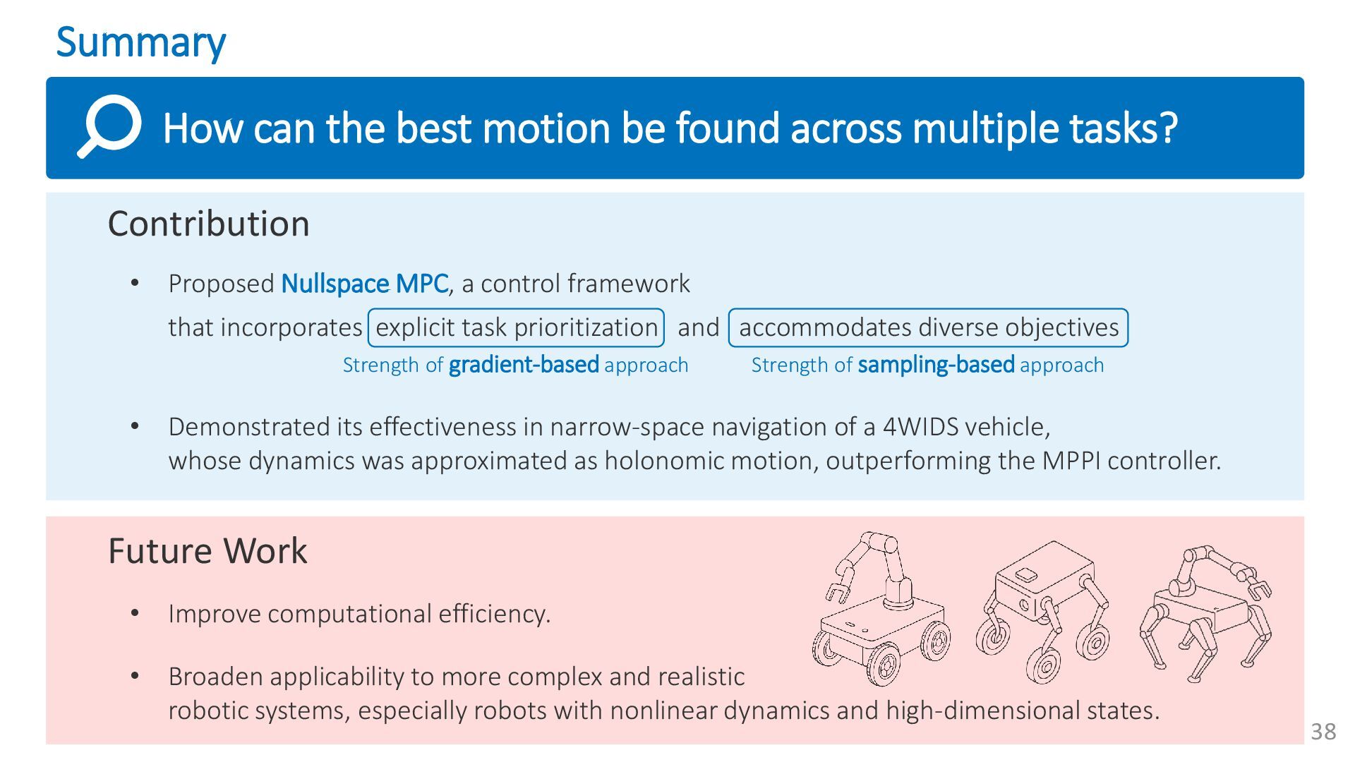
Explanation of Nullspace MPC, a novel control framework that incorporates explicit task prioritization and accommodates diverse objectives. Demonstrated its effectiveness in narrow-space navigation of a swerve drive robot.

Project website: mizuhoaoki.github.io/projects/nullspace_mpc
Open-source code: github.com/MizuhoAOKI/nullspace_mpc

Transcript

1. Nullspace MPC Note: This slide deck is excerpted and edited from the doctoral public defense presentation “Nonlinear Model Predictive Control for Autonomous Vehicles: Enhancement via Simplified Physics-Aware Prediction and Decomposed Optimization,” held on August 22, 2025. One-Shot Trajectory Optimization by MPPI (10000 samples) One-Shot Trajectory Optimization by Nullspace MPC (100 samples) Mizuho Aoki, Nagoya University
2. Background: Diversifying Mobility Designs 2 Reference [1] https://lexus.jp/models/?padid=from_not_ljptop_footer_carlineup [2] https://www.youtube.com/watch?v=QC6Q4Fge3uE [3] https://response.jp/article/2014/12/12/239488.html [4] https://www.youtube.com/watch?v=Bbw_smfOgVA [4] [2] [3] Mobilities with different degrees of freedom (DoF) are appearing. [1] 2 DoF 5 DoF 8 DoF 8 DoF Positive Aspects Negative Aspects Higher mobility performance will be beneficial. Capable of meeting a wide variety of user needs. Difficult to exploit performance of each vehicle. Keeping safety must be ensured for any vehicle. Consider the challenge of adding Autonomous Driving ability in these vehicles.
3. Diversity of Strategies Enabled by Increased Degrees of Freedom 3 2 DoF Vehicle 5 DoF Vehicle 8 DoF Vehicle Ex. How can parallel parking be achieved in a narrow space? Higher degrees of freedom allow for multiple strategies to achieve the same goal.
4. Control Target: What is 4WIDS Vehicle? 4 4WIDS Vehicle stands for Four-wheel Independent Drive and Steering Vehicle. Flexible driving behavior 𝛿𝑓𝑟 𝛿𝑟𝑟 𝛿𝑟𝑙 𝛿𝑓𝑙 𝑉𝑟𝑙 𝑉 𝑟𝑟 𝑉𝑓𝑟 𝑉𝑓𝑙 Tire angle (4 DoFs) 𝛿𝑓𝑙 , 𝛿𝑓𝑟 , 𝛿𝑟𝑙 , 𝛿𝑟𝑟 Wheel Velocity (4 DoFs) 𝑉𝑓𝑙 , 𝑉𝑓𝑟 , 𝑉𝑟𝑙 , 𝑉 𝑟𝑟 8 DoFs Parallel Shift Turn in Place Shift + Turn
5. Formulate a Simplified Prediction Model of 4WIDS Vehicle 5 8 DoF control input is reducible to 3 DoF with appropriate assumptions. 𝛿𝑓𝑟 𝛿𝑟𝑟 𝛿𝑟𝑙 𝛿𝑓𝑙 𝑉𝑟𝑙 𝑉 𝑟𝑟 𝑉𝑓𝑟 𝑉𝑓𝑙 Tire angle (4 DoFs) 𝛿𝑓𝑙 , 𝛿𝑓𝑟 , 𝛿𝑟𝑙 , 𝛿𝑟𝑟 Wheel Velocity (4 DoFs) 𝑉𝑓𝑙 , 𝑉𝑓𝑟 , 𝑉𝑟𝑙 , 𝑉 𝑟𝑟 8 DoF 𝑉 𝑥 𝑉 𝑦 𝜔 3 DoF The vehicle is a rigid body. Wheels do not slip. Assumptions Holonomic vehicle model 4WIDS vehicle model Note: Since friction is neglected, motion patterns that exploit wheel slip are not modeled in the prediction.
6. Baseline Optimizer: Model Predictive Path-Integral (MPPI) Control 6 Sampled Trajectories Optimal Trajectory 1 2 3 Sampling control input sequences Calculate cost for each sample. Obtain optimal input sequence. Bad samples, higher costs Good samples, lower costs Weighted sum of samples Optimal input sequence obstacle obstacle obstacle MPPI is a type of MPC that uses sampling-based approach to obtain an optimal solution.
7. Issue: Balancing Task Priorities Through Weights is Difficult 7 Vehicle controller need to consider multiple objectives. But balancing weight between tasks is difficult. User Initial Position Reference Path ◦ Velocity limit ◦ Avoid obstacles of any shape ◦ Follow a reference path ◦ Smooth driving ( small acceleration ) ◦ Smooth operation of vehicle commands Task List Obstacle Optimal Trajectory
8. Ex. How to balance Collision Avoidance and Smooth Driving Minimize a scalar cost function Penalty for collisions Cost function Penalty for non-smooth motion 𝑊1 𝑊2 × × Hard to find the best weight parameters. 8 Key Question: How can the best motion be found across multiple tasks?
9. Ex. How to balance Collision Avoidance and Smooth Driving Minimize a scalar cost function Penalty for collisions Cost function Penalty for non-smooth motion 𝑊1 𝑊2 × × Hard to find the best weight parameters. Narrow down the solution stepwise. Set of all motions Set of motions without any collisions Select the smoothest motion Obtain the smoothest motion within the collision-free solution set. 9 Key Question: How can the best motion be found across multiple tasks?
10. 10 𝒮𝒯 𝑖 𝒮𝒯 𝑗 𝒮𝒯 𝑗 𝒮𝒯 𝑖 𝒮𝒯 𝑖 ∩ > 𝒮𝒯 𝑗 Introducing a Priority-Aware Operator ∩ to Narrow Down a Solution Set • Let 𝒙 be a solution vector of a motion planning problem. > • 𝓢𝓣𝒊 is a solution set of 𝒙 satisfying Task 𝓣𝒊 , 𝓢𝓣𝒋 is a solution set of 𝒙 satisfying Task 𝓣𝒋 • Now Task 𝓣𝒊 has higher priority than Task 𝓣𝒋 , obtain an intersection set between them considering the task priority with a new operator . 𝒮𝒯 𝑖 ∩ > 𝒮𝒯 𝑗 is defined as follows. 𝒮𝒯 𝑖 ∩𝒮𝒯 𝑗 ≠ 𝜙 (𝑎) 𝑖𝑓 𝒮𝒯 𝑖 ∩𝒮𝒯 𝑗 = 𝜙 (𝑏) 𝑖𝑓 ∩ > Here, (Closest satisfying 𝓣𝒊 ) 𝒮𝒯 𝑖 ∩ > 𝒮𝒯 𝑗 (= 𝒮𝒯 𝑖 ∩ 𝒮𝒯 𝑗 )
11. Hierarchical Prioritization Framework Only for Linear Tasks 11 Question Key Idea Task: ቊ 𝐀𝒙 = 𝒃 𝐃𝒙 ≤ 𝒇 Definition Linear Equality Linear Inequality Task is a set of conditions that solution 𝒙 tries to satisfy. Move solution 𝒙 to achieve a target task while keeping higher-level tasks satisfied. Task 1 > Task 2 > … > Task N High Priority Low Priority List of values to be found How can multiple tasks be achieved considering priorities?
12. Hierarchical Prioritization Framework Only for Linear Tasks 12 Question Key Idea Task: ቊ 𝐀𝒙 = 𝒃 𝐃𝒙 ≤ 𝒇 Definition Linear Equality Linear Inequality Task is a set of conditions that solution 𝒙 tries to satisfy. Move solution 𝒙 to achieve a target task while keeping higher-level tasks satisfied. Task 1 > Task 2 > … > Task N High Priority Low Priority Apply Task 1 𝒙∗ : tentative optimal solution All solution set for 𝒙 𝐀1 𝒙 = 𝒃1 , 𝐃1 𝒙 ≤ 𝒇1 Apply Task 2 𝐀2 𝒙 = 𝒃2 , 𝐃2 𝒙 ≤ 𝒇2 Apply Task 3 𝐀3 𝒙 = 𝒃3 , 𝐃3 𝒙 ≤ 𝒇3 This 𝒙∗ follows Task 1 > Task 2 > Task 3 priority. 2 1 3 2 1 1 List of values to be found How can multiple tasks be achieved considering priorities?
13. Mathematical Tools for Prioritization 13 Linear Inequality Linear Equality 𝐀𝒙 = 𝒃 𝐃𝒙 ≤ 𝒇 𝒙2 = 𝒙1 + 𝓝 𝐀1 𝒛 , 𝐀1 𝒙1 = 𝒃1 . 𝐀1 𝓝 𝐀1 = 𝟎 . Let 𝒙1 be a vector which satisfies a linear equality, Here 𝓝 𝐀1 is a nullspace basis matrix of 𝐀1 , Then 𝒙2 below always satisfies 𝐀1 𝒙2 = 𝒃1 𝐀1 𝒙2 = 𝐀1 𝒙1 + 𝓝 𝐀1 𝑧 , = 𝐀1 𝒙1 + 𝐀1 𝓝 𝐀1 𝑧, = 𝐀1 𝒙1 + 𝟎 = 𝒃1 . arbitrary vector minimize 𝒗𝟐 𝒗𝟐 2 ∵ 𝐃𝟏 𝒙 − 𝒇𝟏 ≤ 𝟎 𝐃𝟐 𝒙 − 𝒇𝟐 ≤ 𝒗𝟐 𝒔. 𝒕. Try to satisfy 𝐃𝟐 𝒙 ≤ 𝒇𝟐 while keeping 𝐃𝟏 𝒙 ≤ 𝒇𝟏 High Priority Low Priority Low Priority High Priority 𝐃𝟏 𝒙 ≤ 𝒇𝟏 𝒗𝟐 = 𝟎 𝐃𝟐 𝒙 ≤ 𝒇𝟐 𝐃𝟏 𝒙 ≤ 𝒇𝟏 𝒗𝟐 ≠ 𝟎 𝐃𝟐 𝒙 − 𝒇𝟐 ≤ 𝒗𝟐
14. Formulate Optimization Problem for Task p+1 14 Update tentative solution 𝒙∗ to satisfy Task p+1 ( 𝐀𝑝+1 𝒙∗ = 𝒃𝑝+1 and 𝐃𝒑+𝟏 𝒙 ≤ 𝒇𝒑+𝟏 ) without disrupting the higher-level tasks (Task 1 > … > Task p) nullspace basis matrix of all from 𝐀1 to 𝐀p 𝒙∗ is a solution considering Task 1 > … > p 𝒙∗ + 𝐙𝑝 𝑧𝑝+1 is the updated solution considering Task 1 ~ p+1
15. Priority-Based Trajectory Optimization 15 Just stopping at the start point 𝒙 = 𝑝𝑥 0, 𝑝𝑦 0, 𝜃0, 𝑣𝑥 0, 𝑣𝑦 0, 𝜔0, … , 𝑝𝑥 𝑇−1, 𝑝𝑦 𝑇−1, 𝜃𝑇−1, 𝑣𝑥 𝑇−1, 𝑣𝑦 𝑇−1, 𝜔𝑇−1, 𝑝𝑥 𝑇, 𝑝𝑦 𝑇, 𝜃𝑇 𝑇 Time series states for T steps: Find position velocity Set the initial pose at 0 step Follow the state update rules Limit velocity for all steps 𝐀1 𝒙 = 𝒃1 𝑫1 𝒙 ≤ 𝒇1 Task 1 start 𝒮𝒯 1 𝒙∗ ∈ 𝒯 1 𝒮𝒯 1 𝒮 𝒙 ∈ 𝒮, Apply 𝒙∗
16. Priority-Based Trajectory Optimization 16 Just stopping at the start point Passing through the via pose and reaching the goal 𝒙 = 𝑝𝑥 0, 𝑝𝑦 0, 𝜃0, 𝑣𝑥 0, 𝑣𝑦 0, 𝜔0, … , 𝑝𝑥 𝑇−1, 𝑝𝑦 𝑇−1, 𝜃𝑇−1, 𝑣𝑥 𝑇−1, 𝑣𝑦 𝑇−1, 𝜔𝑇−1, 𝑝𝑥 𝑇, 𝑝𝑦 𝑇, 𝜃𝑇 𝑇 Time series states for T steps: Find position velocity Set the initial pose at 0 step Follow the state update rules Limit velocity for all steps 𝐀1 𝒙 = 𝒃1 𝑫1 𝒙 ≤ 𝒇1 Pass through a via pose at Tmid step Reach to a goal pose at T step None 𝐀2 𝒙 = 𝒃2 𝑫2 𝒙 ≤ 𝒇2 Task 1 Task 2 start goal via pose start 𝒮𝒯 1 ∩ > 𝒮𝒯 2 𝒮𝒯 1 𝒙∗ ∈ 𝒙∗ ∈ 𝒯 1 𝒯 2 𝒮𝒯 2 𝒮𝒯 1 𝒮𝒯 1 𝒮 𝒙 ∈ 𝒮, Apply Apply 𝒙∗
17. Priority-Based Trajectory Optimization 17 Just stopping at the start point Passing through the via pose and reaching the goal Moving more smoothly while passing the via pose. 𝒙 = 𝑝𝑥 0, 𝑝𝑦 0, 𝜃0, 𝑣𝑥 0, 𝑣𝑦 0, 𝜔0, … , 𝑝𝑥 𝑇−1, 𝑝𝑦 𝑇−1, 𝜃𝑇−1, 𝑣𝑥 𝑇−1, 𝑣𝑦 𝑇−1, 𝜔𝑇−1, 𝑝𝑥 𝑇, 𝑝𝑦 𝑇, 𝜃𝑇 𝑇 Time series states for T steps: Find position velocity Set the initial pose at 0 step Follow the state update rules Limit velocity for all steps 𝐀1 𝒙 = 𝒃1 𝑫1 𝒙 ≤ 𝒇1 Pass through a via pose at Tmid step Reach to a goal pose at T step None 𝐀2 𝒙 = 𝒃2 𝑫2 𝒙 ≤ 𝒇2 Set zero acceleration for all steps None 𝐀3 𝒙 = 𝒃3 𝑫3 𝒙 ≤ 𝒇3 Task 1 Task 2 Task 3 start goal via pose start goal start via pose 𝒮𝒯 1 ∩ > 𝒮𝒯 2 𝒮𝒯 1 𝒙∗ ∈ 𝒙∗ ∈ 𝒮𝒯 1 ∩ > 𝒮𝒯 2 𝒙∗ ∈ ∩ > 𝒮𝒯 3 𝒯 1 𝒯 2 𝒯 3 𝒮𝒯 2 𝒮𝒯 1 𝒮𝒯 1 𝒮 𝒙 ∈ 𝒮, 𝒮𝒯 2 𝒮𝒯 1 𝒮𝒯 3 Apply Apply Apply 𝒙∗
18. Example 18 Limitations of Linearly Represented Tasks Issue Task: ሼ 𝑨𝒙 = 𝒃, Task to avoid a circular obstacle How can nonlinear task expressions be considered in the priority-based optimization framework? Linear equality and inequality constructing a task are not sometimes expressive enough. 𝑫𝒙 ≤ 𝒇 } Converted to a linear task avoiding a straight wall Never reach the goal Question circular obstacle linearized boundary start goal
19. Nullspace MPC: Sample-Based Extension for Handling Nonlinearity 𝒮𝑖2𝑔 𝒮 𝒯 1 𝑁 𝒮 𝒯 2 𝐿 Optimal Solution Considering Task Priorities Difficult to solve directly 𝒮𝑖2𝑔 𝒮 𝒯 1 𝑁 𝒮 𝒯 2 𝐿 𝒮 𝒯 1 𝐿 𝒮𝑖2𝑔 𝒮 𝒯 1 𝑁 𝒮 𝒯 2 𝐿 𝒮 𝒯 1 𝐿 𝒮𝑖2𝑔 𝒮 𝒯 1 𝑁 𝒮 𝒯 2 𝐿 𝒮 𝒯 1 𝐿 Obstacle Avoiding Trajectory Among the Samples via pose via pose via pose Approximately equivalent 19 Go through a via pose Select a via pose for avoiding obstacle driving smoothly Sampling-Based Optimizer Linear Task Linear Task 𝒯 1 𝐿: Drive smoothly 𝒯 2 𝐿: Avoid obstacles Nonlinear Task Linear Task 𝒯 1 𝑁: Drive smoothly 𝒯 2 𝐿: Decompose “Nonlinear Tasks” into “Linear Tasks and Nonlinear Parameter Search” Find Solution set reaching the goal
20. 20 Where Nullspace MPC Stands Among Existing Methods Approach A: Wide application range Difficult priority weight tuning Approach B: Approach C: Combine strict task prioritization with soft weighting Minimize a single cost function Consider strict task prioritization (lexicographic optimization) MPPI Nullspace MPC HQP Clearer task priority than MPPI Smaller application range than MPPI Rigid task prioritization Limited application range Wider application range than HQP Less rigid priority guarantee than HQP (Hierarchical Quadratic Programming)
21. Start point is the current vehicle location. The vehicle try to follow the reference path. Set Start Pose and Reference Path 21 Start Reference Path Nullspace MPC 01
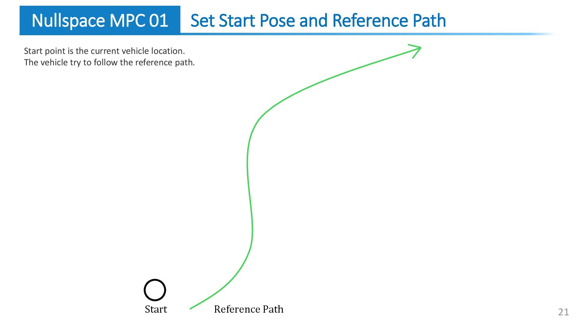
22. 22 Start Local Goal Reference Path L [m] Set Local Goal Pose Nullspace MPC 02 Set a local goal 𝐿 [m] ahead along the reference path, assuming perfect tracking.
23. Sample via poses according to gaussian distributions. There are K samples in total on each axis. 23 Start Reference Path Sample Via Poses Nullspace MPC 03 Local Goal
24. Select kth via point sample on each axis and plan a smooth trajectory trying to pass start and via points. 24 Start Reference Path Get Sample Trajectories Nullspace MPC 04 Local Goal
25. Select kth via point sample on each axis and plan a smooth trajectory trying to pass start and via points. 25 Start Reference Path Get Sample Trajectories Nullspace MPC 04 Local Goal
26. Select kth via point sample on each axis and plan a smooth trajectory trying to pass start and via points. 26 Start Reference Path Get Sample Trajectories Nullspace MPC 04 Local Goal
27. Select kth via point sample on each axis and plan a smooth trajectory trying to pass start and via points. 27 Start Reference Path Get Sample Trajectories Nullspace MPC 04 Local Goal
28. Select kth via point sample on each axis and plan a smooth trajectory trying to pass start and via points. 28 Start Reference Path Get Sample Trajectories Nullspace MPC 04 Local Goal
29. Select kth via point sample on each axis and plan a smooth trajectory trying to pass start and via points. 29 Start Reference Path Get Sample Trajectories Nullspace MPC 04 Local Goal
30. Select kth via point sample on each axis and plan a smooth trajectory trying to pass start and via points. 30 Start Reference Path Get Sample Trajectories Nullspace MPC 04 Local Goal
31. Plan smooth paths for all samples with gradient-based optimizer, and calculate cost of sample trajectories for sampling-based optimization. 31 Start Reference Path Calculate Cost for Each Sample Trajectory Nullspace MPC 05 Local Goal cost 1 = 3.07 cost 3 = 8.13 cost 2 = 2.35 cost K − 2 = 5.19 cost K = 15.3 cost K − 1 = 6.77 sample costs smaller the better Cost = costcollision_penalty +costsmooth_driving +costtracking_error +costcmd_change avoid obstacles drive smoothly track reference path accurately penalty for big command change
32. Convert sample costs into normalized weights. 32 Start Reference Path Calculate Sample Weights Nullspace MPC 06 Local Goal cost 1 = 3.07 cost 3 = 8.13 cost 2 = 2.35 cost K − 2 = 5.19 cost K = 15.3 cost K − 1 = 6.77 sample costs w 1 = 0.05 w 3 = 0.01 w 2 = 0.08 w K − 2 = 0.02 w K − 1 = 0.03 sample weights better samples get more weights w K = 0.005 Cost = costcollision_penalty +costsmooth_driving +costtracking_error +costcmd_change avoid obstacles drive smoothly track reference path accurately penalty for big command change
33. Get the Optimal Via Poses Nullspace MPC 07 Get the optimal via poses calculating the weighted sum of all sampled via poses. Start Reference Path Local Goal Prior Distribution Posterior Distribution Variational Inference 33
34. Get the Optimal Via Poses Nullspace MPC 07 Get the optimal via poses calculating the weighted sum of all sampled via poses. Start Reference Path Local Goal Prior Distribution Posterior Distribution Variational Inference 34
35. Optimal Via Poses Get the Optimal Via Poses Nullspace MPC 07 Get the optimal via poses calculating the weighted sum of all sampled via poses. Start Reference Path Local Goal 35
36. Optimal Trajectory Get the Optimal Trajectory Nullspace MPC 08 The optimal trajectory is one which passes start and optimal via points. Start Reference Path Local Goal 36
37. Simulation of Narrow Space Navigation 37 Sampling-Based MPC (MPPI) Nullspace MPC (Proposed) Nullspace MPC achieved 11% shorter trajectory length, 36% shorter travel time, with a higher success rate. Nullspace MPC required 12 times more computation time (though real-time operation was still feasible). In sequential goal-reaching simulations over 100 episodes,
38. Summary 38 How can the best motion be found across multiple tasks? Future Work • Improve computational efficiency. • Broaden applicability to more complex and realistic robotic systems, especially robots with nonlinear dynamics and high-dimensional states. Contribution • Proposed Nullspace MPC, a control framework that incorporates explicit task prioritization and accommodates diverse objectives • Demonstrated its effectiveness in narrow-space navigation of a 4WIDS vehicle, whose dynamics was approximated as holonomic motion, outperforming the MPPI controller. Strength of gradient-based approach Strength of sampling-based approach