oku-slide-20221212

Estimation of the Critical Transition Probability Using Quadratic Polynomial Approximation with Skewness Filtering
Makito Oku (University of Toyama)
2022/12/12
NOLTA 2022

Transcript

1. Estimation of the Critical Transition Probability Using Quadratic Polynomial Approximation with Skewness Filtering Makito Oku (University of Toyama) 2022/12/12 NOLTA 2022 1 / 24
2. Outline Introduction Theoretical background Estimation method Simulation settings Results Discussion and conclusions 2 / 24
3. Outline Introduction Theoretical background Estimation method Simulation settings Results Discussion and conclusions 3 / 24
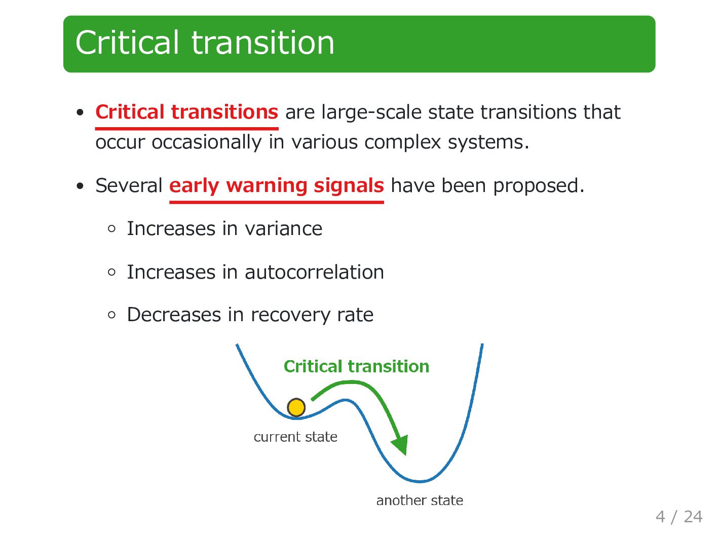
4. Critical transition Critical transitions are large-scale state transitions that occur occasionally in various complex systems. Several early warning signals have been proposed. Increases in variance Increases in autocorrelation Decreases in recovery rate 4 / 24
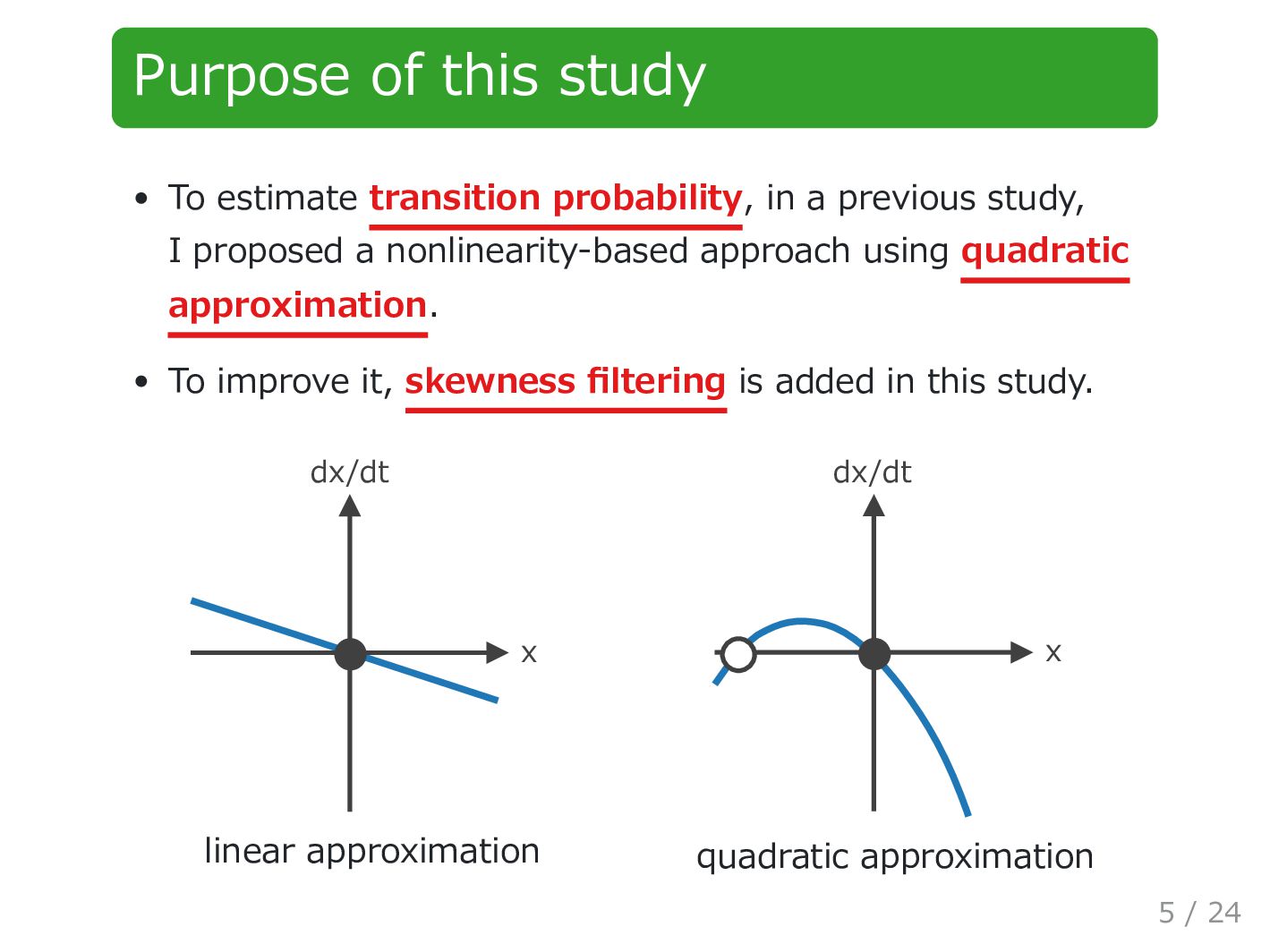
5. Purpose of this study To estimate transition probability, in a previous study, I proposed a nonlinearity-based approach using quadratic approximation. To improve it, skewness filtering is added in this study. x dx/dt linear approximation x dx/dt quadratic approximation 5 / 24
6. Outline Introduction Theoretical background Estimation method Simulation settings Results Discussion and conclusions 6 / 24
7. Assumptions Stochastic differential equation: Stable and unstable equilibrium points: and Potential function that satisfies exists. dx = f(x)dt + σ dW . xs xu U f = −U ′ 7 / 24
8. Mean escape time Approximated mean escape time (C. Gardiner, 1985) Transition probability: T = 2π √−f ′ (xs )f ′ (xu ) exp ( 2 σ2 (U (x u ) − U (x s ))). P (y ≤ t) = 1 − exp(−t/T ). 8 / 24
9. Quasi-stationary distribution Quasi-stationary distribution before transition can be approximated by the Boltzmann distribution: p(x) = 1 Z exp (− 2 σ2 U (x)), x > x u . 9 / 24
10. Outline Introduction Theoretical background Estimation method Simulation settings Results Discussion and conclusions 10 / 24
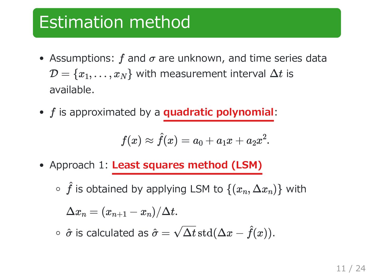
11. Estimation method Assumptions: and are unknown, and time series data with measurement interval is available. is approximated by a quadratic polynomial: Approach 1: Least squares method (LSM) is obtained by applying LSM to with is calculated as . f σ D = {x1 , … , xN } Δt f f(x) ≈ ^ f(x) = a0 + a1 x + a2 x 2 . ^ f {(xn , Δxn )} Δxn = (xn+1 − xn )/Δt. ^ σ ^ σ = √Δt std(Δx − ^ f(x)) 11 / 24
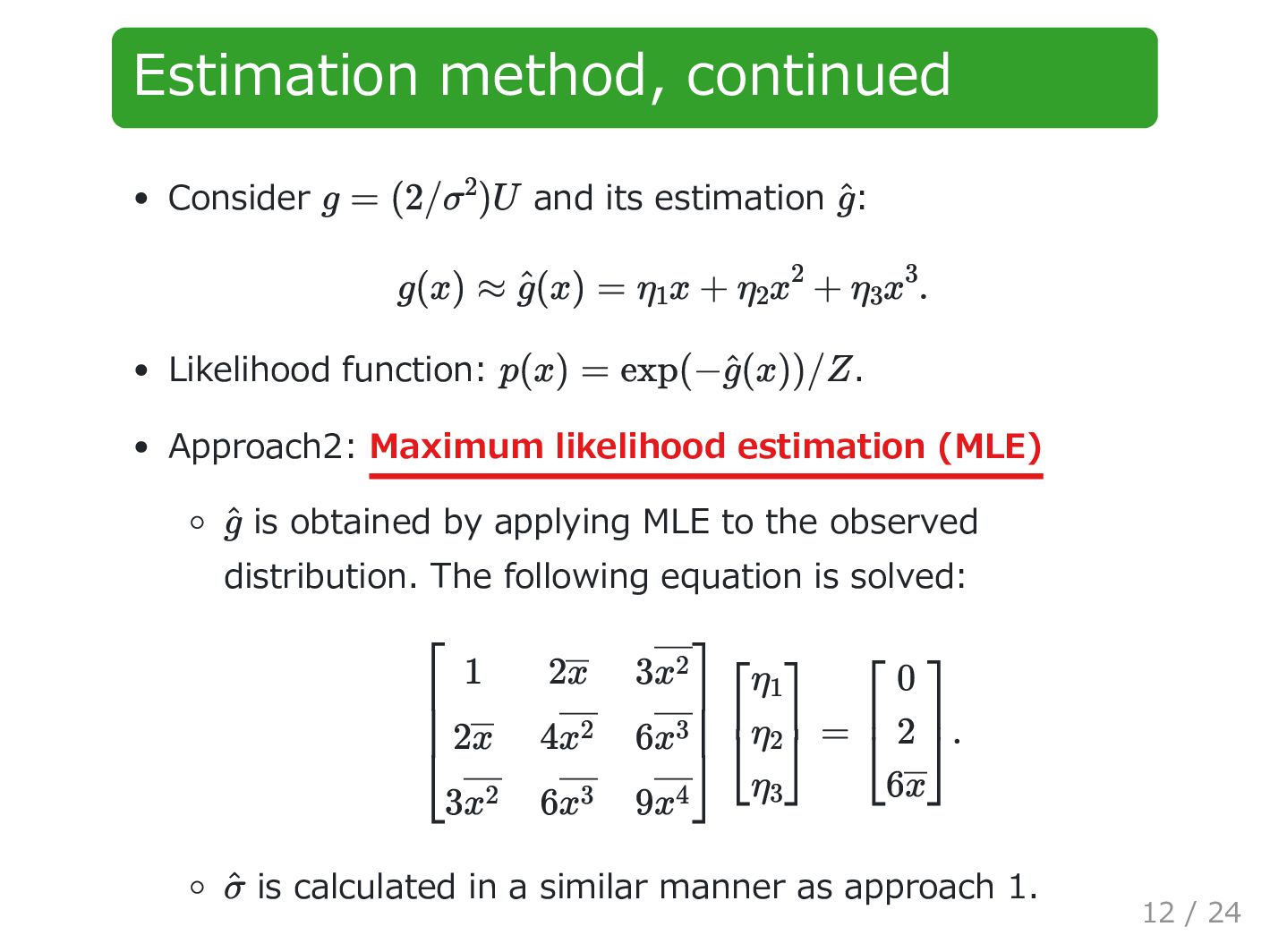
12. Estimation method, continued Consider and its estimation : Likelihood function: . Approach2: Maximum likelihood estimation (MLE) is obtained by applying MLE to the observed distribution. The following equation is solved: is calculated in a similar manner as approach 1. g = (2/σ 2 )U ^ g g(x) ≈ ^ g(x) = η1 x + η2 x 2 + η3 x 3 . p(x) = exp(−^ g(x))/Z ^ g = . ⎡ ⎣ 1 2x 3x2 2x 4x2 6x3 3x2 6x3 9x4 ⎤ ⎦ ⎡ ⎣ η1 η2 η3 ⎤ ⎦ ⎡ ⎣ 0 2 6x ⎤ ⎦ ^ σ 12 / 24
13. Skewness filtering Skewness filtering is introduced as a reject option. When skewness is below , prediction is made. Otherwise, prediction is not made. θ 13 / 24
14. Outline Introduction Theoretical background Estimation method Simulation settings Results Discussion and conclusions 14 / 24
15. May model May model (R. May, 1977) We can set without loss of generality. dx dt = f(x) = r x (1 − x K ) − c x 2 x2 + h2 . r = K = 1 15 / 24
16. Simulation settings May model's parameters: and Bifurcation point is . Euler-Maruyama method , , and . Resampling with interval h = 0.1 c = 0.257 c ≃ 0.260 Δxn+1 = f(xn )Δt + σ√Δt ξn . Δt = 0.1 σ = 0.01 x0 = x s ≃ 0.539 k x1 , x2 , x3 , … ⇒ x1 , x1+k , x1+2k , … 16 / 24
17. Outline Introduction Theoretical background Estimation method Simulation settings Results Discussion and conclusions 17 / 24
18. Distribution of skewness We can read the probability of making a prediction for given and . For example, more than 20 % cases meet the criterion when and . θ N θ = −0.5 N = 10 5 18 / 24
19. Threshold and prediction error The absolute error tended to increase as increased. The precision was similar between LSM and MLE for and . was about % for and . θ θ N = 10 4 N = 10 5 ^ T /T ±50 θ = −0.5 N = 10 5 19 / 24
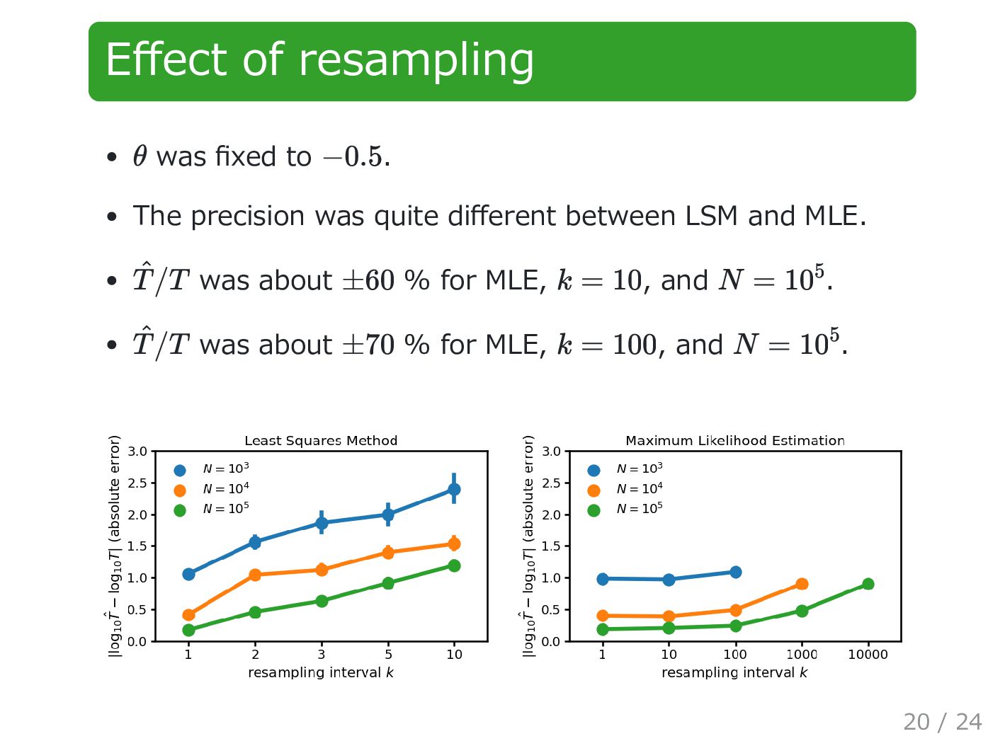
20. Effect of resampling was fixed to . The precision was quite different between LSM and MLE. was about % for MLE, , and . was about % for MLE, , and . θ −0.5 ^ T /T ±60 k = 10 N = 10 5 ^ T /T ±70 k = 100 N = 10 5 20 / 24
21. Outline Introduction Theoretical background Estimation method Simulation settings Results Discussion and conclusions 21 / 24
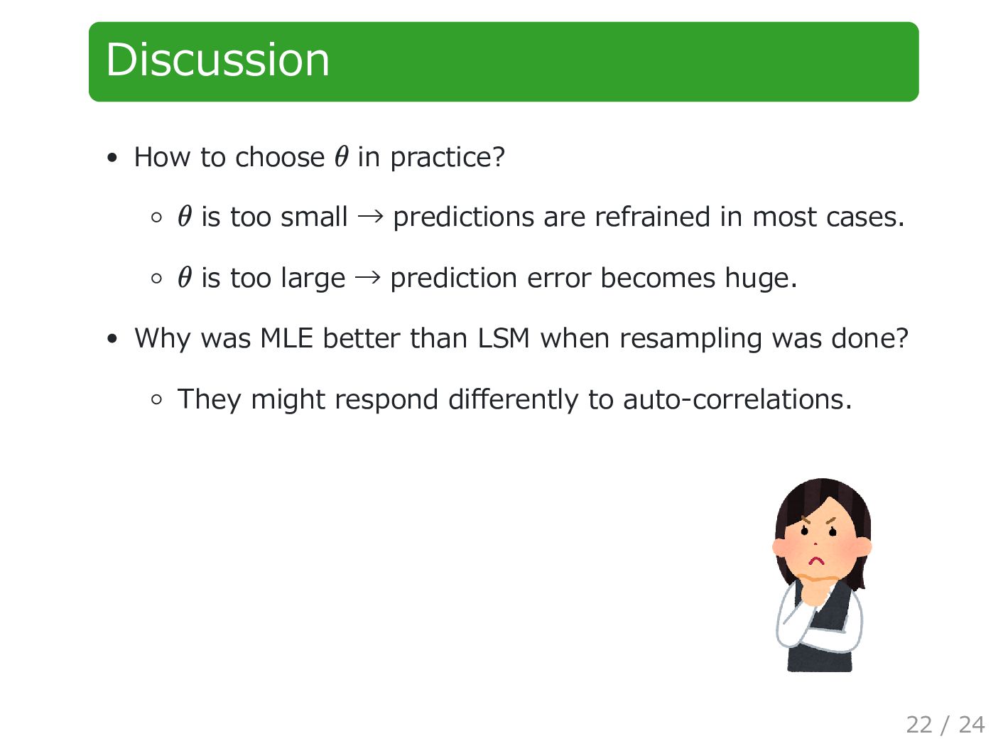
22. Discussion How to choose in practice? is too small → predictions are refrained in most cases. is too large → prediction error becomes huge. Why was MLE better than LSM when resampling was done? They might respond differently to auto-correlations. θ θ θ 22 / 24
23. Conclusions I have proposed a method for estimating critical transition probability using quadratic polynomial approximation with skewness filtering. The proposed method was applied to May model. The results of numerical simulations showed that the proposed method worked well. It was also found that MLE required much less data points than LSM if auto-correlation was weak ( ). k > 1 23 / 24
24. Thank you for your attention! 24 / 24