Operations on Genomic Intervals and Genome Arithmetic

【第6回】ゼロから始めるゲノム解析（R編）

Transcript

1. Operations on Genomic Intervals and Genome Arithmetic 第6回ゼロから始めるゲノム解析（後半） onouyek@2020年12月4日
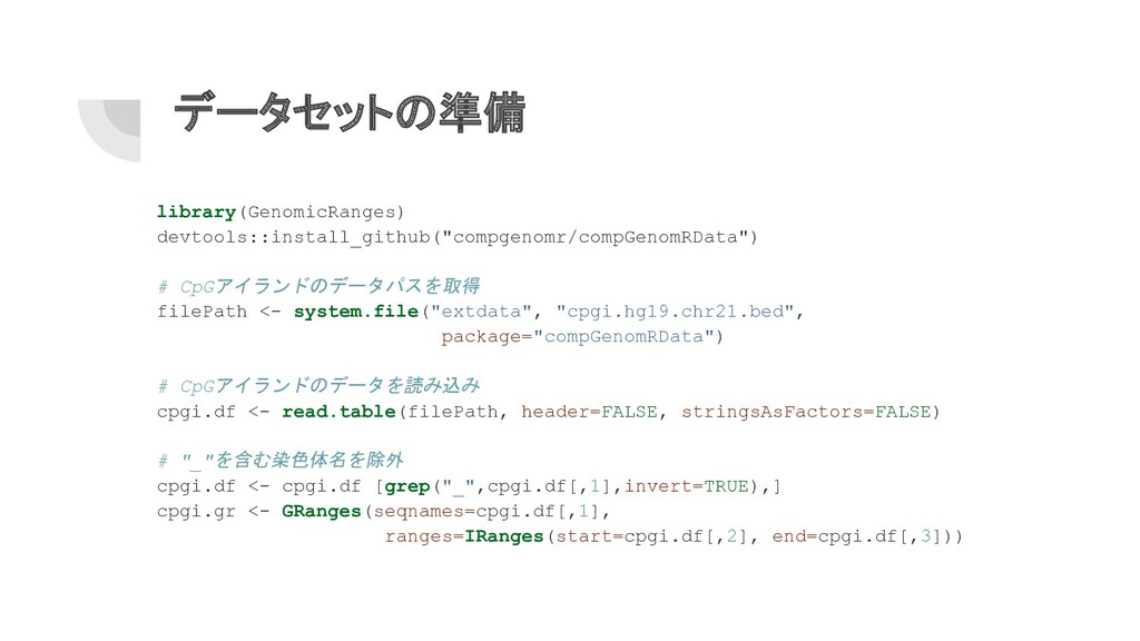
2. データセットの準備 library(GenomicRanges) devtools::install_github("compgenomr/compGenomRData") # CpGアイランドのデータパスを取得 filePath <- system.file("extdata", "cpgi.hg19.chr21.bed", package="compGenomRData") # CpGアイランドのデータを読み込み cpgi.df <- read.table(filePath, header=FALSE, stringsAsFactors=FALSE) # "_"を含む染色体名を除外 cpgi.df <- cpgi.df [grep("_",cpgi.df[,1],invert=TRUE),] cpgi.gr <- GRanges(seqnames=cpgi.df[,1], ranges=IRanges(start=cpgi.df[,2], end=cpgi.df[,3]))
3. 詳細情報を含む ゲノム間隔 Genomic intervals with more information
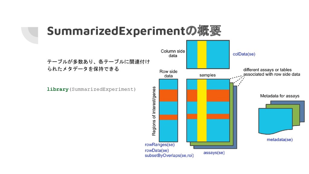
4. SummarizedExperimentの概要 テーブルが多数あり、各テーブルに関連付け られたメタデータを保持できる library(SummarizedExperiment)
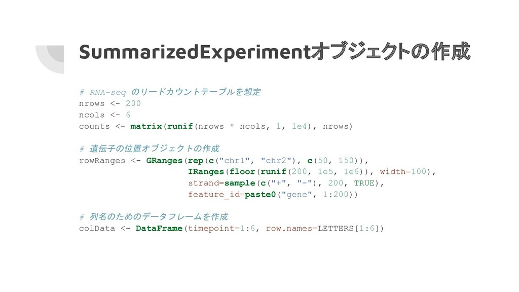
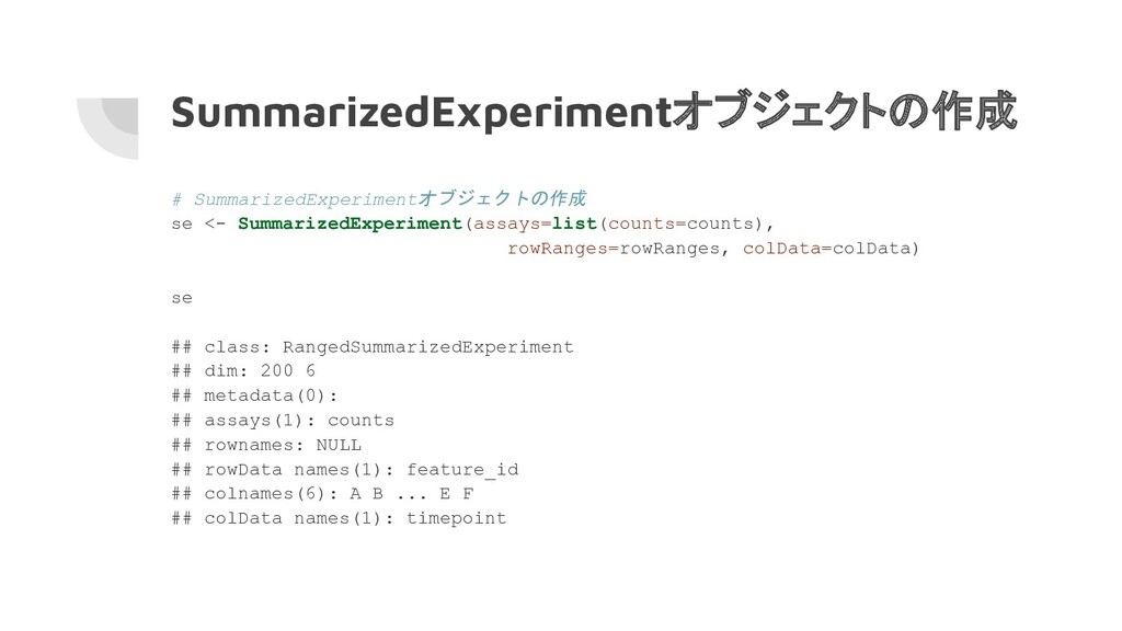
5. SummarizedExperimentオブジェクトの作成 # RNA-seq のリードカウントテーブルを想定 nrows <- 200 ncols <- 6 counts <- matrix(runif(nrows * ncols, 1, 1e4), nrows) # 遺伝子の位置オブジェクトの作成 rowRanges <- GRanges(rep(c("chr1", "chr2"), c(50, 150)), IRanges(floor(runif(200, 1e5, 1e6)), width=100), strand=sample(c("+", "-"), 200, TRUE), feature_id=paste0("gene", 1:200)) # 列名のためのデータフレームを作成 colData <- DataFrame(timepoint=1:6, row.names=LETTERS[1:6])
6. SummarizedExperimentオブジェクトの作成 # SummarizedExperimentオブジェクトの作成 se <- SummarizedExperiment(assays=list(counts=counts), rowRanges=rowRanges, colData=colData) se ## class: RangedSummarizedExperiment ## dim: 200 6 ## metadata(0): ## assays(1): counts ## rownames: NULL ## rowData names(1): feature_id ## colnames(6): A B ... E F ## colData names(1): timepoint
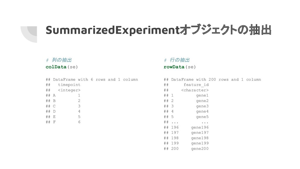
7. SummarizedExperimentオブジェクトの抽出 # 列の抽出 colData(se) ## DataFrame with 6 rows and 1 column ## timepoint ## <integer> ## A 1 ## B 2 ## C 3 ## D 4 ## E 5 ## F 6 # 行の抽出 rowData(se) ## DataFrame with 200 rows and 1 column ## feature_id ## <character> ## 1 gene1 ## 2 gene2 ## 3 gene3 ## 4 gene4 ## 5 gene5 ## ... ... ## 196 gene196 ## 197 gene197 ## 198 gene198 ## 199 gene199 ## 200 gene200
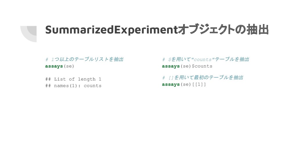
8. SummarizedExperimentオブジェクトの抽出 # 1つ以上のテーブルリストを抽出 assays(se) ## List of length 1 ## names(1): counts # $を用いて"counts"テーブルを抽出 assays(se)$counts # []を用いて最初のテーブルを抽出 assays(se)[[1]]
9. SummarizedExperimentオブジェクトのサブ セット化 # 最初の5つの転写物と最初の3つのサンプルを サブセット化 se[1:5, 1:3] ## class: RangedSummarizedExperiment ## dim: 5 3 ## metadata(0): ## assays(1): counts ## rownames: NULL ## rowData names(1): feature_id ## colnames(3): A B C ## colData names(1): timepoint # chr1:100,000-1,100,000の行でサブセット化 roi <- GRanges(seqnames="chr1", ranges=100000:1100000) subsetByOverlaps(se, roi) ## class: RangedSummarizedExperiment ## dim: 50 6 ## metadata(0): ## assays(1): counts ## rownames: NULL ## rowData names(1): feature_id ## colnames(6): A B ... E F ## colData names(1): timepoint
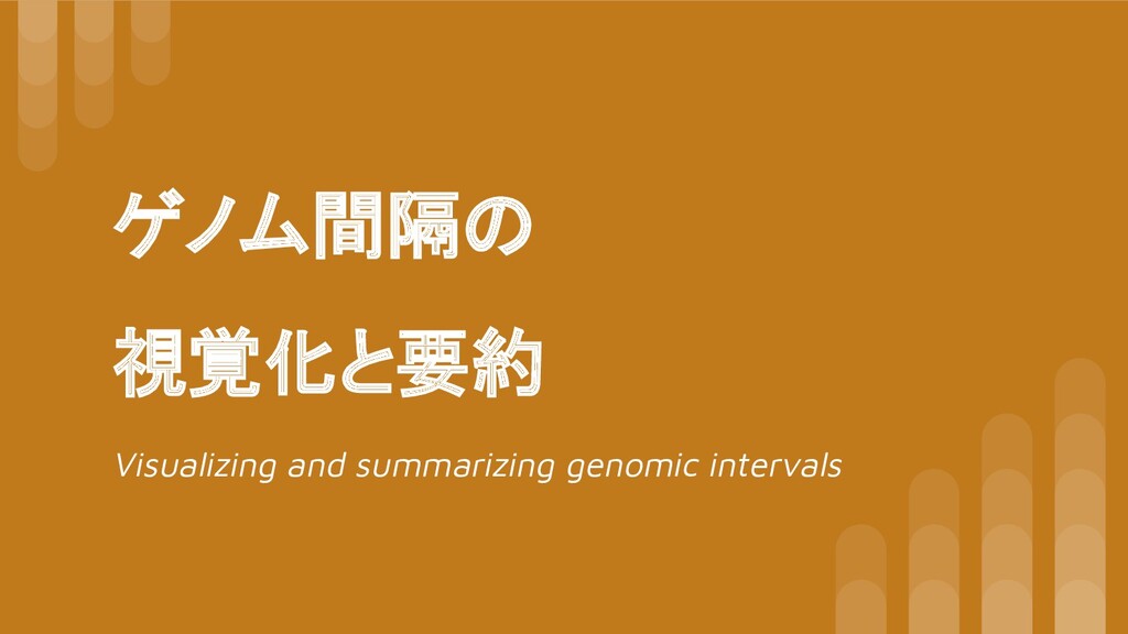
10. ゲノム間隔の 視覚化と要約 Visualizing and summarizing genomic intervals
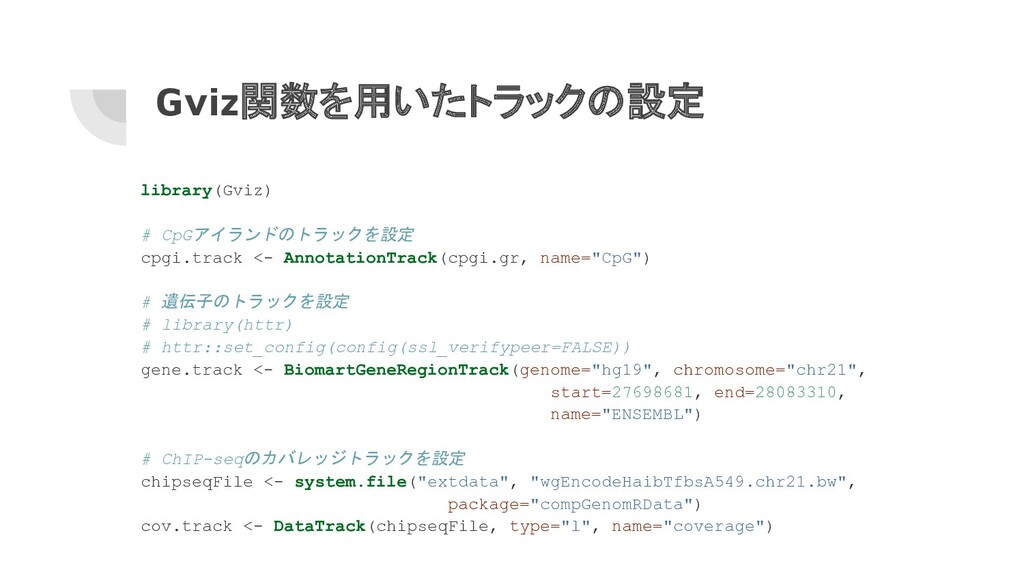
11. Gviz関数を用いたトラックの設定 library(Gviz) # CpGアイランドのトラックを設定 cpgi.track <- AnnotationTrack(cpgi.gr, name="CpG") # 遺伝子のトラックを設定 # library(httr) # httr::set_config(config(ssl_verifypeer=FALSE)) gene.track <- BiomartGeneRegionTrack(genome="hg19", chromosome="chr21", start=27698681, end=28083310, name="ENSEMBL") # ChIP-seqのカバレッジトラックを設定 chipseqFile <- system.file("extdata", "wgEncodeHaibTfbsA549.chr21.bw", package="compGenomRData") cov.track <- DataTrack(chipseqFile, type="l", name="coverage")
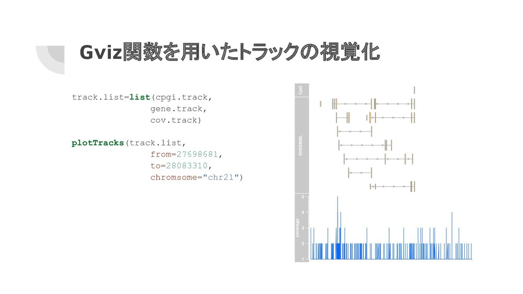
12. Gviz関数を用いたトラックの視覚化 track.list=list(cpgi.track, gene.track, cov.track) plotTracks(track.list, from=27698681, to=28083310, chromsome="chr21")
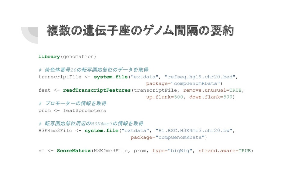
13. 複数の遺伝子座のゲノム間隔の要約 library(genomation) # 染色体番号20の転写開始部位のデータを取得 transcriptFile <- system.file("extdata", "refseq.hg19.chr20.bed", package="compGenomRData") feat <- readTranscriptFeatures(transcriptFile, remove.unusual=TRUE, up.flank=500, down.flank=500) # プロモーターの情報を取得 prom <- feat$promoters # 転写開始部位周辺のH3K4me3の情報を取得 H3K4me3File <- system.file("extdata", "H1.ESC.H3K4me3.chr20.bw", package="compGenomRData") sm <- ScoreMatrix(H3K4me3File, prom, type="bigWig", strand.aware=TRUE)
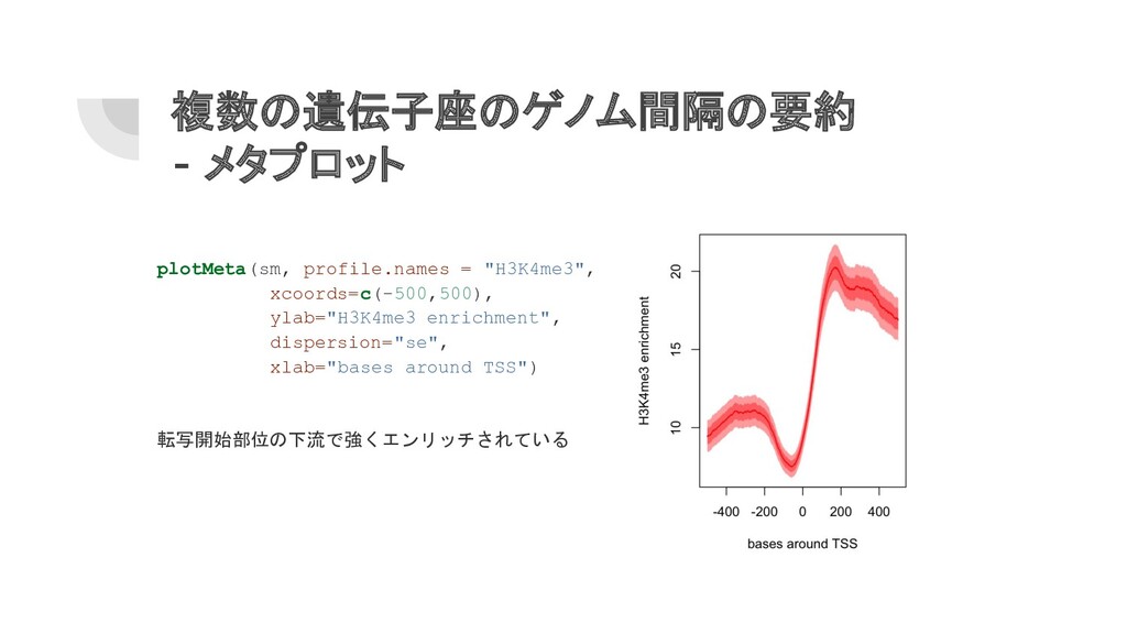
14. 複数の遺伝子座のゲノム間隔の要約 - メタプロット plotMeta(sm, profile.names = "H3K4me3", xcoords=c(-500,500), ylab="H3K4me3 enrichment", dispersion="se", xlab="bases around TSS") 転写開始部位の下流で強くエンリッチされている
15. 複数の遺伝子座のゲノム間隔の要約 - ヒートマップ heatMatrix(sm, order=TRUE, xcoords=c(-500,500), xlab="bases around TSS") 各行が転写開始部位周囲の領域 エンリッチメントの強度で色分けされている
16. 複数の遺伝子座のゲノム間隔の要約 - メタプロットの組み合わせ # DNAseのデータを組み合わせる DNAseFile <- system.file("extdata", "H1.ESC.dnase.chr20.bw", package="compGenomRData") sml <- ScoreMatrixList(c(H3K4me3=H3K4me3File, DNAse=DNAseFile), prom, type="bigWig", strand.aware=TRUE) plotMeta(sml)
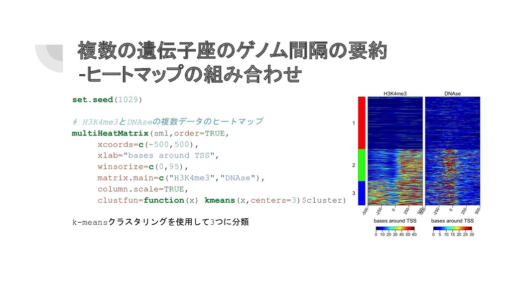
17. 複数の遺伝子座のゲノム間隔の要約 -ヒートマップの組み合わせ set.seed(1029) # H3K4me3とDNAseの複数データのヒートマップ multiHeatMatrix(sml,order=TRUE, xcoords=c(-500,500), xlab="bases around TSS", winsorize=c(0,95), matrix.main=c("H3K4me3","DNAse"), column.scale=TRUE, clustfun=function(x) kmeans(x,centers=3)$cluster) k-meansクラスタリングを使用して3つに分類
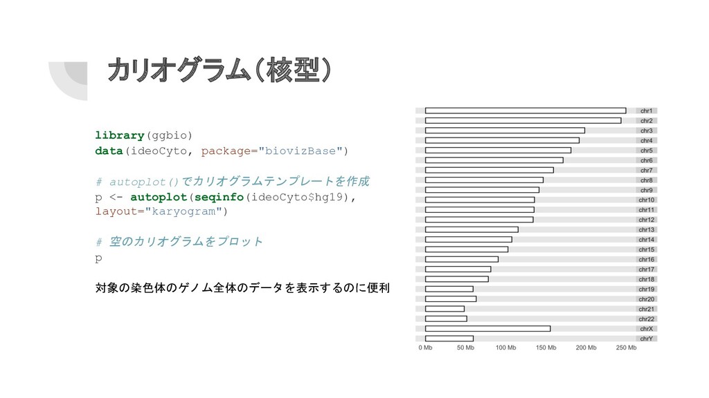
18. カリオグラム（核型） library(ggbio) data(ideoCyto, package="biovizBase") # autoplot()でカリオグラムテンプレートを作成 p <- autoplot(seqinfo(ideoCyto$hg19), layout="karyogram") # 空のカリオグラムをプロット p 対象の染色体のゲノム全体のデータを表示するのに便利
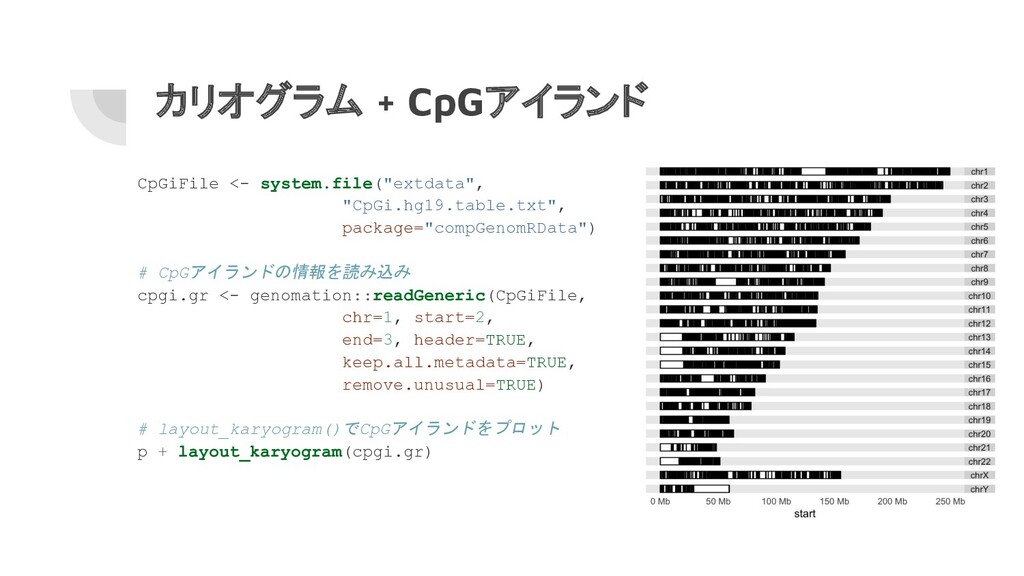
19. カリオグラム + CpGアイランド CpGiFile <- system.file("extdata", "CpGi.hg19.table.txt", package="compGenomRData") # CpGアイランドの情報を読み込み cpgi.gr <- genomation::readGeneric(CpGiFile, chr=1, start=2, end=3, header=TRUE, keep.all.metadata=TRUE, remove.unusual=TRUE) # layout_karyogram()でCpGアイランドをプロット p + layout_karyogram(cpgi.gr)
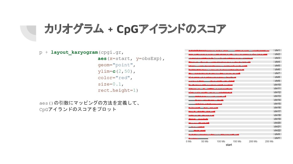
20. カリオグラム + CpGアイランドのスコア p + layout_karyogram(cpgi.gr, aes(x=start, y=obsExp), geom="point", ylim=c(2,50), color="red", size=0.1, rect.height=1) aes()の引数にマッピングの方法を定義して、 CpGアイランドのスコアをプロット
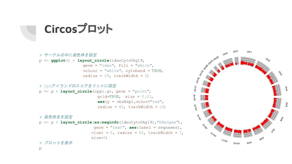
21. Circosプロット # サークルの中に染色体を設定 p <- ggplot() + layout_circle(ideoCyto$hg19, geom = "ideo", fill = "white", colour = "white", cytoband = TRUE, radius = 39, trackWidth = 2) # CpGアイランドのスコアをドットに設定 p <- p + layout_circle(cpgi.gr, geom = "point", grid=TRUE,　size = 0.01, aes(y = obsExp),color="red", radius = 42, trackWidth = 10) # 染色体名を設定 p <- p + layout_circle(as(seqinfo(ideoCyto$hg19),"GRanges"), geom = "text", aes(label = seqnames), vjust = 0, radius = 55, trackWidth = 7, size=3) # プロットを表示 p