Reduction in Parameter Studies This material is based upon work supported by the U.S. Department of Energy Office of Science, Office of Advanced Scientific Computing Research, Applied Mathematics program under Award Number DE-SC-0011077. Thanks to: David Gleich Purdue, CS PAUL CONSTANTINE Ben L. Fryrear Assistant Professor Applied Mathematics & Statistics Colorado School of Mines activesubspaces.org! @DrPaulynomial! SLIDES: DISCLAIMER: These slides are meant to complement the oral presentation. Use out of context at your own risk.
Iaccarino, J. Larsson, M. Emory) Sensitivity analysis in hydrological models (with R. Maxwell, J. Jefferson, J. Gilbert) Shape optimization in aerospace vehicles (with J. Alonso, T. Lukaczyk)
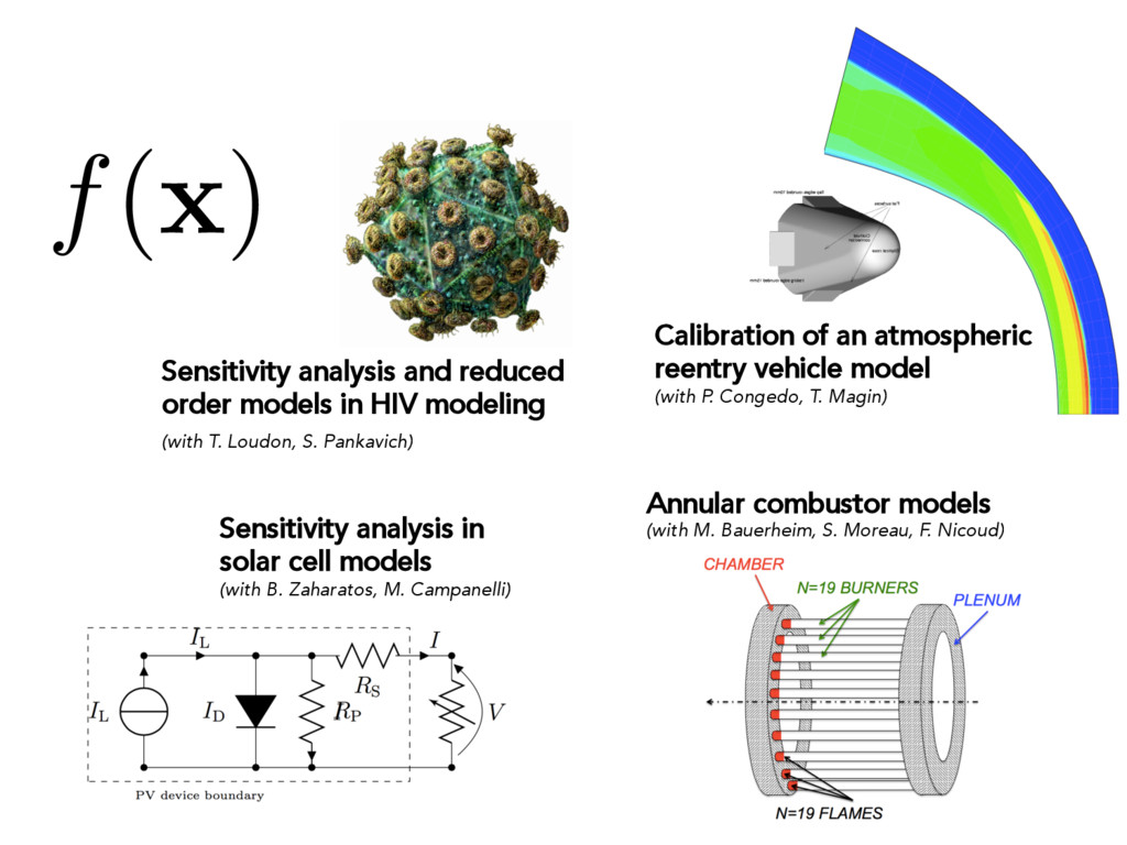
B. Zaharatos, M. Campanelli) Sensitivity analysis and reduced order models in HIV modeling (with T. Loudon, S. Pankavich) Annular combustor models (with M. Bauerheim, S. Moreau, F. Nicoud) Calibration of an atmospheric reentry vehicle model (with P. Congedo, T. Magin)
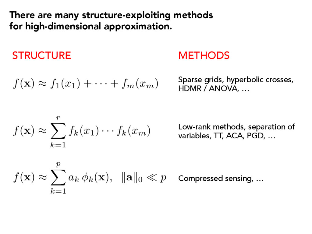
), k a k0 ⌧ p f ( x ) ⇡ f1( x1) + · · · + fm( xm) There are many structure-exploiting methods for high-dimensional approximation. STRUCTURE METHODS Sparse grids, hyperbolic crosses, HDMR / ANOVA, … f ( x ) ⇡ r X k=1 fk( x1) · · · fk( xm) Low-rank methods, separation of variables, TT, ACA, PGD, … Compressed sensing, …
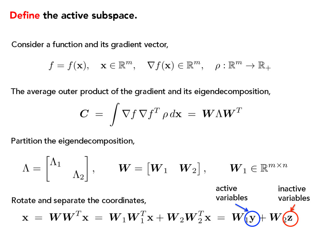
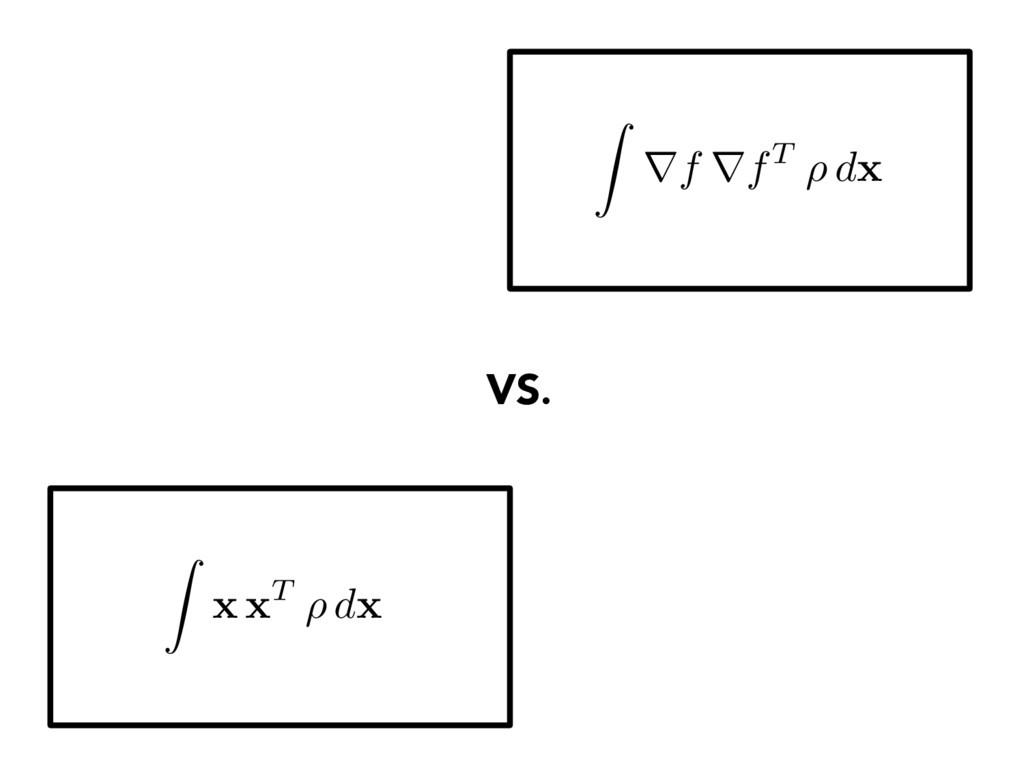
vector, The average outer product of the gradient and its eigendecomposition, Partition the eigendecomposition, Rotate and separate the coordinates, ⇤ = ⇤1 ⇤2 , W = ⇥ W 1 W 2 ⇤ , W 1 2 Rm⇥n x = W W T x = W 1W T 1 x + W 2W T 2 x = W 1y + W 2z active variables inactive variables f = f( x ), x 2 Rm, rf( x ) 2 Rm, ⇢ : Rm ! R + C = Z rf rfT ⇢ d x = W ⇤W T
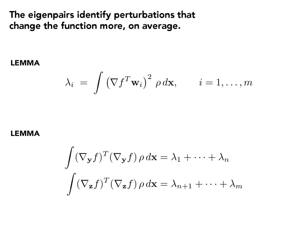
i = 1, . . . , m The eigenpairs identify perturbations that change the function more, on average. LEMMA LEMMA Z (ryf)T (ryf) ⇢ d x = 1 + · · · + n Z (rzf)T (rzf) ⇢ d x = n+1 + · · · + m
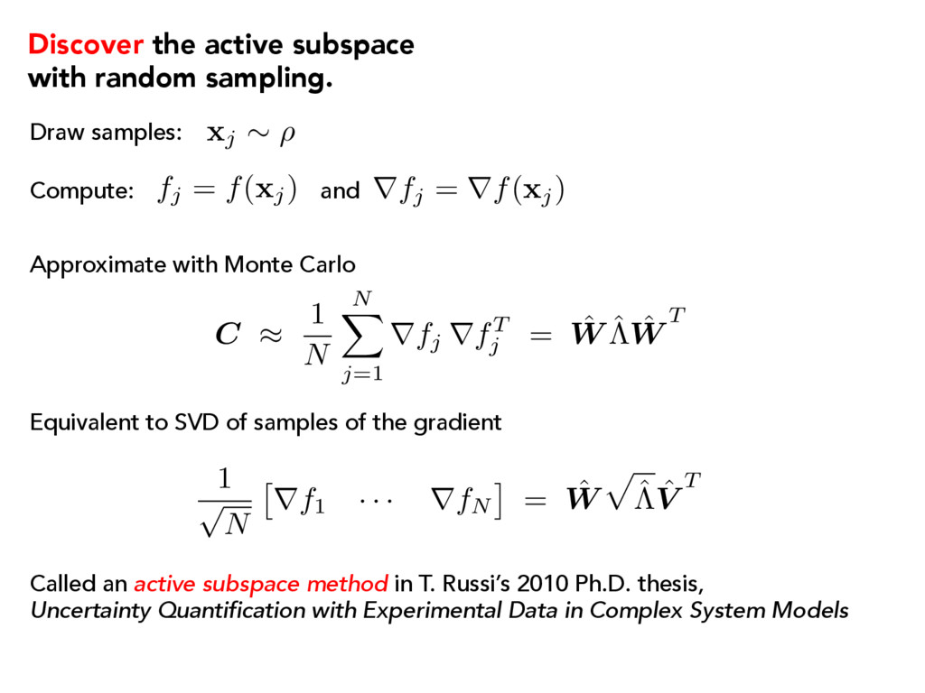
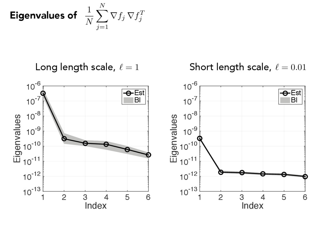
and fj = f( xj) Approximate with Monte Carlo Equivalent to SVD of samples of the gradient Called an active subspace method in T. Russi’s 2010 Ph.D. thesis, Uncertainty Quantification with Experimental Data in Complex System Models xj ⇠ ⇢ C ⇡ 1 N N X j=1 rfj rfT j = ˆ W ˆ ⇤ ˆ W T 1 p N ⇥ rf1 · · · rfN ⇤ = ˆ W p ˆ ⇤ ˆ V T rfj = rf( xj)
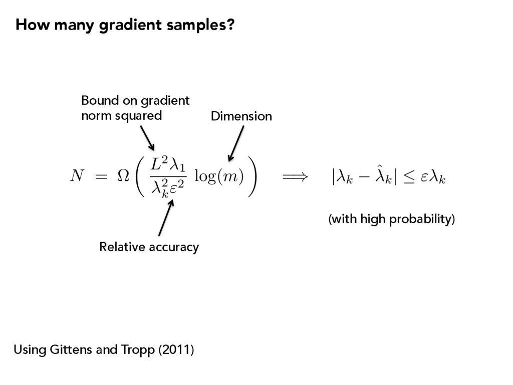
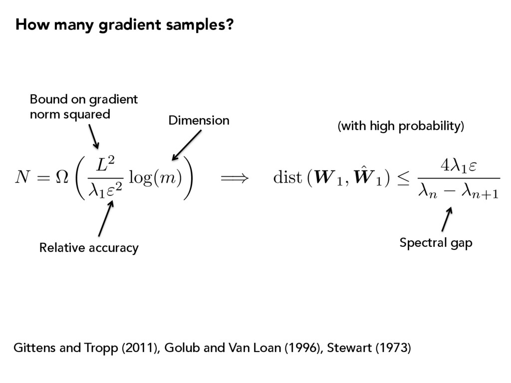
(1973) Bound on gradient norm squared Relative accuracy Dimension (with high probability) Spectral gap N = ⌦ ✓ L2 1"2 log( m ) ◆ = ) dist ( W 1, ˆ W 1) 4 1" n n+1 How many gradient samples?
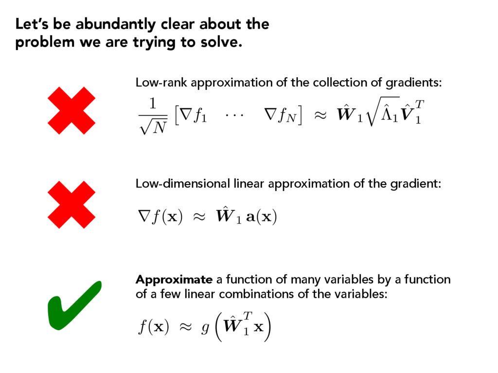
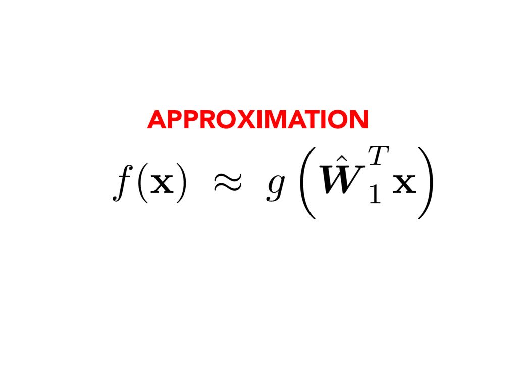
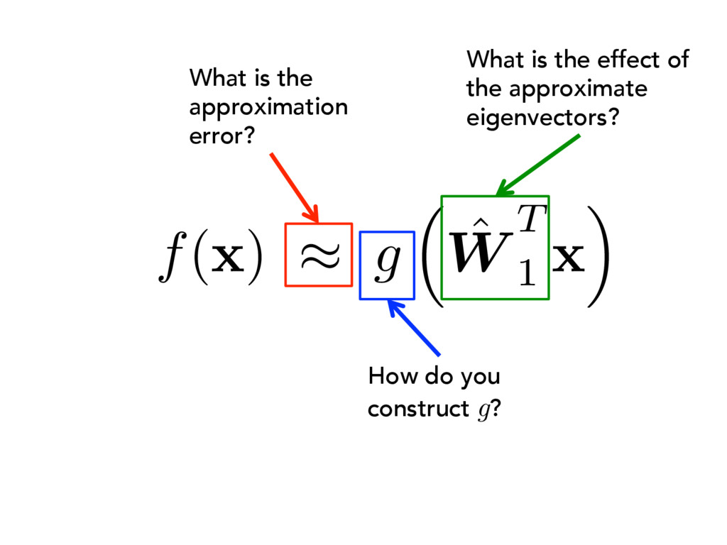
⇡ ˆ W 1 q ˆ ⇤1 ˆ V T 1 Low-rank approximation of the collection of gradients: Let’s be abundantly clear about the problem we are trying to solve. Low-dimensional linear approximation of the gradient: rf( x ) ⇡ ˆ W 1 a ( x ) f( x ) ⇡ g ⇣ ˆ W T 1 x ⌘ Approximate a function of many variables by a function of a few linear combinations of the variables: ✔ ✖ ✖
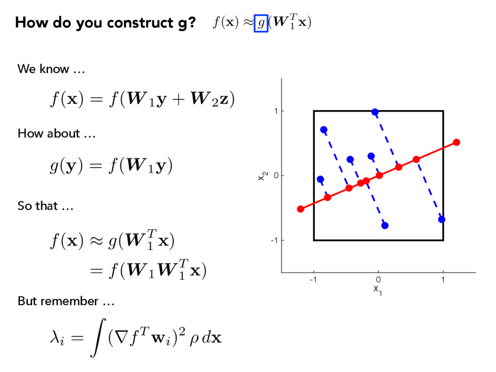
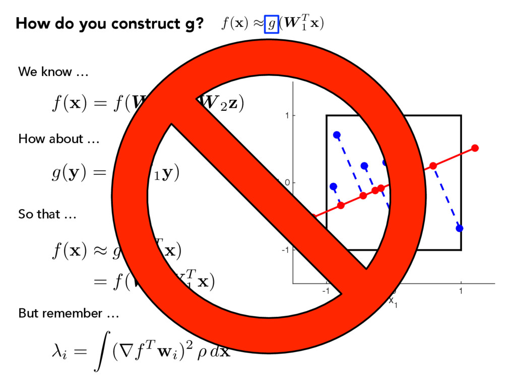
1y + W 2z ) g(y) = f(W 1y) f( x ) ⇡ g(W T 1 x ) = f(W 1W T 1 x ) f( x ) ⇡ g (W T 1 x ) We know … How about … So that … x 1 -1 0 1 x 2 -1 0 1 But remember … i = Z (rfT wi)2 ⇢ d x
1y + W 2z ) g(y) = f(W 1y) f( x ) ⇡ g(W T 1 x ) = f(W 1W T 1 x ) f( x ) ⇡ g (W T 1 x ) We know … How about … So that … x 1 -1 0 1 x 2 -1 0 1 But remember … i = Z (rfT wi)2 ⇢ d x
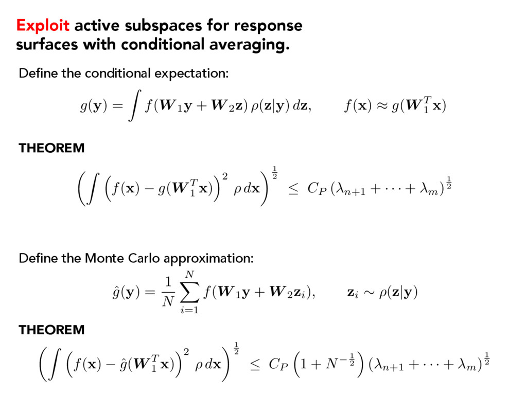
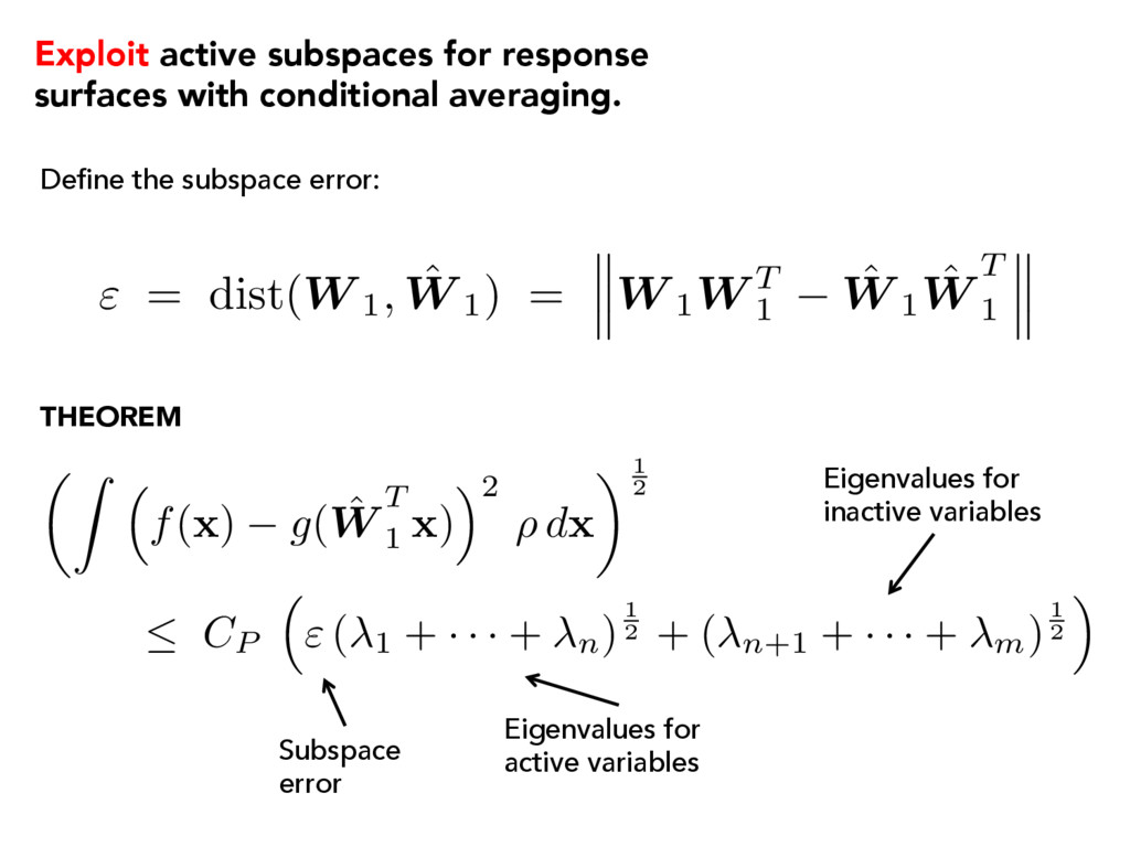
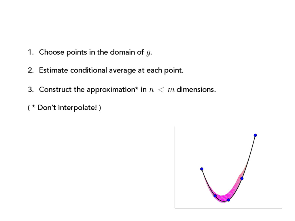
g( y ) = Z f(W 1y + W 2z ) ⇢( z | y ) d z , f( x ) ⇡ g(W T 1 x ) ˆ g(y) = 1 N N X i=1 f(W 1y + W 2zi), zi ⇠ ⇢(z|y) Exploit active subspaces for response surfaces with conditional averaging. ✓Z ⇣ f( x ) g(W T 1 x ) ⌘2 ⇢ d x ◆1 2 CP ( n+1 + · · · + m)1 2 ✓Z ⇣ f( x ) ˆ g(W T 1 x ) ⌘2 ⇢ d x ◆1 2 CP ⇣ 1 + N 1 2 ⌘ ( n+1 + · · · + m)1 2 THEOREM
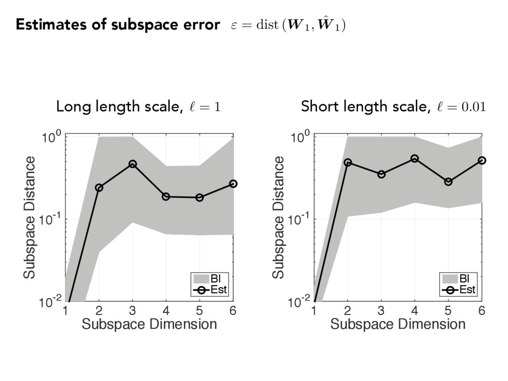
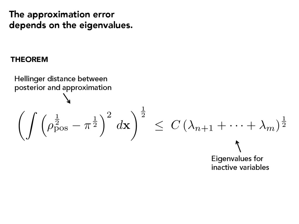
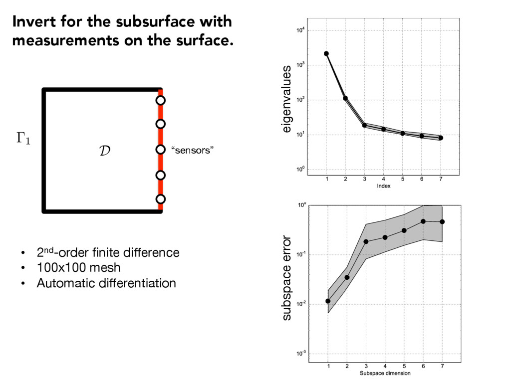
T 1 ˆ W 1 ˆ W T 1 ✓Z ⇣ f( x ) g( ˆ W T 1 x ) ⌘2 ⇢ d x ◆1 2 CP ⇣ " ( 1 + · · · + n)1 2 + ( n+1 + · · · + m)1 2 ⌘ Subspace error Eigenvalues for active variables Eigenvalues for inactive variables Define the subspace error: THEOREM Exploit active subspaces for response surfaces with conditional averaging.
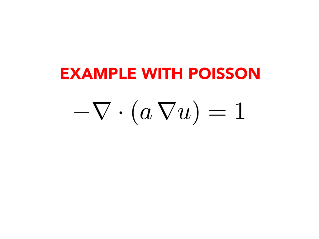
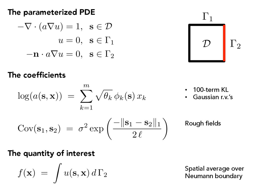
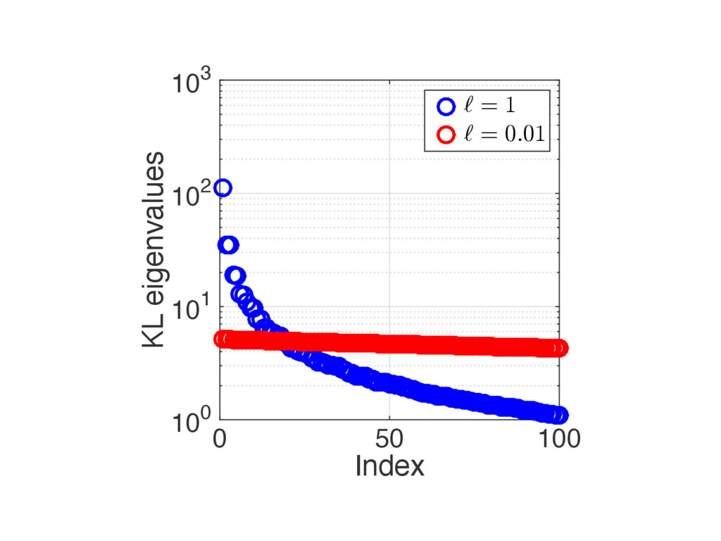
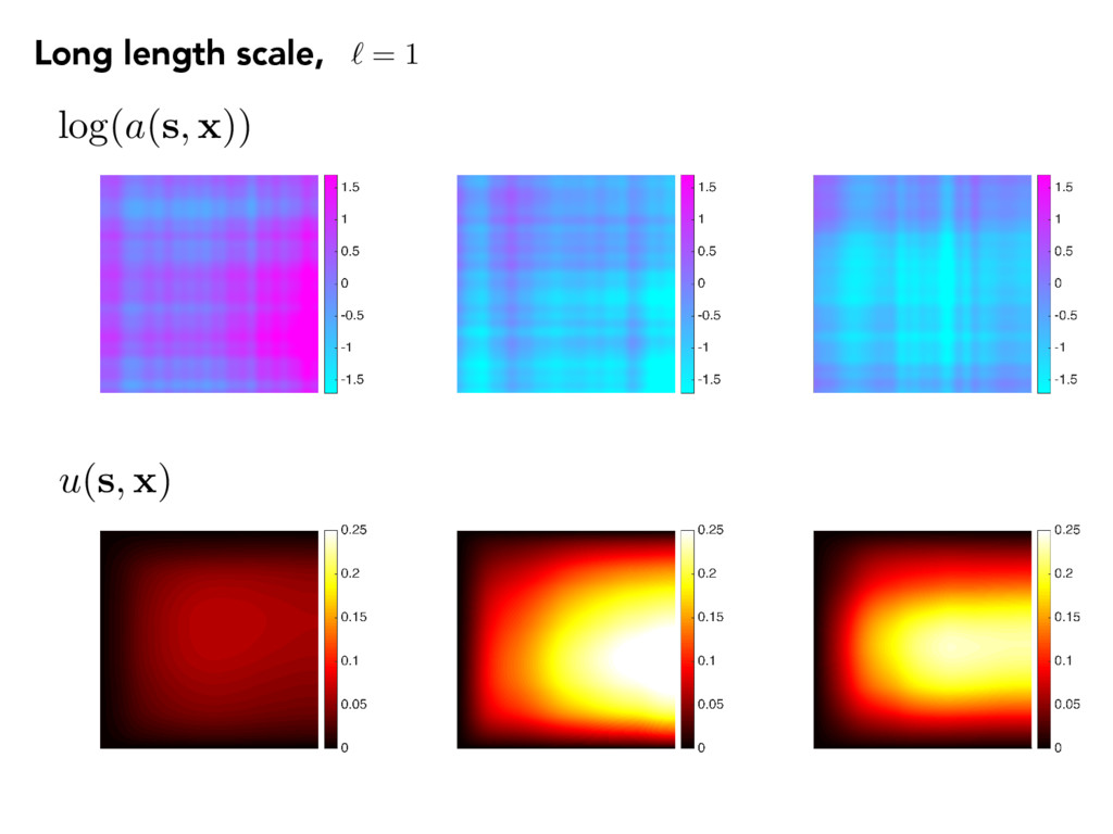
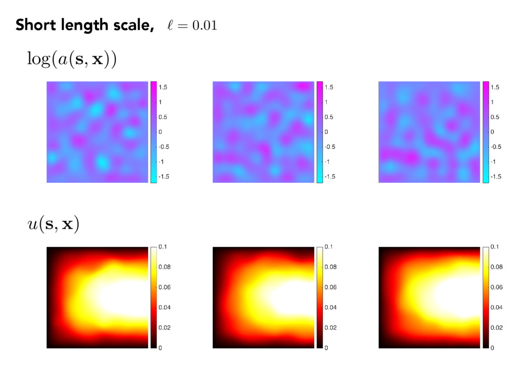
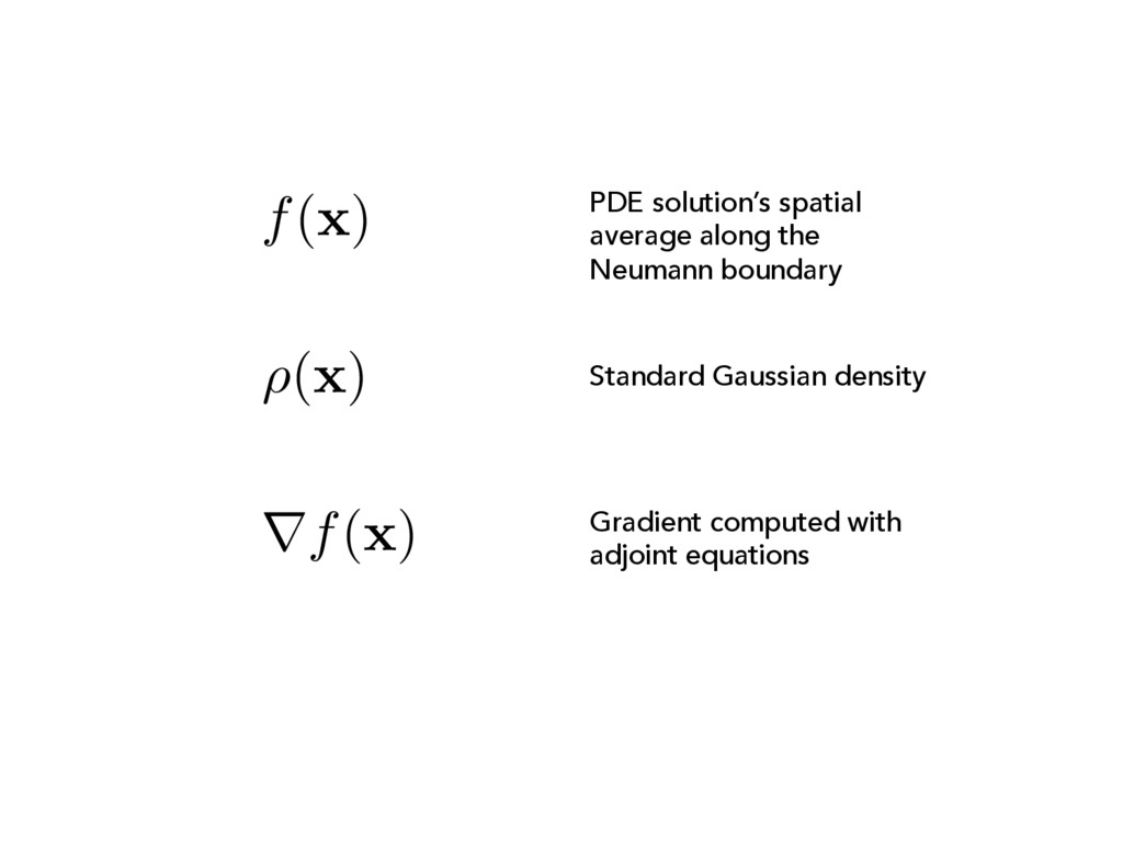
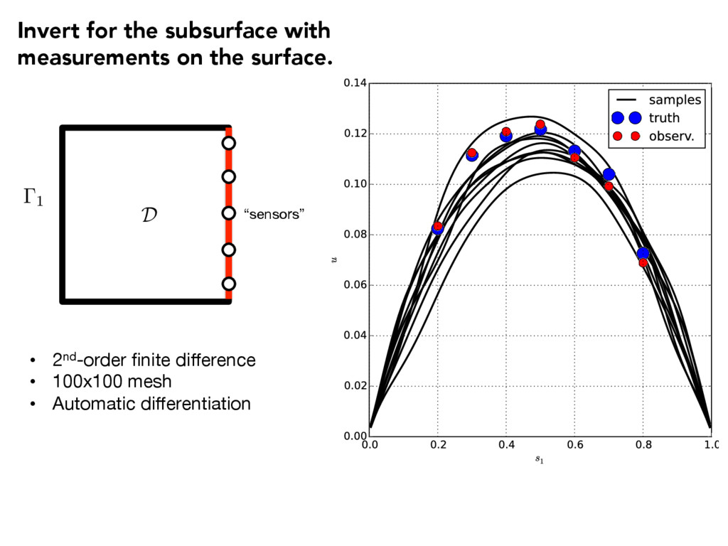
(aru) = 1, s 2 D u = 0, s 2 1 n · aru = 0, s 2 2 log(a(s, x)) = m X k=1 p ✓k k(s) xk Cov( s1, s2) = 2 exp ✓ ks1 s2 k1 2 ` ◆ The quantity of interest f( x ) = Z u( s , x ) d 2 • 100-term KL • Gaussian r.v.’s Rough fields Spatial average over Neumann boundary
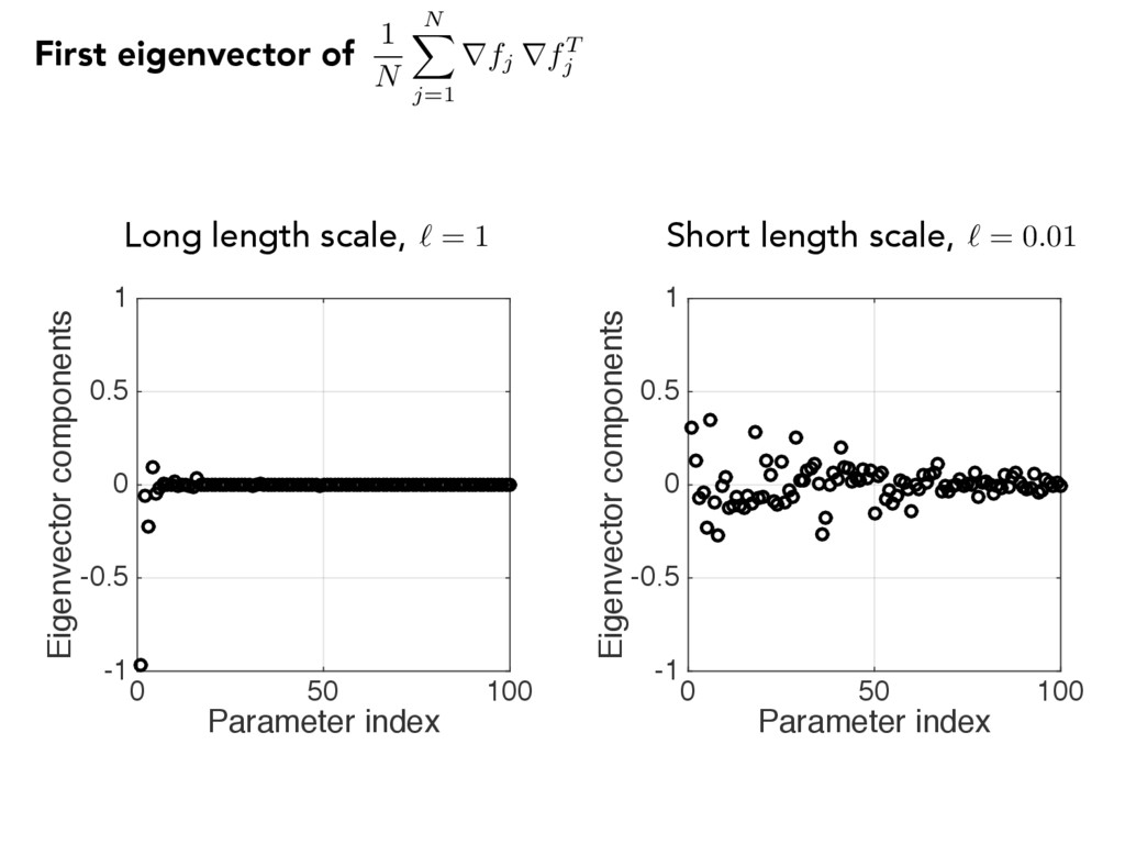
0.5 1 Parameter index 0 50 100 Eigenvector components -1 -0.5 0 0.5 1 First eigenvector of Long length scale, ` = 1 Short length scale, ` = 0.01 1 N N X j=1 rfj rfT j
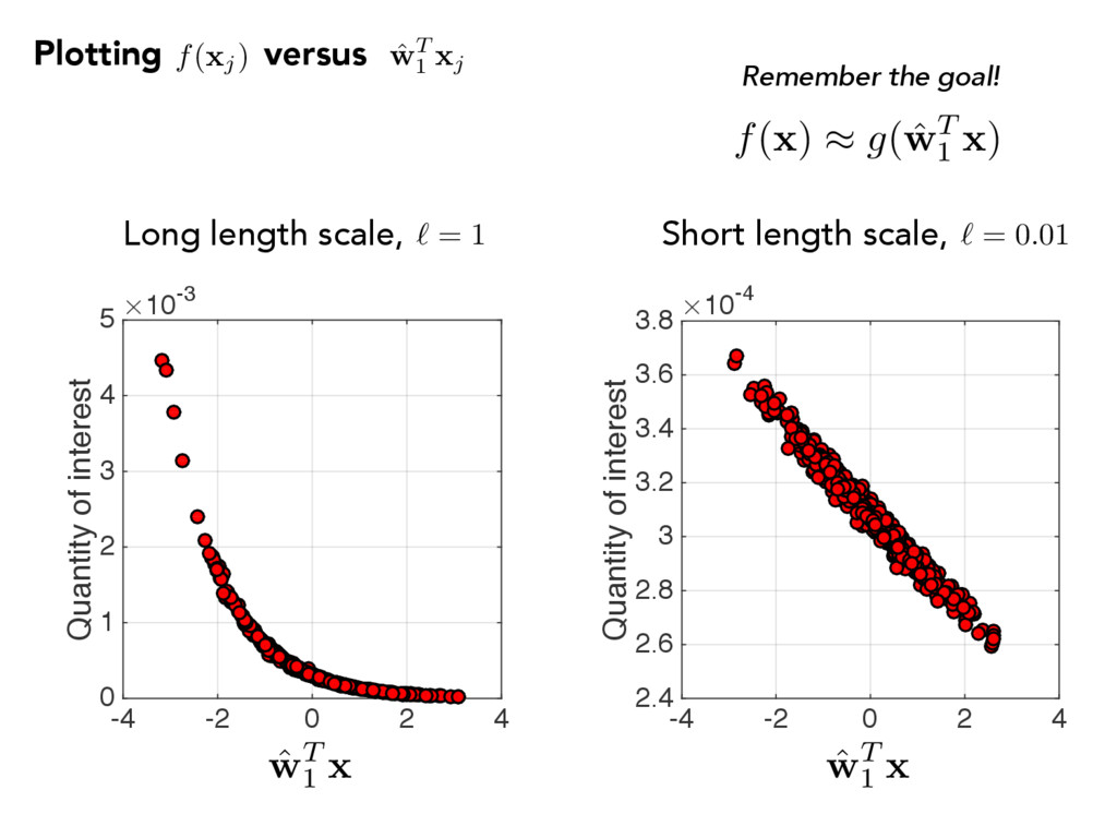
1 2 3 4 5 -4 -2 0 2 4 Quantity of interest #10-4 2.4 2.6 2.8 3 3.2 3.4 3.6 3.8 Long length scale, ` = 1 Short length scale, ` = 0.01 f( x ) ⇡ g( ˆ w T 1 x ) ˆ w T 1 x ˆ w T 1 x Remember the goal! Plotting versus f( xj) ˆ w T 1 xj
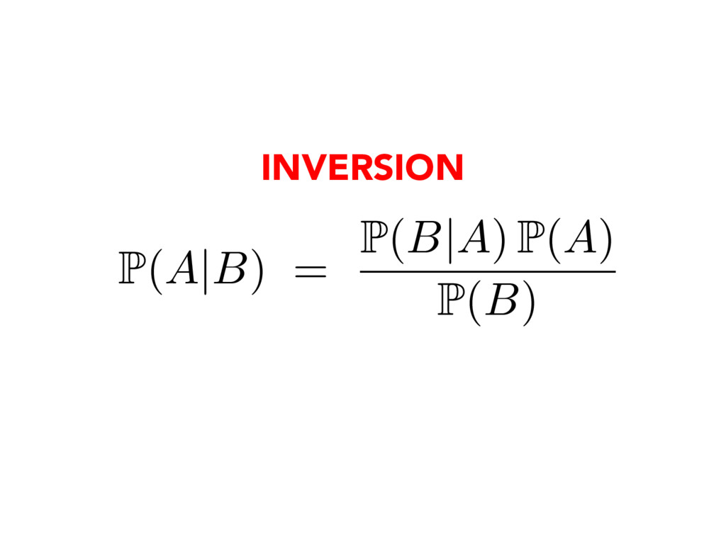
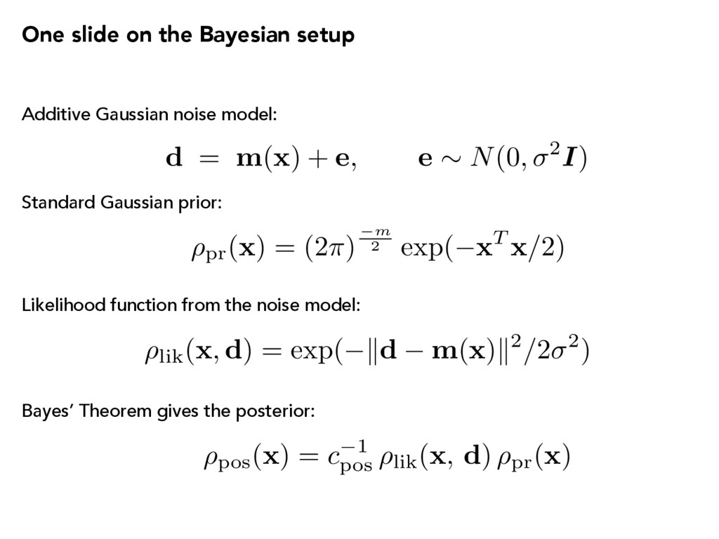
⇠ N(0, 2I) ⇢lik(x , d) = exp( k d m(x) k2/ 2 2 ) ⇢ pos ( x ) = c 1 pos ⇢ lik ( x , d ) ⇢ pr ( x ) One slide on the Bayesian setup Additive Gaussian noise model: Standard Gaussian prior: Likelihood function from the noise model: Bayes’ Theorem gives the posterior: ⇢pr(x) = (2 ⇡ ) m 2 exp( x T x / 2)
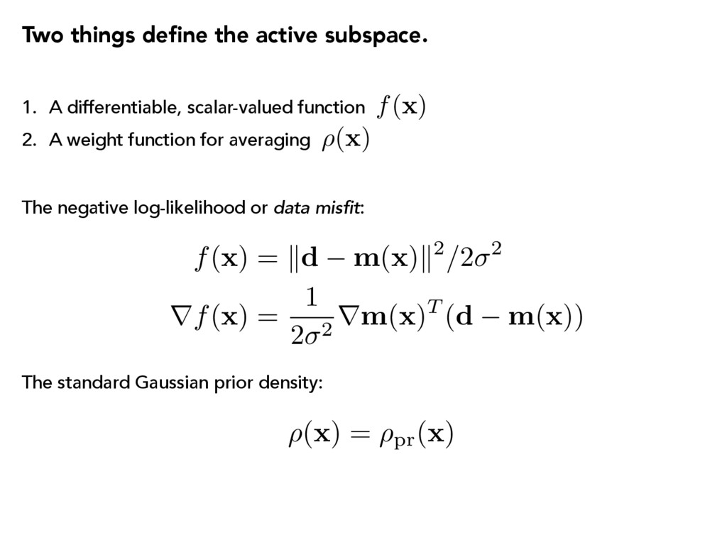
2 rf( x ) = 1 2 2 r m ( x )T ( d m ( x )) 1. A differentiable, scalar-valued function 2. A weight function for averaging Two things define the active subspace. ⇢( x ) f( x ) The negative log-likelihood or data misfit: The standard Gaussian prior density: ⇢( x ) = ⇢pr( x )
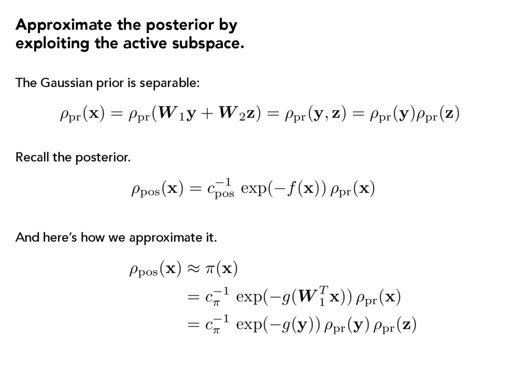
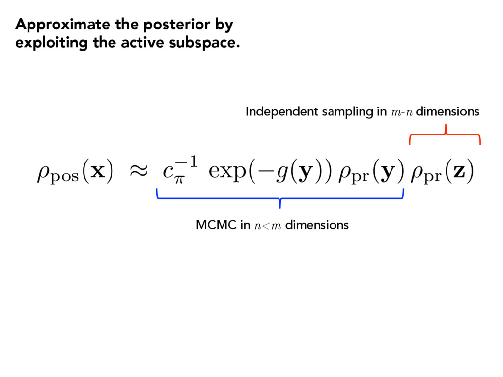
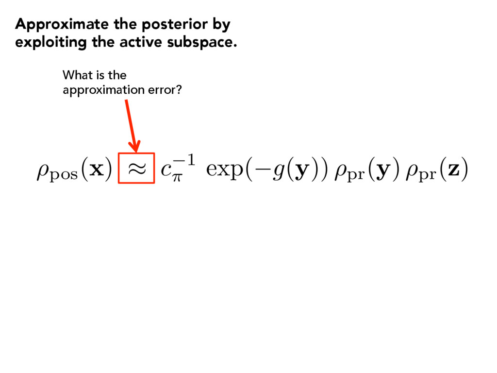
pr(x) ⇢ pos(x) ⇡ ⇡ (x) = c 1 ⇡ exp( g ( W T 1 x)) ⇢ pr(x) = c 1 ⇡ exp( g (y)) ⇢ pr(y) ⇢ pr(z) ⇢pr( x ) = ⇢pr(W 1y + W 2z ) = ⇢pr( y , z ) = ⇢pr( y )⇢pr( z ) Approximate the posterior by exploiting the active subspace. The Gaussian prior is separable: Recall the posterior. And here’s how we approximate it.
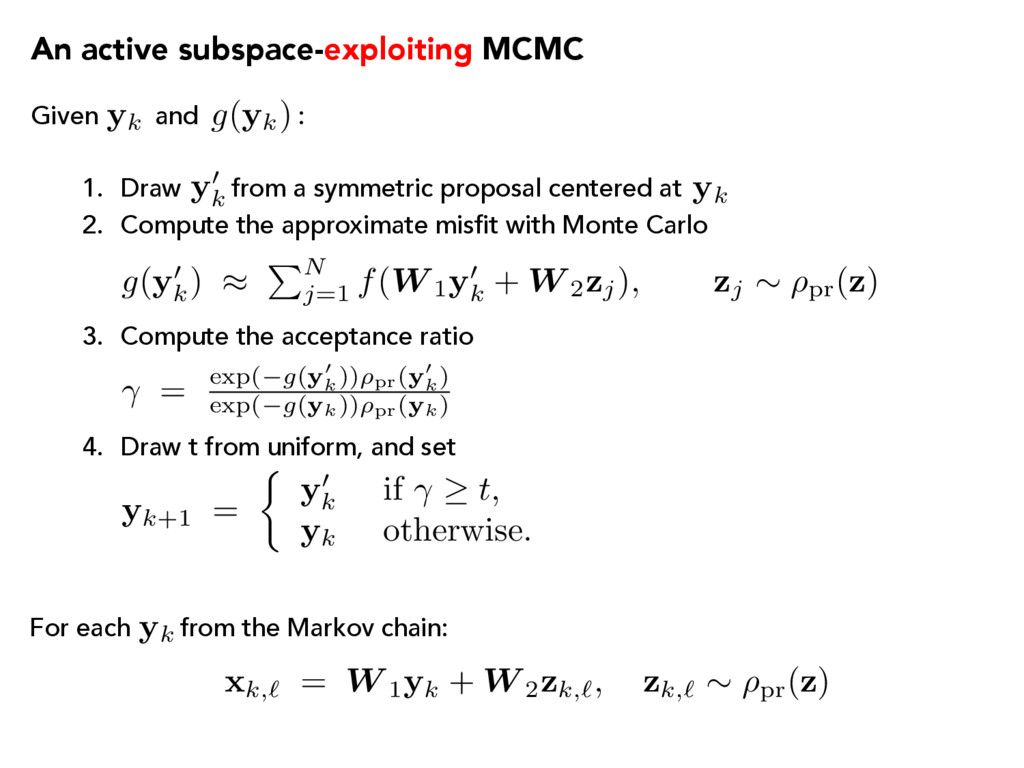
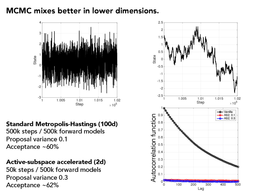
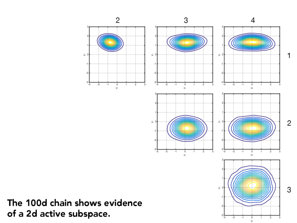
a symmetric proposal centered at 2. Compute the approximate misfit with Monte Carlo 3. Compute the acceptance ratio 4. Draw t from uniform, and set yk y0 k yk g(y0 k ) ⇡ PN j=1 f(W 1y0 k + W 2zj), zj ⇠ ⇢pr(z) g(yk) = exp( g ( y0 k)) ⇢pr( y0 k) exp( g ( yk)) ⇢pr( yk) yk+1 = ⇢ y0 k if t , yk otherwise. yk For each from the Markov chain: xk,` = W 1yk + W 2zk,`, zk,` ⇠ ⇢pr( z )
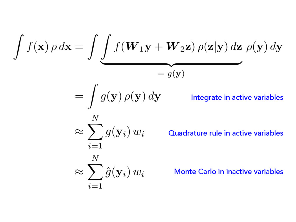
f(W 1y + W 2z ) ⇢( z | y ) d z | {z } = g(y) ⇢( y ) d y = Z g( y ) ⇢( y ) d y ⇡ N X i=1 g( yi) wi ⇡ N X i=1 ˆ g( yi) wi Integrate in active variables Quadrature rule in active variables Monte Carlo in inactive variables
What if I don’t have gradients? • What kinds of models does this work on? • Can you show some applications? • What about multiple quantities of interest? • Tell me about hypercubes. • How new is all this? PAUL CONSTANTINE Ben L. Fryrear Assistant Professor Colorado School of Mines activesubspaces.org! @DrPaulynomial! QUESTIONS?
![[ Show them the MATLAB demo! ]](https://files.speakerdeck.com/presentations/80d62cbdf81b41278210e8ff18ce1528/slide_46.jpg)
![• How do active subspaces relate to [insert method]? •](https://files.speakerdeck.com/presentations/80d62cbdf81b41278210e8ff18ce1528/slide_56.jpg)