Upgrade to Pro — share decks privately, control downloads, hide ads and more …

p-values Role in Modern Social Science Research

Dr.Pohlig
April 04, 2014

p-values Role in Modern Social Science Research

p-values Role in Modern Social Science Research
Given April 4, 2014, @ the University of Scranton

*For those who don't know: Baril & Cannon (from the Bayes, Baril, & Cannon slides) were two of my prof's at Scranton.

Dr.Pohlig

April 04, 2014
Tweet

More Decks by Dr.Pohlig

Other Decks in Research

Transcript

  1. RYAN T. POHLIG BIOSTATISTICIAN COLLEGE OF HEALTH SCIENCES, UNIVERSITY OF

    DELAWARE U OF S CLASS OF 2005 THE REPORT OF MY DEATH WAS AN EXAGGERATION: P-VALUES’ ROLE IN MODERN SOCIAL SCIENCE RESEARCH
  2. Recently, poorly conducted research has become a “hot topic” in

    the Social and Health Sciences. Attempts to move these fields into more rigorous scientific directions have criticized the standard practice of reporting p- values. This talk will cover a few ways that researchers should be aware of for manipulating p-values, and how to avoid making these (sometimes inadvertent) errors in your own work.
  3. Criticizing p-values Cumming, G. (2014). There’s life beyond .05: Embracing

    the new statistics. Observer 27, 19-21. Retrieved from https://www.psychologicalscience.org/index.php/publications/observer/2014/march-14/theres- life-beyond-05.html Nuzzo, R. (2014). Statistical Errors: P values, the ‘gold standard’ of statistical validity, are not as reliable as many scientists assume. Nature 506, 150-152 Retrieved from http://www.nature.com/polopoly_fs/1.14700!/menu/main/topColumns/topLeftColumn/pdf/506 150a.pdf Kurzban, R. (2013)P-hacking and replication crisis. Edge.org Retrieved from http://edge.org/panel/robert-kurzban-p-hacking-and-the-replication-crisis-headcon-13-part-iv Ziliak, S. T. (2013). Unsignificant Statistics. Financial Post. Retrieved from http://opinion.financialpost.com/2013/06/10/junk-science-week-unsignificant-statistics/ Lambdin, C. (2012). Significance tests as sorcery: Science is empirical- significance tests are not. Theory & Psychology 22, 67-90. Retrieved from http://psychology.okstate.edu/faculty/jgrice/psyc5314/SignificanceSorceryLambdin2012.pdf Simmons, J. P., Nelson, L. D., & Simonsohn, U. (2011). False-positive psychology: Undisclosed flexibility in data collection and analysis allows presenting anything as significant. Retrieved from http://people.psych.cornell.edu/~jec7/pcd%20pubs/simmonsetal11.pdf APS Observer, March 2014
  4. In the media “Therefore, to publish a paper in a

    scientific journal, appropriate statistical test are required. Researchers use a variety of statistical calculations to decide whether differences between groups are statistically significant- real or merely a result of chance. The level of significance must also be reported. Results are commonly reported as statistically significant at the 0.05 level. This means that it is 95 percent certain that the observed difference between groups or sets of samples, is real and could not have arisen by chance.” Bold is author’s original emphasis ◦ Sherry Seethaler, 1/23/09, in “Lies, Damned Lies, and Science: How to Sort through the Noise Around Global Warming, the Latest Health Craze, and Other Scientific Controversies”
  5. In the media 2 “This number (the p stands for

    probability) is arrived at through a complex calculation designed to quantify the probability that the results of an experiment were not due to chance. The possibility of a random result can never be completely eliminated, but for medical researchers the p-value is the accepted measure of whether the drug or procedure under study is having an effect. By convention, a p-value higher than 0.05 usually indicates that the results of the study, however good or bad, were probably due only to chance.” ◦ Nicholas Bakalar, 3/11/13, NY Times “Putting a Value to ‘Real’ in Medical Research”
  6. In the media 3 p-value is the “probability that you

    see this effect by chance alone” ◦ Charles Seife, 6/23/12, author of “Proofiness: The Dark Arts of Mathematical Deception” during his Authors@google talk. These quotes are a fairly accurate portrayal of how p-values are defined or described as in the media and in “popular” books What did you write down?
  7. Defined What is a p-value? 1. It is a “probability”

    2. It is an “area” not a point, it is probability of obtaining the results seen, or ones more extreme 3. It is the probability of obtaining the results seen or ones more extreme, given the Null Hypothesis is true 4. It is probability of obtaining the results seen or ones more extreme, given the Null Hypothesis is true, due to Random/Sampling Error and ONLY Random/Sampling error Technically, a p-value does not give probability the result was due to chance but it indicates whether the results are consistent with being due to chance. *H0 means no effect, no relationship
  8. p-value components Three concepts in a p-value 1. Probability ◦

    Number of Outcomes classified as an event over total possible outcomes ◦ Technically, it is an area, which is a set of events over total possible outcomes 2. If the Null Hypothesis is true ◦ If null is true, there is no effect or relationship 3. Due to sampling error ◦ When testing significance, we test an effect by taking an estimate relative to ◦ standard error ◦ Mean difference in t-test ◦ Amounts of variation due to effects in an ANOVA ◦ Slope estimate in regression ◦ The standard error is the standard deviation of the sampling distribution ◦ Sampling distribution is the distribution of a statistic that is created by taking all possible random samples of a given size (n)
  9. Use for p-values: A Quick Null Hypothesis Testing Review p-values

    can be adopted for use in Null Hypothesis Testing. The Null Hypothesis (H0 ) states that in the population, there is no effect (there is no difference or no relationship). The Alternative Hypothesis (H1 or HA ) states that there is an effect (there is a difference or relationship in the population). The Null Hypothesis and the Alternative Hypothesis are mutually exclusive and exhaustive. •They cannot both be true. •They need to cover all potential outcomes.
  10. A Type I, α, error occurs when a researcher rejects

    a null hypothesis that is actually true. A Type II, β, error occurs when a researcher fails to reject a null hypothesis that is actually false. Conclusions reached in NHT
  11. The concepts of Null Hypothesis Testing come from a different

    framework than p-values. ◦ R. A. Fisher developed p-values ◦ J. Neyman - E. Pearson developed Null vs Alternative Hypothesis testing ◦ Pick an acceptable error rate. ◦ Use the error rate to find a critical statistic that an observed value beyond would be “significant” ◦ Compare your observed results to your error rate and decide if your findings were worth mentioning ◦ Critical statistic is based off distributional assumptions (n/df, standard deviation/variance,…) These approaches have been blended together, for better or worse ◦ Some statisticians think they are incompatible ◦ This is a whole separate presentation History
  12. .05 By convention we set alpha to be .05, and

    this has been adopted as industry standard for most social and health research. But Why? Got me The quote most people eventually fall back on is from R. A. Fisher in “Statistical Methods for Research Workers” (first edition 1925) ◦ “The value for which P = .05, or 1 in 20, is 1.96 or nearly 2; it is convenient to take this point as a limit in judging whether a deviation is to be considered significant or not. Deviations exceeding twice the standard deviation are thus formally regarded as significant.” Yet in the same text: ◦ “If one in twenty does not seem high enough odds, we may, if we prefer it, draw the line at one in fifty (the 2 percent point), or one in a hundred (the 1 percent point). Personally, the writer prefers to set a low standard of significance at the 5 per cent. point, and ignore entirely all results which fail to reach this level. A scientific fact should be regarded as experimentally established only if a properly designed experiment rarely fails to give this level of significance.”
  13. p-values Are Misunderstood 1. p-values do not indicate a “degree

    of significance”. ◦ A smaller p-value does not mean the results are stronger or the effect was larger. 2. There is no such thing as Marginal Significance, or Trending Towards Significance. ◦ If your p-value is above you’re a priori alpha level, the treatment did not work or relationship was not significant. 3. p-values are not probabilities about alternative hypotheses. ◦ They are probabilities about a specific data’s null hypothesis ◦ A Bayesian method, specifying priors and employing a likelihood function would be needed.
  14. 4. pobs ≠ αobs ◦ An observed p-value is not

    a sample/statistical test’s specific Type-I error rate. ◦ It is incorrect to conclude that your observed p-value, is the probability that your results are a type-I error. ◦ If your p = .034, you CANNOT say that there is a 3.4% chance of concluding there is an effect when there is not. ◦ This flows from the distinction between the two different frameworks, and I think confusion arises as both p and α are tail probabilities ◦ It is impossible to observe a type-I error rate from one result. ◦ Key difference is that α is based on repeated random sampling from a well defined population ◦ α is the long-run relative frequency of Type I errors conditional on the null being true Misconceptions part 2
  15. Misconceptions part 3 5. Α When you combine misunderstandings 3

    & 4, you get the “Fallacy of the Transposed Conditional” ◦ P(Data|H0 =true) ≠ P(H0 =true|Data) ◦ p-value is not the probability of null being true given the result of the data, but the probability of the data yielding the result given the null is true, p-value = P(Data|H0 =true)
  16. Practical issue of using p-values in conjunction with NHT. ◦

    If something is significant- it must be worth publishing! ◦ This dichotomous thinking, creates bias ◦ You results are “significant” or “not significant” Publication Bias is the difference between what is likely to be published versus what could be published. ◦ If research that was unpublished was random there wouldn’t be a problem. ◦ Publication bias can be a positive thing. For instance a bias against publishing studies that used knowingly fabricated data is a good thing. A specific case of publication bias might be familiar to you, the “File Drawer Problem” ◦ What types of studies tend to get published? Implicitly we know there may be a bias towards research with significant findings over those with null-results (negative findings). A step further- The Circular File problem ◦ This is when non-significant studies are not even put in the file drawer but placed directly into the trash, creating the problem of having no idea how many studies even failed. Biasing Research
  17. Publication bias A meta-analysis of meta-analyses examining Clinical Trials was

    performed in 2009 by Hopewell, et al. to look at publication bias. ◦ There were 5 meta-analyses examined (750 articles) ◦ Clinical trials with positive findings were almost 4x more likely to be published than trials with negative or null findings (OR = 3.90) ◦ Also found that studies with positive findings were quicker to be published (4.5 years compared to 7 years) ◦ Sex of first author, investigator rank, size of trial, and source of funding had no effect Similarly, Song et al. (2009) ran a meta-analysis on cohort studies ◦ Found that positive results were about 3x more likely to be published (OR = 2.78) If null-findings are not published how often are resources (money, time, opportunities…) wasted researching someone else has found already to not work?
  18. Additional Consequences of .05 The arbitrariness of .05, and “significance”

    has created other problems, particularly at the researcher level. Now there is a target for researchers to hit, and hitting it means they have found something “significant” - this could lead to manipulation of results. Is there evidence of manipulation? Masicampo & Lalande (2012) examined 3 psych journals, and tabulated the distributions of the p-values reported. ◦ Journal of Experimental Psychology: General ◦ Journal of Personality and Social Psychology ◦ Psychological Science ◦ Looked at all articles in the journals from July ‘07 to Aug ‘08 Found that values just below .05, where higher than what would be expected.
  19. Arbitrariness The number of observed p-values are higher right near

    the cut point of .05. Here it is presented at four different “bin” sizes. You can see the bump right by .05.
  20. Manipulation cont. Leggett, Thomas, Loetscher, and Nicholls (2013), compared 2

    journals for 2 different years [1965 and 2005], to examine if this trend was increasing over time. ◦ Journal of Experimental Psychology: General ◦ Journal of Personality and Social Psychology Found that values just below .05, where higher than what would be expected, and this increase was greater in 2005 than 1965.
  21. On the left are the numbers for the JPEG, on

    the right are JPSP. Top and bottom re different bin sizes. The triangles are 2005, and circles are 1965. We can see that same bump right by .05. Arbitrariness
  22. The push to publish was posited as a reason for

    the difference between the years Arbitrariness
  23. Comparing Sciences The softer sciences tend to publish “significant” results

    more often than other fields. Fanelli (2010) examined if the publication bias differed by field- and found that as you get more and more behavioral there was a higher percentage of publications reporting significant effects.
  24. Magical “.05” Mark & Bias Created in the Methods TYPE-I

    ERROR INFLATION via Multiple Comparisons, Independence, & Sample Size
  25. Blaming p is trendy, but is it correct? Another consequence

    of the having this target, is researchers may modify studies, analyses, and protocols to try and find significance ◦ They know their data has truths that need to be uncovered. ◦ [Completely anecdotal but] I find that researchers come to me asking how they should look at their data, only to find they have already tried and failed to find something significant. A major problem is “Type-I error Inflation” ◦ Importantly, it should be noted that this is not a problem with p-values but a problem with research practices. ◦ The more statistical tests you run on a set of data the higher the probability of making a type-I error. One way researchers inflate Type- I errors AND increase their chance of finding significance is by examining their data over and over again. ◦ These “Multiple Comparisons” are not always wrong. ◦ Often research deals with complex phenomena where many different hypothesis are evaluated simultaneously ◦ Post-hoc multiple comparisons are needed for many GLM & GLMM models
  26. Multiple Comparisons For instance making 10 comparisons with the same

    data with α = .05 for each comparison. This results in an overall α being much higher ◦ in this case α’ = .4. ◦ α’ = 1-(1- α)k, where k is number of comparisons to be made. ◦ Abdi (2007) in a simulation study found with just 5 comparisons at .05, the type-I error rate was .21 which is close to the formulas' estimate of .226 One example, Cacioppo et al. (2013) published a study “Marital satisfaction and break-ups differ across on-line and off-line meeting venues” included more than 19,000. ◦ I stopped counting significance tests at 74 and there were 3 other appendix tables, I did not count.
  27. Multiple Comparisons part 2 Avoid “Shotgun Studies” ◦ Have more

    outcomes than seems reasonable ◦ Recently a researcher asked me to compare pre and post measures on 10 different outcomes with a sample of 15 individuals. ◦ This is essentially a priori Data Mining, has been called data diving, data dredging, or p-hacking ◦ Data mining techniques should be used, and disclose that this is what was done. Many predictors or independent variables with no strong research/experimental hypothesis ◦ Use automated model selection procedures to reduce chance of type I error ◦ Can also use “penalty functions” Large numbers of covariates or dependent variables ◦ Use multivariate statistics when possible to avoid inflating type I error ◦ If “confirmatory” use SEM ◦ If exploratory can try to reduce the number of variables by using a data reduction techniques ◦ like PCA or calculating a risk score
  28. Multiple Comparisons part 3 Post-hoc narrowing your sample to a

    specific sub-group. ◦ This includes eliminating some individuals as well as separating groups out. ◦ “Well, the literature tells us it only works for people who are X, Y, & Z.” ◦ Also have now changed your target population you powered your study off and wanted to generalize too. Post-hoc narrowing your instrument to certain questions. ◦ “We found no significance when looking at total score. But items 2 and 3 really address our construct of interest” ◦ If instrument had previous research supporting its use, that validity evidence is now gone.
  29. Handling Multiple Comparisons Have to adjust for multiple comparisons no

    if’s, and’s, or but’s. ◦ There is an argument for not adjusting for some a prior comparisons. ◦ The downside in controlling for multiple comparisons is to be more conservative. ◦ When comparing groups or running many outcome variables there are a variety of ways to do this: ◦ Adjustments (Bonferonni’s, Sheffe, Sidak, etc.), Estimating False Discovery Rates, Resampling methods ◦ If you are doing something akin to data-mining and the adjustments (Bonferonni et al.) set α at an unobservable level, then use a more conservative alpha throughout, i.e. α =.001. ◦ If you want to test if there is bias for each item on a 55 item test If you know a priori you will have multiple comparisons you should power your study with this in mind. ◦ Calculate sample size or effect size after reducing alpha. If you want to create and validate a model using one data set, you should randomly split the data file into multiple parts, use the first part to build your model and the second to validate it.
  30. Assumption of Independence Violating the assumption of Independence ◦ A

    type of systematic error, that is caused by flawed research designs and poorly chosen analysis. Independence is the one assumption that is required of all statistical tests at some level. ◦ Might be independence of subjects, independence of measurement occasions, conditional independence, independence of disturbances, or independence at highest level of nesting/clustering Not accounting for the lack of independence will cause bias in p-values ◦ Using between subject analyses on data from with-in subject/repeated measure designs. ◦ Having nested or clustered factors and ignoring it. Cacioppo et al.’s Marital satisfaction study did not look into adjusting estimates if they ended up measuring both individuals in a relationship. Multilevel modeling should be employed (when possible given n size). ◦ Not accounting for independence can inflate a type I error rate from .05 up to .80 (Aarts, et al., 2014)
  31. Type-I error by Cluster Size by ICC size Intraclass Correlation

    Coefficient (ICC) is a measure of how much variability is accounted for by clustering or nesting ICC = .5 ICC = .1 Type-I error when using MLM for both ICC = .5 and ICC = .1 Not Accounting for nesting
  32. Under [and Over] Powered Authors will claim with an increase

    in sample size you would increase power, and be able to find significance. This is true. Think about its implications though ◦ Every study that ever existed that was not-significant was/is “underpowered” ◦ Given that relationship or mean difference wasn't exactly 0 . ◦ You can in theory continue to increase your n to make any size effect significant. Finding very minute differences or tiny relationships statistically significant does not mean there is any real value (or significance) there. ◦ At this point the study has become “over-powered.” Two other common practices ◦ Turning study data into a pilot, “We didn’t quite get significance in this pilot study, with a larger n we will be able to detect this effect.” ◦ Turning pilot data into a study- “The Growing n” idea ◦ Continue to increase sample until significance is reached Always mention how the “n” size you used was arrived at, if you ran a power analysis mention the effect size you were aiming to find.
  33. p is the Wrong Target We should expect at least

    5% of all published research to be a type-I error due to random-sampling error. ◦ This should be forgivable- it is built in to the way scientific research functions ◦ Not all errors are poor methodology or result of bad design If the research is flawed, the use of p-values is irrelevant ◦ The study design was flawed ◦ Implementation was improper ◦ Researcher bias (i.e. not blind or double blind, Hawthorne effect…) ◦ Wrong statistical analysis was done ◦ Statistical Assumptions violated and ignored, etc. Most examples where the conclusion of a significant effect or relationship was reached in error was caused by some sort of Systematic Error NOT Random Error.
  34. Ethically Analyzing Data It is very easy to convince ourselves

    that these practices are not unethical and in fact depending upon the circumstances they might appropriate or even recommend. Researchers might not even realize what they are doing may be unethical. My stance that you should be forthright and disclose any and all data manipulations or changes that occurred. An investigators Research Question (RQ) should always drive the design, and analysis that is chosen. ◦ It will dictate what are your, Independent Variables (IV), Dependent Variables (DV), and Covariates (CVs) Changing your variables and/or model without cause ◦ Categorize a continuous variable or combine levels
  35. Ethics part 2 Adding covariates post-hoc, without explanation ◦ Should

    have a substantive reason to include a variable as a covariate ◦ Even if it is to just reduce error variance, you should mention that is the reason Always disclose if you ◦ Dropped conditions or variables ◦ Added conditions or variables Changing from repeated measures design and analysis to independent samples without disclosing why the change. Post-hoc narrowing your instrument to certain questions, whether it is the IV or DV. ◦ “No significance in total score but items 2 and 3 are really address our construct of interest” ◦ If instrument had previous research giving it validity evidence, you have now lost that support
  36. During Analysis If you have problems with your data, run

    analyses before and after fixing them, to see if they changed the result. Report all attempts at finding same effect. ◦ This will inform consumers about your research and any potential file-drawer or circular-file problems Never HARK ◦ Hypothesizing After Results are Known Do not change observed data ◦ Can be tempting if study is not double blind ◦ More common than you think as researchers always say, “I know how she/he meant to respond…”
  37. Assumption Checking Assumptions [talk in its own right] ◦ Every

    statistical test you will ever use has a set of assumptions ◦ ALWAYS check assumptions ◦ In order to draw accurate conclusions, you must satisfy the assumptions (or cite research showing that the method is robust to its violation) ◦ Report any assumptions you violated, and the remedies you used ◦ Always disclose that you ◦ Excluded outliers ◦ Included potential outliers
  38. Transformations Applying transformations ◦ This can help with outliers ◦

    Transformations do not change the relative standing of the data on a variable ◦ What they change is the variability in the data ◦ If you are going to perform a transformation I recommend using the Box-Cox test ◦ Will tell you if a model is not linear, presence of non-linearity is an indicator of non-normality ◦ Will also supply which transformation is the one that will fix it best ◦ Care should be taken when manipulating the data by transforming it ◦ Never apply transformations without mentioning it, transforming data alters interpretation of results as the variables are now different ◦ Run analysis and either report or mention you have results with and without transformations
  39. Missing Data Missing data [Another talk in its own right]

    ◦ Disclose the amount and maybe the patterns ◦ Do not listwise delete (remove all cases for all analysis) without disclosing why Should look for “missingness” patterns ◦ Missing Completely at Random (MCAR) ◦ Will not cause bias, the only type of missingness you want ◦ Missing at Random (MAR) ◦ May cause bias in estimates ◦ Missing Not at Random (MNAR ) ◦ Will cause bias in estimates Do not impute data without stating specifically the method you chose ◦ Mean imputation reduces variability, introduces bias ◦ Regression imputation reduces error variance, and introduces bias ◦ Expectation-Maximization (EM), the only one I can partially recommend but even then it can introduce bias
  40. Requires meta-analytic solutions ◦ Thus it can only be used

    when investigating effects aggregating over studies ◦ Can be 5-10 years before a meta- analysis performed Two suggestions are using “Funnel Plots” and trying to estimate the number of studies that have been stuffed into the drawer. Funnel Plot ◦ A scatter plot that looks at effect by study size ◦ If no publication bias, there should be no visible relationship between effect and study size, other than a “funneling” Trying to Detecting Publication Bias
  41. Meta-Analysis in One Slide Each box is a point estimate

    from an article. The bars extended from them are their corresponding confidence intervals. The benefit or strength of a Meta- Analysis is the ability to take all of these results and combine them to get a better estimate of the true effect. ◦ Here that would be a -.33 correlation
  42. Detecting Publication Bias Ideally, using funnel graphs would result in

    the images below ◦ The first graph shows no evidence of bias ◦ The right graph shows that small study sizes are not detecting large effects…
  43. Fix the hole You could then “remove” bias by imputing

    results that were missing by using “trim & fill” ◦ No universal recommendation on a fill method ◦ Imputing missing effects to reduce bias could introduce more bias by assuming all missing follow same pattern Does it work? ◦ Unfortunately, a simulation study was performed testing the ability of researchers to use funnel plots and found them to be wanting. ◦ Researchers had 53% accuracy in finding if there was a “hole”… (Lau, Ioannidis, & Olkin 2009) ◦ But if they do find it accruately, the “fill” part has some evidence to support it (Duval & Tweedle, 2000).
  44. Fail-Safe File-drawer The fail-safe file-drawer method was proffered to try

    and evaluate if file- drawer problem is causing spurious results. ◦ You estimate the number of studies needed to be added to a meta-analysis to eliminate the effect seen (cause p ≤ α). ◦ If the “fail-safe” number is extremely large relative to the observed number of studies, it is concluded that the effect is likely ◦ If you have 50 studies in the meta-analysis and it would take 5000 unpublished studies to eliminate the effect ◦ Number of different ways to calculate, and they give vastly different results ◦ “This method incorrectly treats the file drawer as unbiased and almost always misestimates the seriousness of publication bias… Statistical combination can be trusted only if it is known with certainty that all studies that have been carried out are included. Such certainty is virtually impossible to achieve in literature surveys.” (Scragle, 2000)
  45. Killeen (2005) proposed prep to “estimates the probability of replicating

    an effect” There are a few problems with this idea 1. It is based only off information from the p-observed, a one to one correspondence ◦ No new information is added 2. Unfortunately, the math didn’t hold up 3. Lastly, the statistic is based on a single sample’s observation, and encounters a flaw in its reasoning. It would be the probability of replicating the results given the same exact sample, in the same circumstances… ◦ The idea of replication is to account for unmeasured factors in the testing environment, unmeasured participant variables, response biases, investigator effects and to see if the findings occur with a different sample of participants. prep
  46. Confidence Intervals It has been suggested that reporting Confidence intervals

    would be an appropriate solution. What is a CI? ◦ Point Estimate is the sample statistic estimated for the population parameter of interest. ◦ Critical Value is a value based on the desired confidence level. ◦ A typical confidence level is 95%. Also written as 1 - α = 0.95, here α = 0.05. ◦ Standard Error is the standard deviation of the point estimate’s sampling distribution A confidence level (e.g., 95%) is the probability that the 95% CI will capture the true parameter value in repeated sampling. ◦ 95% of all the confidence intervals of size n that can be constructed will contain the true parameter. Point Estimate ± (Critical Value)(Standard Error)
  47. Confidence Intervals part 2 CI’s are a more concise way

    of indicating the result of a significance test, the point and variability estimates. Confidence intervals are built using the critical value that is chosen based on α. ◦ Your CI will always give you the SAME exact conclusion the p-value does. ◦ If you report descriptive statistics then the CI interval adds nothing. ◦ This is not a solution to the p-value “problem.” Confidence Intervals Sample 1 Sample 2 Sample 8 True parameter value
  48. Bayesian Methods Bayes, and Bayesian Statistics are a whole talk

    in their own right. Recall that a p-value is the P(Data|H0 =true) and is not ≠ P(H0 =true|Data). You can use Bayes Theorem to estimate P(H0 =true|Data). Conceptually Bayesian thinking and methods add a factor of “Plausibility” ◦ Before you start your research you estimate how plausible (or probable) you think the outcome is, whether it is a mean difference or relationships among variables. ◦ This is called the prior, and is P(B) ◦ After running your study you adjust your results by including the prior ◦ By doing so you end up with a posterior probability. ◦ p(A) is a normalizing constant, that is the marginal distribution, sometimes referred to as prior-predictive distribution
  49. “Why Most Published Research Findings are False” Ioannidis (2005) applied

    Bayesian thinking [and Bayes theorem] to estimate the “positive predictive value” (PPV) or research findings. PPV can conceptually be thought of as the probability of finding an effect if an effect exists. He generalized the concepts of α, β, and power by taking them over a population of hypothesis and put them in the framework of epidemiology using sensitivity, specificity, and (predictive power). ◦ Have to assuming the “prior” (odds that an effect exists) ◦ This idea lets you include another factor, either assuming or estimating it (like bias or the number of people investigating a phenomena). ◦ Also need to assume or fix “power” to use. With a few assumptions we are able to calculate the impact of a variety of factors.
  50. PPV TRADITIONAL NHT True False Exists Does not Observed Exists

    1-β α Does not β 1-α IN POPULATION True False Exists Does not Observed Exists 1-β α Does not β 1-α Total c 1-c β = probability of finding no relationship when one exists. α = probability of finding a relationship when one does not exist 1-β = power, finding a relationship that does exist c = proportion of true hypotheses 1-β = sensitivity 1-α = specificity
  51. PPV part 2 True False Exists Does not Observed Exists

    1-β α Does not β 1-α Total c 1-c Now we do a calculation that is just like finding out the probability of you having a disease, given you tested positive- and the test has known sensitivity and specificity rates. ◦ PPV = ratio of hits to all positives = c(1-β)/{c(1-β)+(1-c)α} ◦ correct findings = c(1-β) = number of true*power ◦ false positives = (1-c)α = number of non-true*faulty finding rate c = proportion of true hypotheses 1-β = sensitivity 1-α = specificity
  52. PPV extended for bias True False Exists Does not Observed

    Exists 1-β+uβ α + u(1-α) Does not (1-u)β (1-u)1-α Total c 1-c Now you can incorporate a bias estimate ◦ PPV = ratio of hits to all positives = c(1-β+uβ)/{c(1-β+uβ)+(1-c) [α + u(1-α)]} ◦ correct findings = c(1-β) = number of true*power ◦ false positives = (1-c)α = number of non-true*faulty finding rate c = proportion of true hypotheses 1-β = sensitivity 1-α = specificity u= proportion due to bias
  53. PPV extended for investigators True False Exists Does not Observed

    Exists 1-βn 1-(1-α) n Does not βn (1-α) n Total c 1-c Now you can incorporate for multiple investigators ◦ PPV = ratio of hits to all positives = c(1-βn)/{c(1-βn)+(1-c) [1-(1-α) n]} ◦ correct findings = c(1-β) = number of true*power ◦ false positives = (1-c)α = number of non-true*faulty finding rate c = proportion of true hypotheses 1-β = sensitivity 1-α = specificity n = number of investigators
  54. Ioannidis (2005) part 2 Resulting from his idea are a

    number of corollaries. 1. The smaller the n, less likely research is true. 2. The smaller the effect sizes, less likely research is true. 3. The larger the number of relationships tested, the less likely to be true. ◦ Hunting for significance 4. The greater the “flexibility” of designs, analyses, definitions the less likely to be true. ◦ Randomized controlled trials > observational studies 5. Greater the financial interest the less likely to be true. 6. Paradoxically, the more people investigating a phenomena the less likely it is to be true. ◦ The more people investigating the more prevalent null findings become.
  55. Bayesian Alternatives Use a “Bayes Factor” which is analogous to

    significance testing in a Bayesian framework. ◦ One advantage is that it can help choose among competing models ◦ Another advantage is that they are more robust than p-values ◦ Requires the same arbitrary cut-off for something being deemed important, type I and type II errors still exist. ◦ Can be unstable, and when used in complicated models the prior can become very influential Use a Bayesian “Credibility Interval”, which is an interval in the posterior probability distribution. ◦ These are interpretable as what most want to say for Confidence intervals. ◦ Have to use a sensitivity analysis to determine impact of the prior ◦ Can be difficult for complex models
  56. Bayesian Alternatives part 2 Empirical Bayes methods is like a

    combination of Bayesian and traditional methods. ◦ Priors are calculated using the observed data. ◦ Have both parametric and non-parametric approaches Other suggestions include using likelihood ratio, and a full Bayesian analysis which can eliminate much of the uncertainty in estimation. ◦ Limited to only a few or no nuisance parameters ◦ Difficult for complex designs ◦ Often the likelihood ratio threshold is equivalent to a p-value threshold ◦ Requires a model to start with, if no statistical model exists it can not be done
  57. Bayes, Baril & Cannon Cohen (1994) wrote The Earth Is

    Round (p<.05), discussing some of the short comings of using p-values, primarily mentioning the Fallacy of the Transposed Conditional. Cohen’s argument was that you can use Bayes Theorem to show how different the two conditional probabilities are. ◦ To illustrate his point he used strong priors [quite large values], i.e. 98% likelihood the null is true ◦ Did the math and showed that misinterpreting the p-value can lead to a false sense of strong evidence against the null. Dr’s Baril and Cannon (1995) pointed out that this was true in his examples because of using the unrealistic priors ◦ These were causing the large differences in the two conditional probabilities ◦ Reran the numbers using less strong priors, explaining why weaker priors made more sense in the real world explaining that small effects are less likely to be true. ◦ They decided to use Cohen’s d, anything under a “small effect”( < .2), would be evidence of the null being true. ◦ They found the proportion of data that had less than the small effect sizes and used that as their prior.
  58. What did Baril & Cannon find? ◦ Did so and

    found the two to be quite similar (.016 to .05), and in fact conservative, if the probability of the null hypothesis was true was not extreme, .16. ◦ By necessity/for illustration their calculations assumed that the distribution of effect sizes (Cohen’s d) was normal. ◦ This turns out to be true for d But most effect sizes have unknown distributions that could conceivably vary itself (i.e. does the distribution of adj R2 change with number of predictors and sample size?) ◦ Their calculation used a power of .57, to detect a medium effect size of d < .05 ◦ This power estimated was garnered through a literature review by Rossi (1990), who tabulated the number of published articles that found a given effect size significant. Recently, Kataria (2013) compared these values. ◦ Found that when assuming priors “in the range of 0.45 < p(H0) < .99” type-I error is inflated ◦ Power to detect an effect could be as low as .2 for a medium effect, and probability of type-I error would be .05 Bayes, Baril & Cannon
  59. Bayesian Methods Limitations Requires more advanced statistical knowledge. These methods

    work well when you have good prior information. ◦ These methods are all sample size dependent ◦ I have not seen a Bayesian method for dealing with Multiple-Comparisons ◦ This does not mean one does not exist, I am just not familiar with all the Bayes literature. If investigating something that is completely novel ◦ No way to judge what the prior should be Confirmation bias exists in the methods and in the world ◦ When there is a “strong” prior (presumption the effect exists or the null is true) there is a greater chance of observing that result. ◦ Interestingly, when presented with research that differs in predicting future events accurately or accounting accurately for observed data at equal rates, people find the predictive model to be stronger and provide more evidence (Kataraia, 2013).
  60. Supplementing p-values Recall- There is no such thing as Marginal

    Significance, or Trending Towards Significance… ◦ If your p-value is above alpha: treatment did not work or relationship was not found. The main weakness (I think) in p-values is that they are sample size dependent. ◦ You can continually increase in sample size to find significance. The problem is the relationship you find significant might have no practical meaning in real life. Effect sizes are designed to either be ◦ Not sample size dependent, so they are uninfluenced by sample size ◦ Only slightly sample size dependent Effect sizes and p-values compliment each other. One tells you the magnitude of the relationship and the other tells you if it might have been due to “chance”. ◦ “Effect size statistics provide a better estimate of treatment effects than P values alone” (McGough & Faraone, 2009) ◦ “The effect size is the main finding of a quantitative study. While a P value can inform the reader whether an effect exists, the P value will not reveal the size of the effect.” (Sullivan & Feinn, 2012)
  61. Effect sizes give what is often called the “practical effect,”

    or the true impact of the relationship or difference between groups. Common Effect Sizes: ◦ Cohen’s d – comparing two means ◦ P η2, f or f2 – comparisons among means ◦ R2, adj R2, psuedo-R2 (i.e. Nagelkerke’s R2)- regression ◦ Odds Ratios, Relative Risk- Generalized Linear Models, comparing groups ◦ AIC, BIC, Likelihood Ratio- model fitting ◦ ICC- HLM, and Fit indices – SEM Marital satisfaction study: ◦ One conclusion with n > 17,600, was that people who meet their spouses online are happier than those who met in person, p < .001. ◦ 5.48 to 5.64, a whopping difference off .18 on a 7 point scale. Effect Sizes
  62. Meaningful change- versatility of effect sizes Another added benefit of

    the Effect Size is that it can be adopted for use in different circumstances. ◦ Here examples of extensions of Cohen’s d Reliable Change Index is similar to Cohen’s d but you also factor in the unreliability of the instrument. ◦ The amount of difference expected between 2 scores due to measurement error that might be obtained by measuring the same person on the same instrument ◦ RCI = √2*SEM, ◦ SEM = Standard Error of Measurement = SD*√(1-r), where r = reliability. Minimum Detectible Change (Minimum Clinically Important Difference) takes the RCI one step further. ◦ It is the smallest amount of change you can see that is not the result of measurement error or chance. ◦ It is like combining p-value and effect size ◦ MDC = RCI*1.96 (1.96 for z-scores, but it could be whichever critical value is appropriate)
  63. Bootstrapping Bootstrapping is a good procedure for aiding violations of

    distributional assumptions. ◦ It also has the added benefit of being able to give you Bayesian like posterior distribution. 1. Treats your data of size n as if it were a population. 2. Samples of size n are drawn from your data with replacement (cases can be chosen more than once). 3. For each sample the parameter estimate or test statistic is calculated. The distribution of the bootstrap samples form an empirical sampling distribution of the parameter estimate (or test statistic). ◦ Using the empirical sampling distribution you can get a 95% Confidence Interval and see if the null hypothesis value lies inside it. ◦ This is a bit more complicated in SEM as the observed data have to be transformed such that the null hypothesis is true before taking the bootstrap samples. Weakness ◦ The observed sample must be representative of the population of interest. ◦ The relationship between a population and its sample can be modeled by the relationship between the bootstrap samples and the observed data.
  64. Power of replication Replication is the BEST source of evidence,

    the more something has been replicated the more robust the findings are and the stronger the evidence. ◦ “is considered the scientific gold standard.” (Jasny et. Al., 2011) ◦ “Reproducibility is the cornerstone of science.” (Simons, 2014) Replications in different labs, by different researchers, with different samples, with different research designs is the best way of showing an effect to be true. ◦ Advantage here is internal validity can be high for each study specifically but by replicating the results in various settings you supply evidence for external validity
  65. Replication in Recent Literature Maniadis et al. (2013) found that

    if a few independent replications exist, the higher the likelihood the original finding is true. Moonesinghe (2007) found that just a few positive replications (similar findings as original article) can greatly increase the PPV. ◦ For studies of power = .8, and a 10% chance of being true (10% prior), PPV when 1 study finds an effect is .20, when 2 studies do it increases to .54, and when 3 studies do it jumps to .90. Unfortunately, it is devalued in publications: ◦ “…it is uncommon for prestigious journals to publish null findings or exact replications, researchers have little incentive to even attempt them.” (Simmons et al. 2011). ◦ “studies that replicate (or fail to replicate) others’ findings are almost impossible to publish in top scientific journals.” (Crocker, & Cooper, 2011).
  66. Dual Model for Research Designs Exploratory and Confirmatory Research ◦

    Another suggestion is shifting the thinking in research to a dual model, see Jaeger & Halliday (1998). [For its origins, see Platt, 1964]. I suggest going one step further than just specifying which type of study your paper is about. ◦ Exploratory research would continue as it does now trying to uncover relationships Methodological aspects of publications are more forgiving, i.e. multiple comparisons are ok if disclosed and seen as acceptable given scarcity of resources. ◦ Should not hold it against researchers if results fail to replicate ◦ Confirmatory research would be held to much higher methodological standard. ◦ Could potentially be analyzed using a Bayesian method using the exploratory research to give the priors. ◦ This could be adopted into publications, as such larger articles would contain both exploratory studies and confirmatory studies. One drawback is need to value replication work more than is currently, and almost as much as novel research.
  67. Accountability Outside influences can be used to hold researchers accountable

    ◦ Publishers, Research Committees (IRBs), Tenure review Publishers specifically can: 1. Should require all studies to report the Point Estimates, Effect Sizes, n’s, Standard Errors (or Standard Deviations) along with specific p-values ◦ This would eliminate the idea of something being statistically significant but practically useless 2. Require authors in the methods section to report what effect size they were aiming to find when they powered the study. 3. Should require authors to maintain data from any published study ◦ Better yet- have the authors submit it and store it. ◦ This would help to detect who is p-diving and who is fabricating data
  68. Publishers part 2 4. Have data be open access XX

    number of months after article is published ◦ There are some valid objections to this ◦ May violate confidentiality, Tough to aggregate data that was collected diversely, unfair to release research using someone else’s data, if original collector has not gotten to it yet 5. Value replication and generalization research ◦ The best way for showing causality or validity of any effect, there is no reason to look down upon replication work. 6. Require researchers to certify that their research meets some minimum ethical/methodological standards. ◦ Have a statistician as an ad hoc the reviewer, so a pro can check.
  69. Publishers part 3 7. Pre-register a study in a database,

    stating explicitly what treatment they are going to study. ◦ This would help reduce/eliminate the file drawer problem, even if bias continued to exist in publications ◦ Could help address the shotgun, and data diving practices Bad news- this has been talked about nationally since 1985, and yet to materialize ◦ National Research Council. Sharing Research Data . Washington, DC: The National Academies Press, 1985. Drug research has already had this in effect since 2007’s FDA-AA act and even before that in 2004 JAMA, New England Journal of Medicine, Lancet, & Annals of Internal Medicine required it.
  70. Registration Does it work? ◦ Yes & No (Ross, Mulvey,

    Hines, Nissen, Krumholz, 2009) ◦ Most of these trials reported all the mandatory data elements that were required ◦ Optional data reporting was mixed: 53% reporting trial end date, 66% reporting primary outcome, and 87% reporting trial start date ◦ Randomly sampled 10% of these trials for closer follow up ◦ Less than half were published: 46% ◦ Industry sponsored less likely to be published, 40%, vs nonindustry (government), 56% Conflicts of interest should be made clearer, and be more stringent. ◦ Recall, Cacioppo et al. Marital satisfaction survey (concluding on-line was as good or better than off-line relationships) was conducted by 5 authors. ◦ First author is the scientific advisor for eHarmony, secondauthor is his wife, a 3rd was former director of eHarmony Laboratory.
  71. Publishing The idea of publishing all results has been suggested.

    Does it work? ◦ De Winter & Happee (2013) found that selective publication to be more effective than publishing all results. ◦ Ran a simulation that showed publishing significant results leads to a more accurate estimate of an effect via a meta-analysis. ◦ van Assen et al. (2014) found the exact opposite ◦ Use a simulation that shows publishing everything is more effective, and that in the case of a null effect publishing everything was recommended.
  72. Conclusion P-VALUES HAVE UTILITY. THEY SHOULD BE INCLUDED IN RESEARCH

    AS PIECE OF THE EVIDENCE (EITHER FOR OR AGAINST H0) BUT ARE INSUFFICIENT ON THEIR OWN.
  73. In defense of p Many (it not most) of the

    problems with research that gets overturned, are not a function of p-values, but: ◦ Are the product of faulty design ◦ Incorrect analysis ◦ Type I error inflation ◦ Or a lack of disclosure/bad ethics. If you understand what a p-value can and cannot tell you, it is useful. If publishers were stricter in enforcing reporting requirements, or adopted better ones- much of this could be avoided. All methods have strengths and weaknesses, for example using Bayesian methods you can calculate the probability you might want- it depends on priors and is more complicated.
  74. Bottom Line Are p-values problematic? Yes ◦ Not well understood,

    with many misconceptions. ◦ The ease of which you can manipulate things to get desired results, whether inadvertent or deliberate. Do p-values add anything? Yes, given proper methodology and disclosure ◦ Still have utility for answering questions about whether a result was due to chance. ◦ Just need to make sure that chance is understood to mean random error, or due to sampling instead of having access to the full population. ◦ Other methods have no approach to dealing with multiple comparisons ◦ It does not make sense to ignore the information a p-value can supply. ◦ How else would you know if what you observed was an effect that was caused because you only had access to a sample and no the entire population?
  75. Take Home P-Values should be a piece of the evidence

    provided but are insufficient on their own. ◦ Consult with a statistician to avoid poor methodology before the study begins and then during analysis so the proper statistics are used and after analysis is finished to reduce the misconceptions & misunderstandings. Researchers should be ethical, by disclosing all data manipulations and multiple comparisons made. Publications and manuscripts should always report: 1. Statistical Significance ◦ The probability that an observed outcome of an experiment or trial is not due to sampling error. 2. Direction of the Effect ◦ Is the effect positive or negative? 3. Magnitude, preferably both absolute and relative ◦ The effect size or the impact of the estimate, whether it is a relative or absolute measure. 4. Substantive Relevance ◦ The degree to which the result addresses the research question, and the result’s implications.
  76. In closing “[N]o scientific worker has a fixed level of

    significance at which from year to year, and in all circumstances, he rejects hypotheses; he rather gives his mind to each particular case in the light of his evidence and his ideas” -R. A. Fisher
  77. References Aarts, E., Verhage, M., Veenvliet, J. V., Dolan, C.

    V., van der Sluis, S. (2014). A solution to dependency: Using multilevel analysis to accommodate nested data. Nature Neuroscience 17, 491-496. Abdi, H. (2007). The Bonferonni and Sidak corrections for multiple comparisons. Retrieved from http://wwwpub.utdallas.edu/~herve/Abdi- Bonferroni2007-pretty.pdf Austin, P. C., & Brunner, L. J. (2003). Type I error inflation in the presence of a ceiling effect. The American Statistician 57, 97-104. Baril, G. L. & Cannon, J. T. (1995). What is the probability of that the null hypothesis testing is meaningless? American Psychologist 50, 1098- 1099. Cacioppo, J. T., Cacioppo, S., Gonzaga, G. C., Ogburn, E. L., & VanderWeele, T. J. (2013). Marital satisfaction and break-ups differ across on- line and off-line meeting venues. Proceedings of the National Academy of Sciences of the United States of America 110, 10135-10140. Curran-Everett, D. (2008). Explorations in statistics: Hypothesis tests and p values. Advanced Physiological Education 33, 81-86. Cohen, J. (1994). The earth is round (p < .05). American Psychologist 49, 997-1003. Crocker, J. & Cooper, M. L. (2011). Addressing scientific fraud. Science 334, 1182. Duval, S., & Tweedle, R. (200). Trim and fill: A simple funnel-plot-plot-based method of testing and adjusting for publication bias in meta- analysis. Biometrics 56, 455-463. De Winter, J., & Happee, R. (2013). Why selective publication of statistically significant results can be effective. PLoS ONE 8: e66463. Fanelli, D. (2010). “Positive” results increase down the hierarchy of the sciences. PLoS One 10.1371 retrieved from http://www.plosone.org/article/info%3Adoi%2F10.1371%2Fjournal.pone.0010068
  78. References 2 Hopewell, S., Loudon, K., Clarke, M. J., Oxman,

    A. D., & Dickersin, K. (2009). Publication bias in clinical trials due to statistical significance or direction of trial results . Cochrane Database of Systematic Reviews 1. Hubbard, R. (2004). Alphabet soup: Blurring the distinctions between p’s and a’s in psychological research. Theory and Psychology 14, 295-327. Ioannidis, J.P.A. (2005). Why most published research findings are false. PLoS Med 2: 124. Retrieved from http://www.plosmedicine.org/article/related/info%3Adoi%2F10.1371%2Fjournal.pmed.0020124 Jasny, B. R., Chin, G., Chong, L., & Vignieri, S. (2011). Again, and again, and again… Science 334, 1225. Jaeger, R. G., & Halliday, T. R. (1998) On confirmatory verses exploratory research. Herpetologica 54: Supplement Points of View on Contemporary Education in Herpetology S64-S66. Leggett, N.C., Thomas, N. A., Loetscher, T., & Nicholls, M. E .R.(2013). Rapid communication the life of p: “Just significant” results are on the rise. The Quarterly Journal of Experimental Psychology 12, 2303-2309. Lau, J., Ioannidis, J. P. A, & Olkin, I. (2009). Case of the misleading funnel plot. British Medical Journal 333 597-600. Kataria, M. (2013). One swallow doesn’t make a summer-a note. Jena Economic Research Papers #2013-30. Retrieved from https://papers.econ.mpg.de/esi/discussionpapers/2013-030.pdf Kataria, M. (2013). Confirmation: What’s in the evidence? Jena Economic Research Papers #2013-30. Reterived from http://pubdb.wiwi.uni- jena.de/pdf/wp_2013_025.pdf Maniadis, Z., Tufano, F., & List, J. A.(2013). One Swallow Doesn't Make a Summer: New Evidence on Anchoring Effects. American Economic Review 104, 277-290. Masicampo, E. J. & Lalande, D. R. (2012). A peculiar prevalence of p values just below .05. The Quarterly Journal of Experimental Psychology 11, 2271-2279.
  79. References 3 McGough, J. J., & Faraone, S. V. (2009)

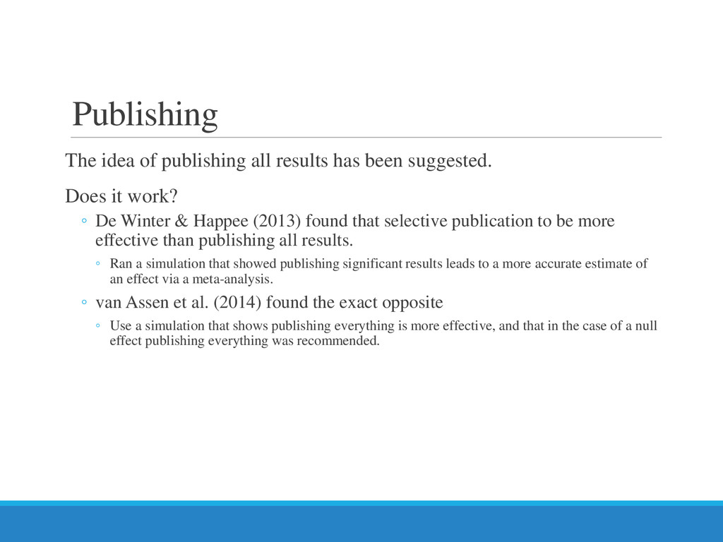
    Estimating the size of the treatment effects: Moving beyond p values. Psychiatry 6, 21-29. Moonesinghe, R., Khoury, M. J., Janssens, A. C. J. W. (2007). Most published research findings are fales- But a little replication foes a long way. PLoS Med 4 e28. Retrieved from http://www.plosmedicine.org/article/info%3Adoi%2F10.1371%2Fjournal.pmed.0040028#pmed-0040028-g002 Platt, J. R. (1964). Strong inference: Certain systematic method of scientific thinking may produce much more rapid progress than others. Science 146, 347-353. Ross, J. S., Mulvey, G. K., Hines, E. M., Nissen, S. E., Krumholz, H. M. (2009). Trial Publication after registration in clincaltrials.gov: A Cross-sectional analysis. Rossi, J. S. (1990). Statistical power of psychological research: What have we gained in 20 years? Journal of Consulting and Clinical Psychology 58, 646-656. Scragle, J. D. (2000). Publication bias: The “File-Drawer” problem in scientific inference. Journal of Scientific Exploration 14, 91- 106. Simons, D. J. (2014). The value of direct replication. Perspectives on Psychological Science 9, 76-80. Song, F., Parekh-Bhurke, S., Hooper, L., Loke, Y. K., Ryder, J. J., Sutton, A. J., Hing, C. B., & Harvey, I. (2009) Extent of publication bias in different categories of research cohorts: A Meta-analysis of empirical studies. British Medical Journal 9, 79-93. Sullivan, G. M. & Feinn, R. .(2012). Using effect size- or why P value is not enough. Journal of Graduate Medical Education 4, 279- 282. van Assen, M. A. L. M., van Aert, R. C. M., Nuijten, M. B., & Wicherts, J. M. (2014). Why publishing everything is more important then selective publishing of statistically significant results. PLoS ONE: 9, 10.1371.