Upgrade to Pro — share decks privately, control downloads, hide ads and more …

Outliers & Missing Data

Dr.Pohlig
October 24, 2014

Outliers & Missing Data

A brief, non-technical discussion of outliers & missing data for applied researchers.

Dr.Pohlig

October 24, 2014
Tweet

More Decks by Dr.Pohlig

Other Decks in Research

Transcript

  1. What is an Outlier? • An score or point that

    is far outside the range of the rest of the distribution • Two common ‘objective’ definitions • Cases that occur near or farther than three standard deviations, called a Fringelier (Wainer, 1976) • The most common definition in Introductory to Statistics textbooks were cases that are equal to or greater than 1.5 x inter-quartile range (Hogan & Evalenko, 2006) • The ‘kind’ of outlier should also be considered • Leverage measures degree a variable could be an outlier • Discrepancy measures extent to which a case is in line with others • Influence is a product of both leverage and discrepancy
  2. Causes What could cause an outlier? 1. Equipment failure or

    malfunction ◦ Instrument or Measurement error ◦ Faulty data due to human errors 2. An unlikely event drawn from a random distribution ◦ No matter how extreme an event is, it still has some probability of occurring 3. Sampled from a population that was not intended ◦ Unlikely or extreme events are rare in the real world and are not really of interest ◦ Could be multiple sub-populations have accidentally been sampled ◦ A distribution contaminating the one you are trying to examine
  3. Impact What might happen by not addressing the fact an

    outlier might exist in your data? • Can inflate within-group or error variance • Violate assumpions of the homogeneity of variance or homoscedasticity (Wilcox, 2005) • Outliers can cause the loss of power, because the samples end up coming from a contaminated normal distribution (Wilcox & Keselman, 2003) • Including outliers can bias results by creating an artificial relationship where one does not exist, or diminishing one that might truly exist.
  4. Identifying Outliers Univariately- outlier detection is fairly simple • Visual

    inspection of the data can be used • Histogram • Histograms and other methods of examining frequency distributions
  5. Identifying Outliers Box Plots • Outside value is outside the

    inner fence and denoted as o • Far-out value is outside the outer fence and denoted as * • Inner fences (IF) • Lower IF = Q1 – step • Upper IF =Q3 + step • Outer fences (OF): • Lower OF =Q1 – 2*step • Upper OF =Q3 + 2*step • Step = 1.5*IQR • IQR (Interquartile Range) = Q3-Q1
  6. Identifying Outliers Detrended Q-Q plot ◦ Quantile-Quantile plot ◦ Plots

    the observations against what would be expected to be observed if the distribution was normal ◦ Since this is detrended, a “ normal” distribution would have units cluster around the horizontal bar ◦ When looking for outliers using one- typically look to the points at most extreme and a rule of thumb is beyond ±1 may be an outlier
  7. More than one variable • Of-course in real life, we

    often have more complex phenomena we want to investigate, which involves the relationship among a number of variables • This means we have to expand our thinking to account for this expanded dimensionality. • The more variables there are, the more ways an individual data point could be an outlier • Could have an outlier, that is not an outlier on any individual variable • The intersection where the variables meet is not consistent with the rest of the observed scores • It is far away from the joint distribution of the variables • Can be hard (or may be impossible) to visualize • Even though we may not be able to visually see it, you can get the distance of any point from the rest of the data by using some measure of distance
  8. Distance • Most common is Mahalanobis’ Distance • These are

    χ2 distributed and thus can have a probability associated with them and can use a more objective strategy for removing extreme cases • Given a vector of observations = 1 , ⋯ , ′ that come from a sample having corresponding mean vector = 1 , ⋯ , ′, and covariance matrix S. • Mahalanobis’ Distance for a point is defined by = − ′− − • ′ is the transpose and − is the inverse
  9. Hidden Outliers- finding influential cases • Can calculate DFBeta’s, which

    use a Jackknife procedure, measures influence a case has on the slope estimate • Data is analyzed n+1 times. You find your estimate, � , with all of the cases included and then once with each case removed, � . • The DFBeta is then the difference between the estimate for the entire sample and when that case is removed, � − � for each i. • Then you can examine the distribution of the DFBetas for outliers. • Studentized Deleted Residuals (another Jackknife procedure) • The model is run excluding each case individually. Using the resulting model a predicated value can be found and then the residual is calculated for that case. • This residual is then “studentized”, which simply divides that value by its standard error • Other options include finding: • Leverage values- distance value from the predictors, i.e. how much a point is an outlier among predictors • Cook’s Distance (jackknife)- combines information from deleted residuals and Leverage, measures influence of one case on other cases • DFFits- change in predicted value with that case included and removed (similar to Cook’s) but now it measures influence of a case on its own predicted value
  10. Dealing with Outliers Typically, the best way of dealing with

    an outlier is simply removing it. • Should always report when data is removed • Can perform a ‘sensitivity’ analysis- run the model with and without the outlier and see what impact including it has • In small samples you can lose lots of power by removing a case • This is can lead to lots of problems when you are using procedures that require “listwise deletion” Could adjust for them or find a method that is not overly-influenced by outliers • Think of the 3 common measures of central tendency • Mean, Median, Mode- which would be robust to outliers? • What are the mean & median of the following distribution: 1,2,3,4,5 • Mean & Median = 3 • What is the mean & median of this distribution: 1,2,3,4,20? • Mean is now 6, Median is still 3
  11. Simple Solutions • Transform data • These do not specifically

    address the presence of extreme cases • The three most common transformations have been suggested (square root, logarithmic, and inverse) and occasionally outliers are remedied this way but typically this wont fix the issue, and in some instances can exaggerate it (Wilcox & Keselman, 2003) • Modifying the data points themselves to remove outliers’ influence • This is justified by saying that there is a lack of accuracy in measuring data that extreme, or data that is that extreme is not relevant (Tabachnick & Fidell, 2007) • Trimmed means, where only a certain portion of the sample is included in the analysis; [middle 80% or 85%] but still account for those cases in inferential tests (degrees of freedom are not reduced) • Winsorizing, changing the most extreme scores or outliers to the most extreme value that is considered relevant • No known standards for either procedure • Nonparametric Tests • Typically use ranked data- lose information & could lose power
  12. Robust Solutions • Robust methods to handle undue influence of

    outliers, (Chen, 2002) • All these methods work by minimizing a function that is different than what OLS minimizes • Huber has suggested the use of a robust method (robust against outliers and extreme data points) by finding a weight for each score, and then multiplying the score by the weight (Fox, 2002) • These methods minimize a function of Weighted Least Squares (WLS) • This can help reduce outliers’ effects by weighting cases in relation to its distance from the median, since outliers influence the mean • The further from the median the less weight the case could be given • Huber also developed robust methods for maximum likelihood estimation (Huber, 1972) • Maximum likelihood estimation, first proposed by Fisher, is a statistical method used to maximize the likelihood of estimating the population parameters from the underlying probability distribution from the data sampled (Tabachnick & Fidell, 2007; Aldrich, 1997). • Iteratively reweighted least squares (IRLS) computes the weighting and then reweights by using the procedure iteratively
  13. Robust cont. • Most common method is Huber’s IRLS based

    on the Median Absolute Deviation (MAD) • The MAD is calculated by finding the median, subtracting all the scores from the median, giving a deviation or error value (ei ), and then finding the median value of these errors • This is multiplied by the constant, 1/.6745 • Using the MAD value, you can then find the weight to apply to each case, as well as determine which cases should be weighted. • This is applied iteratively till weights become stable (fail to change/converge)             − × = ∧ ∧ i i median Median MAD ε ε 6745 . 1 u i = e i MAD w i = 1 u i =1.345 1.345 u i u i >1.345       
  14. Missing Data • Is missing data a problem? • How

    can data be missing? (Not what could cause data to be missing)
  15. Missingness • Sometimes missing data is planned for or expected

    • Imagine creating an achievement test, initially you will have too many items to give to each individual • Can randomly give items to individuals and then link them later using items that people have in common • An event happening signifies the last measurement (Survival Analysis) • Is missing data a problem? • Most analyses are not design to handle missing data • The degree to which it may be problematic depends on two factors 1. Amount of Missing 2. Type of Missing ◦ The type of missing data is more often a bigger problem than the actual amount of missing • More variables you have, the greater the pattern of missing you can have • For each n variables the potential number of missing patterns is 2n • Generally missing data can be classified into 3 categories (Little & Rubin, 1987)
  16. MCAR Missing Completely at Random (MCAR) | , 𝑢𝑢𝑢𝑢𝑢𝑢𝑢𝑢 =

    | • The data missing is independent of [not related to] both unobserved (missing) and observed values of other variables • The distribution of outcomes in observed individuals is a representative sample of the distribution of outcomes in the overall population • A special case is Covariate Dependent Missing Completely at Random (CD-MCAR) • This can be found in studies with repeated measurements (within-subjects designs) • Missing data may depend on observed baseline covariates but is independent of the successive missing and observed outcomes
  17. MAR Missing at Random (MAR) | , 𝑢𝑢𝑢𝑢𝑢𝑢𝑢𝑢 = |

    • The data missing is independent of unobserved (missing) values of other variables • The probability that data is missing is independent of unobserved values, given the observed data in the data set • Any systematic difference between the observed and unobserved values can be explained by differences in the data that was observed/measured & not missing (present) • For example, maybe individuals with very low scores on an observed covariate may be more likely to have missing data on a certain outcome
  18. MNAR Missing Not at Random (MNAR) • There is no

    simplified equation to explain this • Also called non-ignorable missing • The data missing is dependent on both the unobserved (missing) values and observed values of other variables • Given all the observed data, the probability that data are missing is also dependent on unobserved values • For example, maybe individuals with worse outcomes may be more likely to have missing data on outcomes
  19. WTF am I talking about? • How can something be

    missing at random, but not be missing completely at random? How can something be missing but dependent upon observed but not unobserved variables? • MCAR • For example this is what you would typically think of as ‘randomly’ missing • MAR • People who score very high on the SATs rarely have a second SAT score • MNAR • People who have no intention of going to college will rarely have an SAT score
  20. Visually Complete MCAR MAR MNAR 0 53 0 53 0

    53 0 53 2 61 2 61 2 61 2 61 6 70 6 - 6 70 6 70 7 47 7 47 7 47 7 47 8 38 8 38 8 38 8 38 9 53 9 - 9 53 9 53 11 47 11 - 11 - - - 14 53 14 53 14 - - - 15 43 15 - 15 - - - 18 37 18 37 18 - - -
  21. Visually Complete MCAR MAR MNAR 0 53 0 53 0

    53 0 53 2 61 2 61 2 61 2 61 6 70 6 - 6 70 6 70 7 47 7 47 7 47 7 47 8 38 8 38 8 38 8 38 9 53 9 - 9 53 9 53 11 47 11 - 11 - - - 14 53 14 53 14 - - - 15 43 15 - 15 - - - 18 37 18 37 18 - - -
  22. Visually Complete MCAR MAR MNAR 0 53 0 53 0

    53 0 53 2 61 2 61 2 61 2 61 6 70 6 - 6 70 6 70 7 47 7 47 7 47 7 47 8 38 8 38 8 38 8 38 9 53 9 - 9 53 9 53 11 47 11 - 11 - - - 14 53 14 53 14 - - - 15 43 15 - 15 - - - 18 37 18 37 18 - - -
  23. Visually Complete MCAR MAR MNAR 0 53 0 53 0

    53 0 53 2 61 2 61 2 61 2 61 6 70 6 - 6 70 6 70 7 47 7 47 7 47 7 47 8 38 8 38 8 38 8 38 9 53 9 - 9 53 9 53 11 47 11 - 11 - - - 14 53 14 53 14 - - - 15 43 15 - 15 - - - 18 37 18 37 18 - - -
  24. Visually Complete MCAR MAR MNAR 0 53 0 53 0

    53 0 53 2 61 2 61 2 61 2 61 6 70 6 - 6 70 6 70 7 47 7 47 7 47 7 47 8 38 8 38 8 38 8 38 9 53 9 - 9 53 9 53 11 47 11 - 11 - - - 14 53 14 53 14 - - - 15 43 15 - 15 - - - 18 37 18 37 18 - - -
  25. Testing Missingness • Little (1988) created a test based on

    Maximum Likelihood enabling researchers to test if data is MCAR • Can use this test to see if means are different between cases with missing and non-missing data • If MCAR is true, there will be no difference between means • Further generalized it to test if the Covariance Matrices are different between cases with and without data • If MCAR is true, there will be no difference between Covariance Matrices • Kim & Bentler (2002) created a test based on Generalized Least Squares (GLS) • Can test Means, Covariance Matrices, and both of those simultaneously • As of now, no independent test of MNAR (the important one), can pseudo test this using statistical models • These tests have plenty of limitations (i.e. data have to meet normality,…)
  26. What Can you do? • Listwise deletion- only include cases

    with complete data • Lose power • Assumes MCAR • Pairwise deletion- include cases when data is available • Leads to funky n’s • Assumes MCAR • Can lead to non-positive definite matrices, eliminates the restriction of range that is logically needed • If you know r12 and r23 , r13 can only be in a certain range • Inverse Probability Weighting (IPW) • Model the probability of an observation being observed or not, and then weight cases by 1/probability of being observed
  27. Impute values • Mean imputation- insert the mean of a

    variable for every instance of missing • Biases estimates of every statistic/parameter but the mean • Greatly reduces variability • Does this no matter the type of missing (MCAR, MAR, or MNAR) • Regression imputation- use a regression equation to insert the predicted value given all the observed data for a case • Biases the covariance between variables by inflating it • Linearizes data as formerly missing data now fall on the regression line • Data must be MAR or MCAR • Last Values Carried Forward- (LVCF) for repeated measure designs • Typically considered for clinical trials to deal with drop out • Simply use the last values observed, and impute them for the rest of observations • Will typically lead to a conservative estimate as most often we expect differences to become greater over time given some treatment
  28. More advanced • Expectation-Maximization algorithm (Dempster, Laird, & Rubin, 1977)

    • Conceptually this is like using a model (regression imputation) and then adding random error to cases then analyze with model of interest- different variables can be in the two models • Obtains M-L estimators in incomplete data using IRLS • Assumes multivariate normality (but is robust to moderate violations) • Data must be MAR or MCAR • Can only impute continuous (interval or ratio) data • Linerizes data, but to a much smaller extent than regression imputation • Multiple imputation procedure (Rubin, 1987) • Creates multiple data sets, with different values imputed (typically uses E-M) • The estimates are than averaged across the data sets • Data must be MAR or MCAR • Performance is limited by the amount of missing data (for very low missing it works well) • Does this by generating random samples from a posterior probability distribution need to choose a Bayesian method (i.e. Markov Chain Monte Carlo, etc.) • If imputing a sensitivity analysis should be performed showing how the imputation changed the estimates
  29. Maximum Likelihood • ML is an alternative to OLS and

    can be adapted and used in more sophisticated analyses • Creates a Likelihood Function that gets maximized vs simply minimizing sum of squared errors • The Likelihood is the multiplication of the joint probability distribution across all individuals for all variables and parameter estimates • Observed variable values are known, therefore we find the values for the parameters that maximize the likelihood function (iterative process) • We are interested in finding the marginal probabilities, therefore we can integrate across the missing data • By integrating over the variables with missing data, we can get the probability of observing variables that have actually been observed • Conceptually, we are only looking at data when it is present • This is a “Full-Information” method • Data must be MAR or MCAR
  30. ML • For n observations = 1, … , on

    k variables, 𝒌 = 𝑖 , … , • With no missing data Likelihood function is = � =1 𝒌; • With � is the joint probability function for observation i, and is the set (vector) of parameters to be estimated. • To get ML estimates, simply find values of that maximize because 𝒌 is observed • If variables for an individual case are missing, the � can be found without using those variables using a new function, ∗ � • This is done integrating out missing values, which enables us to calculate the marginal probabilities as if they had data present. • This would change the to be a multiplicitave of all the ∗ � ’s and � .
  31. ML part 2 • For instance if in a sample

    individuals’ data are missing for the first variable • Given here in scalar form ∗ 2 , … , 𝑖𝑖 ; = � 1 𝑖 , … , 𝑖𝑖 1 • Then the likelihood function is defined as the product of the function for individuals with all the data multiplied by the function for individuals with missing the data on y1 , ∗ = � =1 𝑖 , … , 𝑖𝑖 ; × � +1 ∗ 2 , … , 𝑖𝑖 ; • Where an m observations have complete data and n-m have data missing. • If the missing data are discrete, the joint probability is found by summing the probabilities across all values that could be taken • †Equations adapted from Allison (2012)
  32. Solutions • Most often small amounts of missingness can be

    ignored or ‘fixed’ by using listwise/pairwise deletion. • The catch-22: • MI & ML are “large sample” methods, and are generally recommended for research including lots of individuals (not necessarily observations) • Because methods are iterative having small samples can lead to convergence failures • If you have a large n, ignoring the missingness using deletion is probably OK • Personally, I lean towards ML over MI (Allison, 2012) • ML is technically more asymptotically efficient (minimize sample variance), MI would be efficient if you could produces an infinite number of data sets • ML is consistent- not matter how many times you run the analysis you will always reach same conclusion, this is not true in MI (the idea of MI is to average across replications that introduce error) • ML does not require a choice (in MI- need to choose Bayesian method, prior, number of times, etc.) • MI requires you to specify an imputation model & analysis model which could be in contrast to each other • What if MNAR?
  33. Heckman If MNAR by definition the missing is a function

    of both observed and unobserved variables, and thus you would have to model this. • Heckman Regression- was created to handle selection bias but can be used with MNAR • Strongly assumes multivariate normality, model is unidentifiable if this is not met • This method was designed for situations in which the dependent variable in a linear regression model is missing for some cases but not for others • A two-step approach • First step is to build a model that predicts if you have data missing or not using a Probit model • Typically use all the predictors you can, regardless of whether they are going to predict the outcome of interest • Use residuals generated to create a new variable • Second step is to build the model of interest and include the new variable from the first step as a predictor • This second step tests for bias if the new variable is significant, you have found selection bias • Also adjust for the bias by including the variable
  34. Goal of Science • What is often the main goal

    of a line of research? Not the proximal but the ultimate goal • Showing Causality or in a weaker sense of that word, the effect of one variable on another • To show Causality three conditions are needed: 1) Correlation- there must be a relationship 2) Proper time order must be established 3) No confounding or extraneous variables explain the phenomena/elimination of rival hypotheses • Why is causality so hard to get at? • Almost impossible to account for all Internal Validity threats • Counterfactual Inference • Counterfactual question is: What would have happened to that person if they had a different value on the IV. • What would outcome have been for those who received a treatment, if they had not received treatment (or vice-versa)? • Counterfactuals cannot be observed
  35. Effect • For brevity, I will talk about a Treatment

    Effect, , on one outcome • Being in one specific condition and getting a treatment that is distinctly different than what other conditions receiving • How could we operationally define a , such that it could be measured? • Causal effect for a given subject is measured by examining the difference in an outcome/dependent variable (DV) with and without treatment, = 1 − 0 • 1 is the subject’s outcome with the treatment; 0 without treatment • The average treatment effect is then the expected value of that difference across the population = 1 − 0 • � is the expectation operator
  36. Causality • It is not possible to observe an individual’s

    unbiased treatment effect • We do not know the outcome for untreated observations getting the treatment, and for treated when they do not get treatment • What is the standard way of showing causality? • “True Experiments” or Randomized Controlled Trials (RCT) are the ‘gold standard’ • How do these work? • Participants randomly assigned to treatment conditions • Randomization must be true • What does randomization accomplish? • Eliminating potential bias in treatment assignment • It removes the need to worry about covariates/confounders/potential rival hypotheses • Achieves balance- all covariates (observed & unobserved) should be equally distributed among the conditions
  37. Causal Evidence • If you can’t randomly assign people, you

    introduced selection and/or allocation bias • This means the internal validity of your study is reduced • Any difference in outcomes could be due to this selection/allocation bias and not the treatment • If we have measured/observed the variables that are contributing to the bias as we can just include them as covariate in the analysis and adjust for the differences, but this doesn’t always work and can cause other problems in model estimation (lose power, complicate analyses, etc.) • Why are am I talking about this? • Rubin in late 70’s-80’s reframed idea of not being able to observe the counterfactual as a missing data problem • Treating the unobservable counterfactual as a missing data problem means that methods for resolving selection bias can be used to garner causality from non-experimental/non-RTC designs Group 1 0 Treatment (D = 1) Observable Counterfactual Control (D=0) Counterfactual Observable Group 1 0 Treatment (D = 1) Observed Missing Control (D=0) Missing Observed
  38. Causality via Non-RCTs • While counterfactuals cannot be observed, they

    can be estimated • Propensity scores (PS) can be used for this • A Propensity score is the probability of getting a treatment given a vector of observed variables, = 1| , where is the observed predictors. • PS can be used for matching or as covariates, alone or with other matching variables and covariates. • Similar to the Heckman Regression propensity score methods are two-staged ◦ The predicted probability of receiving the treatment is obtained from logistic regression, which allows us to create a counterfactual group ◦ When a member of the treatment group is matched to a member of the control group using the propensity score, both are considered to have the same probability of being in the treatment condition but one got the treatment and the other did not ◦ In the next step, the PS are used in the model that is testing the relationship of interest ◦ After matching the treatment with control group units, the treatment effect can then be analyzed by comparing outcome variable(s) for the two groups
  39. Propensity Scores • Propensity scores should balance the data, as

    those with similar probabilities of getting treatment, probably have similar values on the measured variables • You can test this using t-tests, and χ2 tests • Common Support is imposed by dropping treatment subjects whose propensity scores is higher than the maximum or less than the minimum propensity score of the controls • You cannot compare groups who have no match in the other group (can get around this by using PS Stratification or Weighting) • Number of different ways to match individuals or could weight by inverse of PS • Requires large sample sizes to ensure good matching, typically large numbers of covariates are collected to make sure match is best • Does not address unobserved covariates
  40. Outlier References Aldrich, J. (1997). R. A. Fisher and the

    making of maximum likelihood 1912 – 1922. Statistical Science, 12, 162-176 Chen, Colin (2002). Robust Regression and Outlier Detection with the ROBUSTREG procedure. SUGI Paper 265-27. SAS Institute: Cary, NC. Fox, J. (2002). An R and S-PLUS companion to applied regression. Thousand Oaks, CA: Sage Publications, Appendix robust regression 1-8. Hogan, T. P. & Evalenko K. (2006). The elusive definition of outliers in introductory statistics textbooks for behavioral sciences. Teaching of Psychology, 33, 247-275. Huber, P. J. (1964). Robust estimation of a location parameter. The Annals of Mathematical Statistics, 35, 73-101. Tabachnick, B. G., & Fidell, L. S. (2007). Using Multivariate Statistics (5th ed). Boston, MA: Allyn and Bacon, 77. Wainer, H. (1976). Robust statistics: A survey and some prescriptions. Journal of Educational Statistics, 1(4), 285-312. Wilcox, R. R. (2005). New methods for comparing groups: Strategies for increasing the probability of detecting true differences. Current Directions in Psychological Science, 14, 272- 275. Wilcox, R. R. & Keselman, H. J. (2003). Modern robust data analysis methods: Measures of central tendency. Psychological Methods, 8, 254-274.
  41. Missing Data References Allison, P. D. (2012). Handling Missing Data

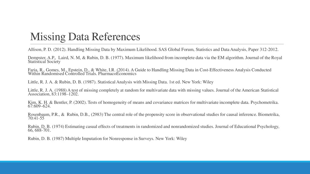
    by Maximum Likelihood. SAS Global Forum, Statistics and Data Analysis, Paper 312-2012. Dempster, A.P., Laird, N. M, & Rubin, D. B. (1977). Maximum likelihood from incomplete data via the EM algorithm. Journal of the Royal Statistical Society Faria, R., Gomes, M., Epstein, D., & White, I.R. (2014). A Guide to Handling Missing Data in Cost-Effectiveness Analysis Conducted Within Randomised Controlled Trials. PharmacoEconomics Little, R. J. A. & Rubin, D. B. (1987). Statistical Analysis with Missing Data. 1st ed. New York: Wiley Little, R. J. A. (1988) A test of missing completely at random for multivariate data with missing values. Journal of the American Statistical Association, 83:1198–1202. Kim, K. H. & Bentler, P. (2002). Tests of homogeneity of means and covariance matrices for multivariate incomplete data. Psychometrika. 67:609–624. Rosenbaum, P.R., & Rubin, D.B., (2983) The central role of the propensity score in observational studies for causal inference. Biometrika, 70:41-55 Rubin, D. B. (1974) Estimating casual effects of treatments in randomized and nonrandomized studies. Journal of Educational Psychology, 66, 688-701. Rubin, D. B. (1987) Multiple Imputation for Nonresponse in Surveys. New York: Wiley