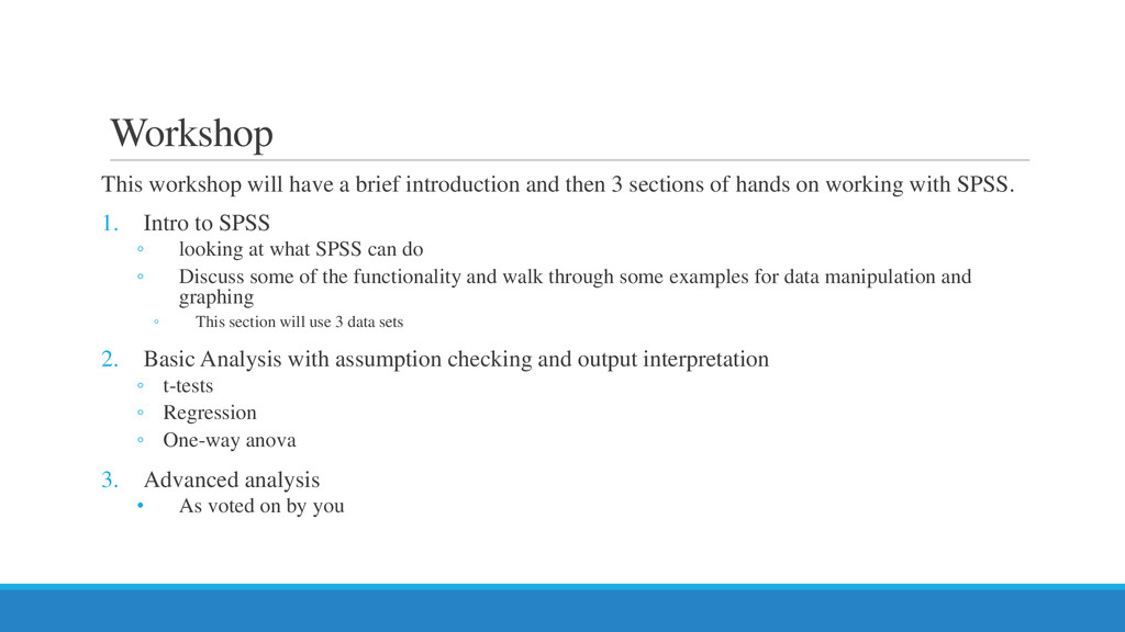
3 sections of hands on working with SPSS. 1. Intro to SPSS ◦ looking at what SPSS can do ◦ Discuss some of the functionality and walk through some examples for data manipulation and graphing ◦ This section will use 3 data sets 2. Basic Analysis with assumption checking and output interpretation ◦ t-tests ◦ Regression ◦ One-way anova 3. Advanced analysis • As voted on by you
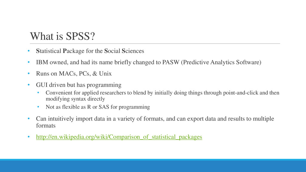
• IBM owned, and had its name briefly changed to PASW (Predictive Analytics Software) • Runs on MACs, PCs, & Unix • GUI driven but has programming • Convenient for applied researchers to blend by initially doing things through point-and-click and then modifying syntax directly • Not as flexible as R or SAS for programming • Can intuitively import data in a variety of formats, and can export data and results to multiple formats • http://en.wikipedia.org/wiki/Comparison_of_statistical_packages
IDRE (Institute for Digital Research and Education): http://www.ats.ucla.edu/stat/spss/ ◦ The IDRE is the best site I’ve seen for stats software help & guides Add-Ons ◦ SPSS has a number of add-ons that you can purchase ◦ AMOS- SEM software ◦ Big Data tools ◦ Statistics Server- lets you work using data off your server ◦ Modeler- data mining tool ◦ Data collection- create surveys that can be deployed on web or mobile devices ◦ Sample Power- power analysis ◦ Text Analytics- used for text and open ended items/variables
Dataset • Data View – spreadsheet containing actual data • Variable View – contains the information about the variables • Syntax – lets you edit the commands directly using syntax (SPSS’ ‘code’) • Output – Displays the output from procedures run, and errors when encountered • If you are unsure use the help feature! It is surprisingly helpful
the having actual data • Let’s create some fake data, one continuous (Score) and one dichotomous variable (Sex) • Menus • Data & Transform • Used for Manipulating Data • Analyze • Used to get statistics & results • Graphs • Used for getting some visual output • Toolbar
Excel • Does not have functions like excel • Variables are Columns • Rows are cases • Can cut, paste, reorder both variables and cases • SPSS has no row or column limit • For those using 32 bit the theoretical limit on rows and columns spss can handle is • (2^32)-1 > 2 billion • Leave missing data blank, it is just easier that way!
letter • Cannot contain a space (use underscore _) • I would advise NOT ending a variable with an underscore as some variables created through procedures in SPSS do this also and may overwrite what you had • Cannot end with a period • Variable names must be unique Type • String & Numeric are most frequent • Variety of Date & Currency formats • Choosing String when it is a Numeric variable will eliminate the way the variable can be used in some analyses Measure • Use Nominal for string variables • Scale for everything else
can put in free form text to describe exactly what the variable is • Caution: this will show up in the output so stay away from very long descriptions or unhelpful ones (these do not have to be unique) Missing • If you did use a specific value for missing you can indicate that here Values • When variables have multiple levels that have specific meanings, you put that information here so that it shows up in the output • For example • Males coded as 0, Females coded as 1 • A 1 stands for strongly disagree, 2 disagree, 3 neutral, 4 agree, 5 strongly agree
• Click on “File Type” drop down menu • Choose excel files • Select the “Homework” data file called (HW_data) • Can choose which worksheet in excel the data comes from • Make sure to check that variable names are first row • Lets try a CSV file • Choose either all or Text in drop down • Import wizard comes up to help you Exporting Data • Go to Save As • Select the format you want to save the file as in the drop down menu • Variables button lets you choose if you want to save the entire file or remove some variables
is used to create new variables • Can be entirely novel • Can be a function of other variables already present • Has a lot of options, like using functions in excel • Has a way to incorporate an if statement for conditional logic • Creating a difference score • Name the new variable, move over posttest, click ‘-’ move over pretest • Hit Paste, which will send the commands to the syntax window Useful Compute commands • Algebraic manipulations: ln, SQRT • $Casenum – creates a value for each case that indicates its row number (easy way to make an ID variable) • Datediff – lets you find the differences in dates. • Any – lets you search for a value or character in a variable • Create a mean test score • Name new variable testaverage • Find the Mean function and click the up arrow • Select pretest and posttest to insert in parentheses
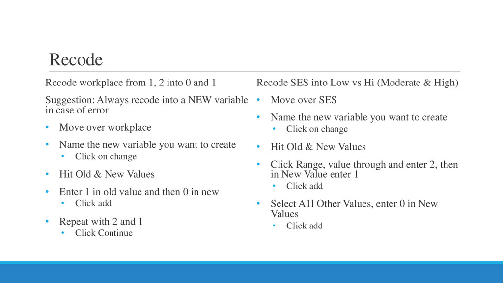
Suggestion: Always recode into a NEW variable in case of error • Move over workplace • Name the new variable you want to create • Click on change • Hit Old & New Values • Enter 1 in old value and then 0 in new • Click add • Repeat with 2 and 1 • Click Continue Recode SES into Low vs Hi (Moderate & High) • Move over SES • Name the new variable you want to create • Click on change • Hit Old & New Values • Click Range, value through and enter 2, then in New Value enter 1 • Click add • Select A1l Other Values, enter 0 in New Values • Click add
by numerical or alphabetical value • Split file • Compare Groups or Organize Output by Groups • This command lets you run any procedure for each group separately • If used for analysis no between comparisons will be printed Select Cases • This is used to filter out data when doing analyses • Can specify an if statement • Use an already created filter variable
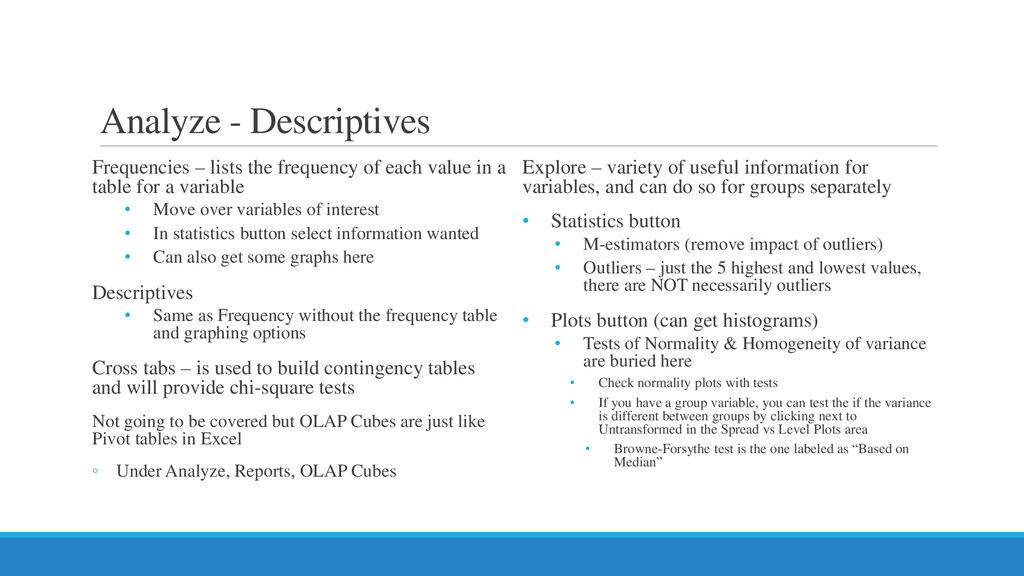
value in a table for a variable • Move over variables of interest • In statistics button select information wanted • Can also get some graphs here Descriptives • Same as Frequency without the frequency table and graphing options Cross tabs – is used to build contingency tables and will provide chi-square tests Not going to be covered but OLAP Cubes are just like Pivot tables in Excel ◦ Under Analyze, Reports, OLAP Cubes Explore – variety of useful information for variables, and can do so for groups separately • Statistics button • M-estimators (remove impact of outliers) • Outliers – just the 5 highest and lowest values, there are NOT necessarily outliers • Plots button (can get histograms) • Tests of Normality & Homogeneity of variance are buried here • Check normality plots with tests • If you have a group variable, you can test the if the variance is different between groups by clicking next to Untransformed in the Spread vs Level Plots area • Browne-Forsythe test is the one labeled as “Based on Median”
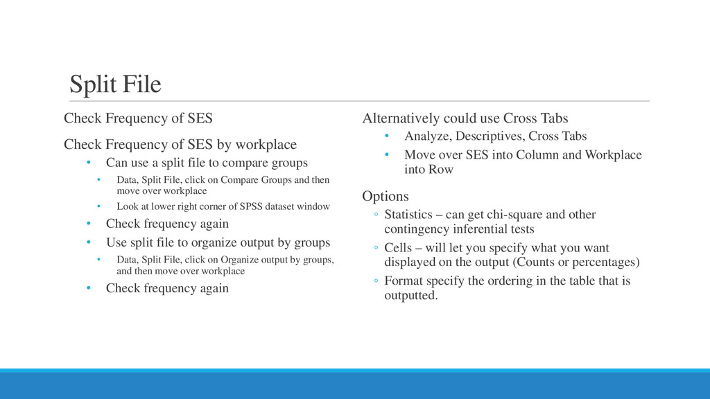
by workplace • Can use a split file to compare groups • Data, Split File, click on Compare Groups and then move over workplace • Look at lower right corner of SPSS dataset window • Check frequency again • Use split file to organize output by groups • Data, Split File, click on Organize output by groups, and then move over workplace • Check frequency again Alternatively could use Cross Tabs • Analyze, Descriptives, Cross Tabs • Move over SES into Column and Workplace into Row Options ◦ Statistics – can get chi-square and other contingency inferential tests ◦ Cells – will let you specify what you want displayed on the output (Counts or percentages) ◦ Format specify the ordering in the table that is outputted.
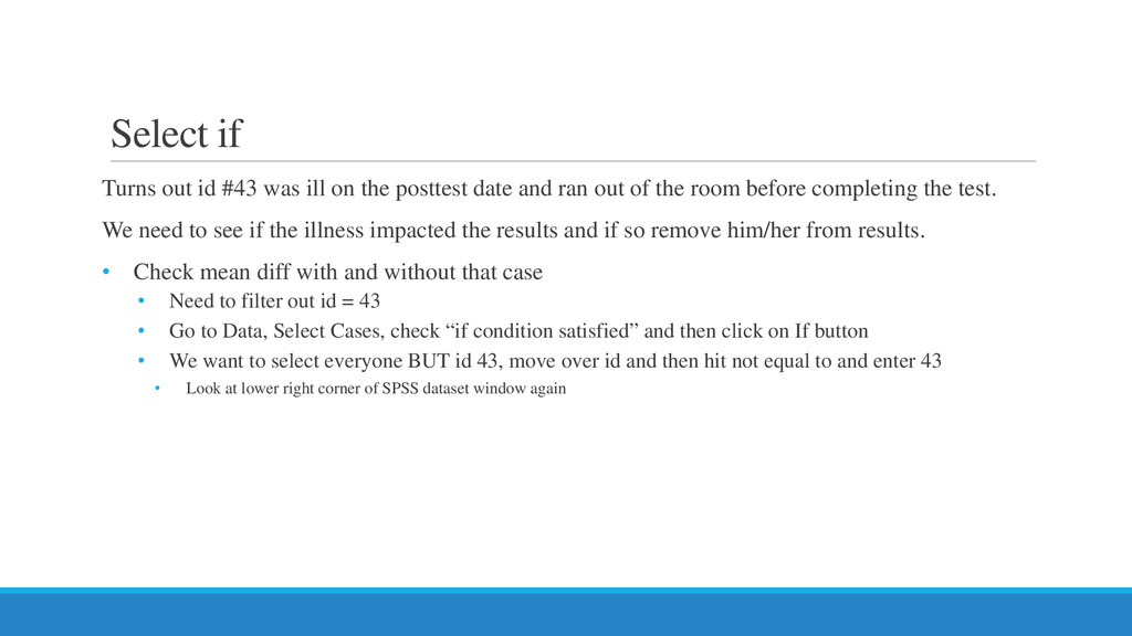
posttest date and ran out of the room before completing the test. We need to see if the illness impacted the results and if so remove him/her from results. • Check mean diff with and without that case • Need to filter out id = 43 • Go to Data, Select Cases, check “if condition satisfied” and then click on If button • We want to select everyone BUT id 43, move over id and then hit not equal to and enter 43 • Look at lower right corner of SPSS dataset window again
“followup” but this is contained in a different excel file called “HW_data_addendum” We want to add the follow up scores • Old School method, can copy and paste the values into the data viewer • Can merge data sets • First save the HM_data as an spss file (.sav extension) • Open up the addendum in SPSS, and save that as an spss file • Make sure the “key” variable that you will be matching on is sorted ascending • Go to Data, Merge Files • Add variables, and navigate the location of the saved addendum file • SPSS is ‘smart’ enough to know what is unique • Click Match cases on Key variable (and that it is sorted) • Select id and move it into the key variables box
test scores, each as its own variable • This is the “wide” format of data • What if we wanted to switch to the “long” format for the data? • Where each measurement occasion is a unique case? • Use the “restructure” wizard, in the data menu • What do we want to do? We want to take variables and turn them into cases (first choice) • Hit next • Since we are only transposing the 1 variable, we choose top option • Hit next ◦ Leave the identifier as id ◦ In the variables to be transposed, we want to name the variable that will be made out of the three test scores, call it score ◦ Move over the three test scores ◦ All the other variables will be fixed, ◦ Move them into fixed box ◦ We do want an index variable, which will indicate the measurement occasion based on the order we chose ◦ Index =1 will be pretestscore ◦ Index=2 will be posttestscore ◦ Index=3 will be followup ◦ You can choose to rename index if you want ◦ Hit finish
in SPSS, you have already seen some of them and some will be covered later • What does the distribution of all the scores look like? • Graphs, Legacy Dialogues, Histograms • See if score is related to time using a scatter plot • Graphs, Legacy Dialogues, Scatter/Dot, Simple Scatter, and hit define • Move over the Score variable to the Y axis, and Index (or time) to the X axis and hit Ok • Double click on the graph and add a trendline • Looks like a tend over time, but what is wrong with doing it like this? • What if you wanted to do some multi-level modeling and wanted to see if there was a trend over time of the test scores? • Do the same scatterplot as before, but now set marker by id • Double click on graph and now we can add 2 different trend lines, an individual one and an aggregated one • Click on add fitline at subgroups • Click on add fitline at total (click on lines and make the weight 3 to see it better) • Export that to an excel file by right clicking and choosing export or go to file export
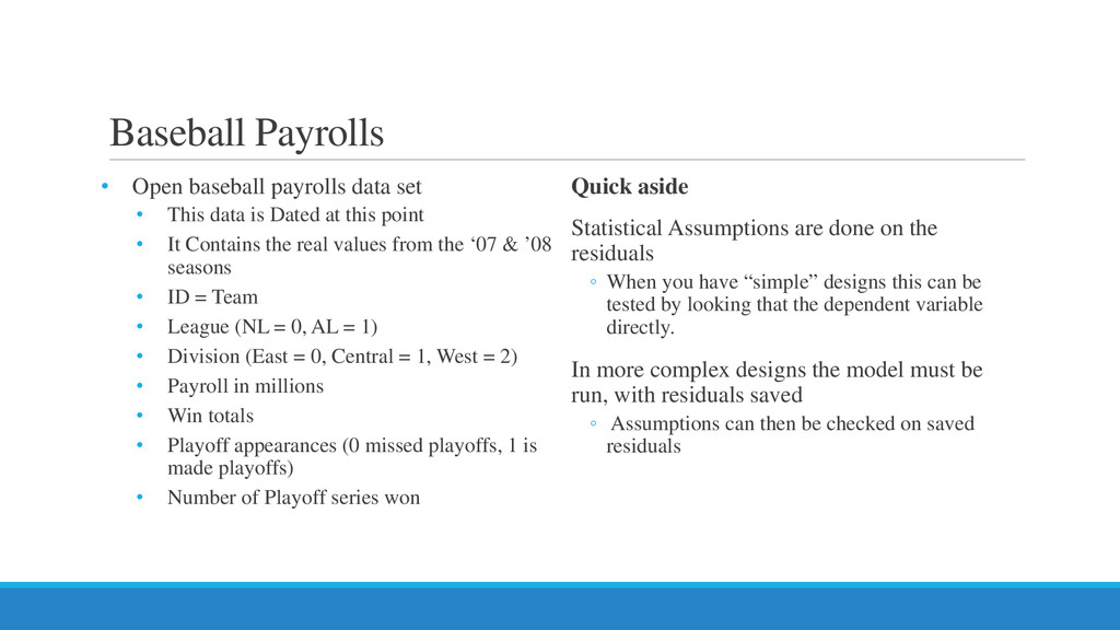
data is Dated at this point • It Contains the real values from the ‘07 & ’08 seasons • ID = Team • League (NL = 0, AL = 1) • Division (East = 0, Central = 1, West = 2) • Payroll in millions • Win totals • Playoff appearances (0 missed playoffs, 1 is made playoffs) • Number of Playoff series won Quick aside Statistical Assumptions are done on the residuals ◦ When you have “simple” designs this can be tested by looking that the dependent variable directly. In more complex designs the model must be run, with residuals saved ◦ Assumptions can then be checked on saved residuals
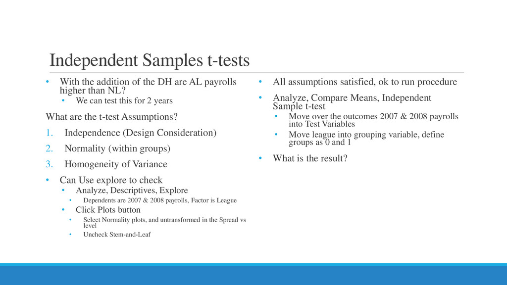
are AL payrolls higher than NL? • We can test this for 2 years What are the t-test Assumptions? 1. Independence (Design Consideration) 2. Normality (within groups) 3. Homogeneity of Variance • Can Use explore to check • Analyze, Descriptives, Explore • Dependents are 2007 & 2008 payrolls, Factor is League • Click Plots button • Select Normality plots, and untransformed in the Spread vs level • Uncheck Stem-and-Leaf • All assumptions satisfied, ok to run procedure • Analyze, Compare Means, Independent Sample t-test • Move over the outcomes 2007 & 2008 payrolls into Test Variables • Move league into grouping variable, define groups as 0 and 1 • What is the result?
increase over time? • We can test if there was a significant change between 2007 and 2008 What are the Assumptions? 1. Independence (Design Consideration) 2. Normality of difference scores Need to create difference score by using compute command ◦ Paydiff = 2008 payroll – 2007 payroll ◦ Use Explore on paydiff with no factors for normality test What is result? ◦ Ignore for a second and then we will fix it Analyze, Compare Means, paired Samples t-test ◦ Move over 2007 & 2008 payroll variables ◦ What is result? What about that assumption violation ◦ Looks negatively skewed ◦ How could this be fixed? ◦ Taking SQRT of diff ◦ The run a 1 sample t-test on difference score compared to 0 ◦ Compute paydiff_sqrt = SQRT(paydiff) Analyze, Compare Means, one Samples t-test ◦ Move over paydiff_sqrt ◦ What is result?
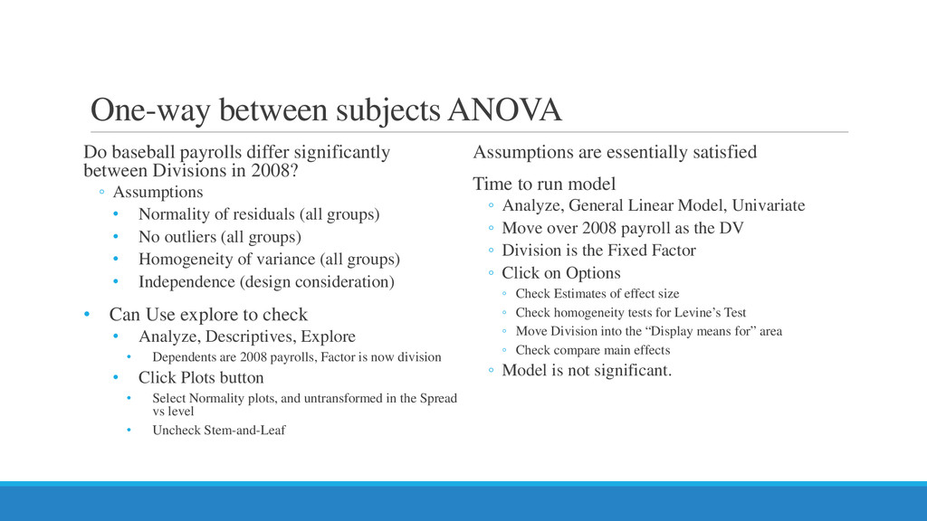
Divisions in 2008? ◦ Assumptions • Normality of residuals (all groups) • No outliers (all groups) • Homogeneity of variance (all groups) • Independence (design consideration) • Can Use explore to check • Analyze, Descriptives, Explore • Dependents are 2008 payrolls, Factor is now division • Click Plots button • Select Normality plots, and untransformed in the Spread vs level • Uncheck Stem-and-Leaf Assumptions are essentially satisfied Time to run model ◦ Analyze, General Linear Model, Univariate ◦ Move over 2008 payroll as the DV ◦ Division is the Fixed Factor ◦ Click on Options ◦ Check Estimates of effect size ◦ Check homogeneity tests for Levine’s Test ◦ Move Division into the “Display means for” area ◦ Check compare main effects ◦ Model is not significant.
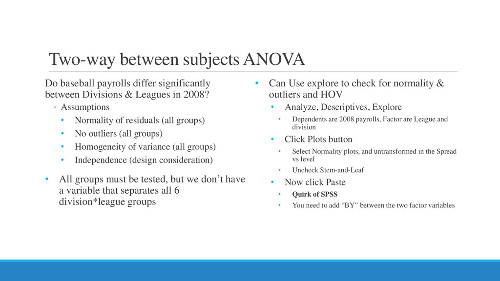
Divisions & Leagues in 2008? ◦ Assumptions • Normality of residuals (all groups) • No outliers (all groups) • Homogeneity of variance (all groups) • Independence (design consideration) • All groups must be tested, but we don’t have a variable that separates all 6 division*league groups • Can Use explore to check for normality & outliers and HOV • Analyze, Descriptives, Explore • Dependents are 2008 payrolls, Factor are League and division • Click Plots button • Select Normality plots, and untransformed in the Spread vs level • Uncheck Stem-and-Leaf • Now click Paste • Quirk of SPSS • You need to add “BY” between the two factor variables
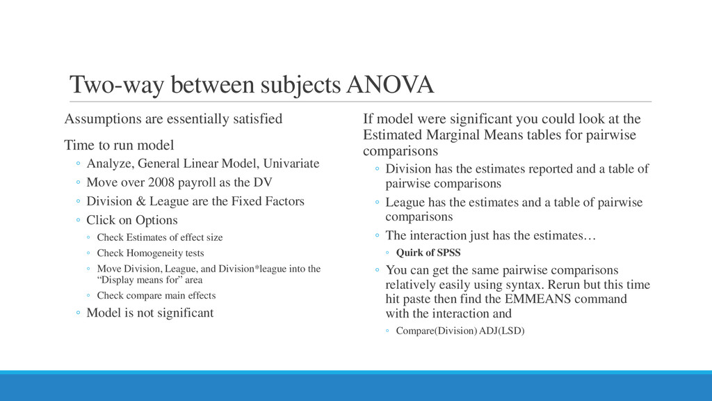
Marginal Means tables for pairwise comparisons ◦ Division has the estimates reported and a table of pairwise comparisons ◦ League has the estimates and a table of pairwise comparisons ◦ The interaction just has the estimates… ◦ Quirk of SPSS ◦ You can get the same pairwise comparisons relatively easily using syntax. Rerun but this time hit paste then find the EMMEANS command with the interaction and ◦ Compare(Division) ADJ(LSD) Assumptions are essentially satisfied Time to run model ◦ Analyze, General Linear Model, Univariate ◦ Move over 2008 payroll as the DV ◦ Division & League are the Fixed Factors ◦ Click on Options ◦ Check Estimates of effect size ◦ Check Homogeneity tests ◦ Move Division, League, and Division*league into the “Display means for” area ◦ Check compare main effects ◦ Model is not significant Two-way between subjects ANOVA
2007 and 2008? • Will talk about assumptions in next procedure for Regression • Want a correlation matrix made up for 4 variables • Analyze correlate bivariate, move over the variables of interest • Below you can check the box for Spearman’s Rank correlation if you violate some of the assumptions • What do we see? Regression • What if we want to see the impact of change in payroll on 2008 win total but we want to adjust for potential confounder of 2007 win payroll? • Need to use multiple regression, predicting 08 win total by paydiff and including 07 payroll in the model
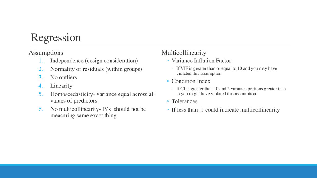
(within groups) 3. No outliers 4. Linearity 5. Homoscedasticity- variance equal across all values of predictors 6. No multicollinearity- IVs should not be measuring same exact thing Multicollinearity ◦ Variance Inflation Factor ◦ If VIF is greater than or equal to 10 and you may have violated this assumption ◦ Condition Index ◦ If CI is greater than 10 and 2 variance portions greater than .5 you might have violated this assumption ◦ Tolerances ◦ If less than .1 could indicate multicollinearity
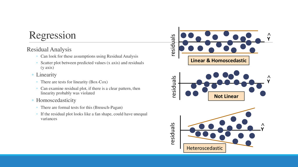
Residual Analysis ◦ Scatter plot between predicted values (x axis) and residuals (y axis) ◦ Linearity ◦ There are tests for linearity (Box-Cox) ◦ Can examine residual plot, if there is a clear pattern, then linearity probably was violated ◦ Homoscedasticity ◦ There are formal tests for this (Breusch-Pagan) ◦ If the residual plot looks like a fan shape, could have unequal variances Not Linear Linear & Homoscedastic Y residuals residuals < Heteroscedastic Y residuals < Y <
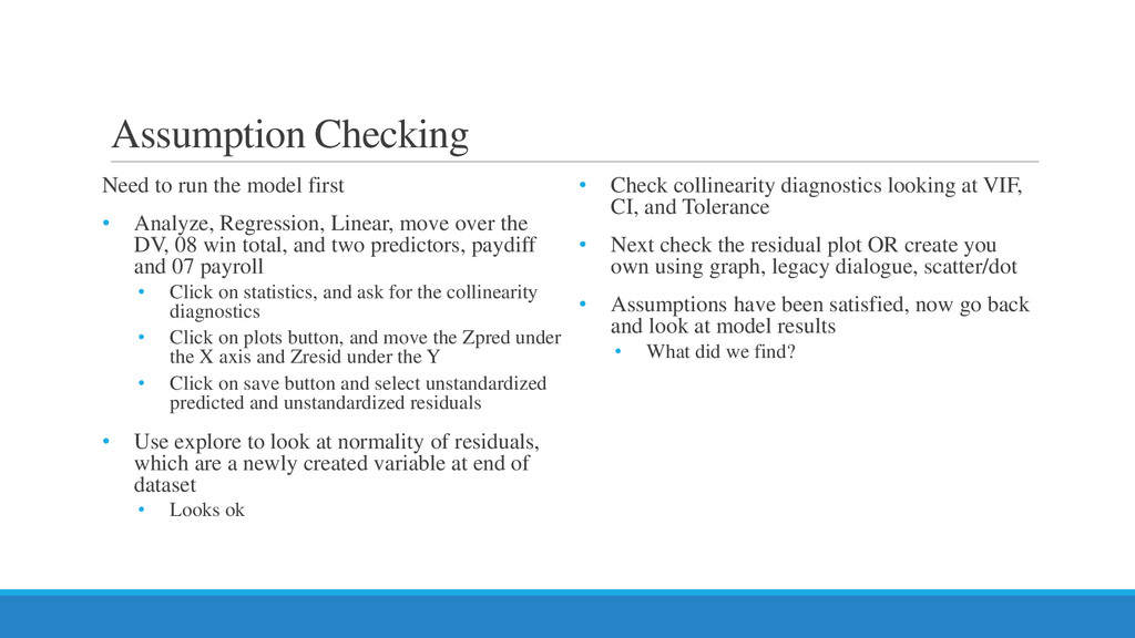
Regression, Linear, move over the DV, 08 win total, and two predictors, paydiff and 07 payroll • Click on statistics, and ask for the collinearity diagnostics • Click on plots button, and move the Zpred under the X axis and Zresid under the Y • Click on save button and select unstandardized predicted and unstandardized residuals • Use explore to look at normality of residuals, which are a newly created variable at end of dataset • Looks ok • Check collinearity diagnostics looking at VIF, CI, and Tolerance • Next check the residual plot OR create you own using graph, legacy dialogue, scatter/dot • Assumptions have been satisfied, now go back and look at model results • What did we find?
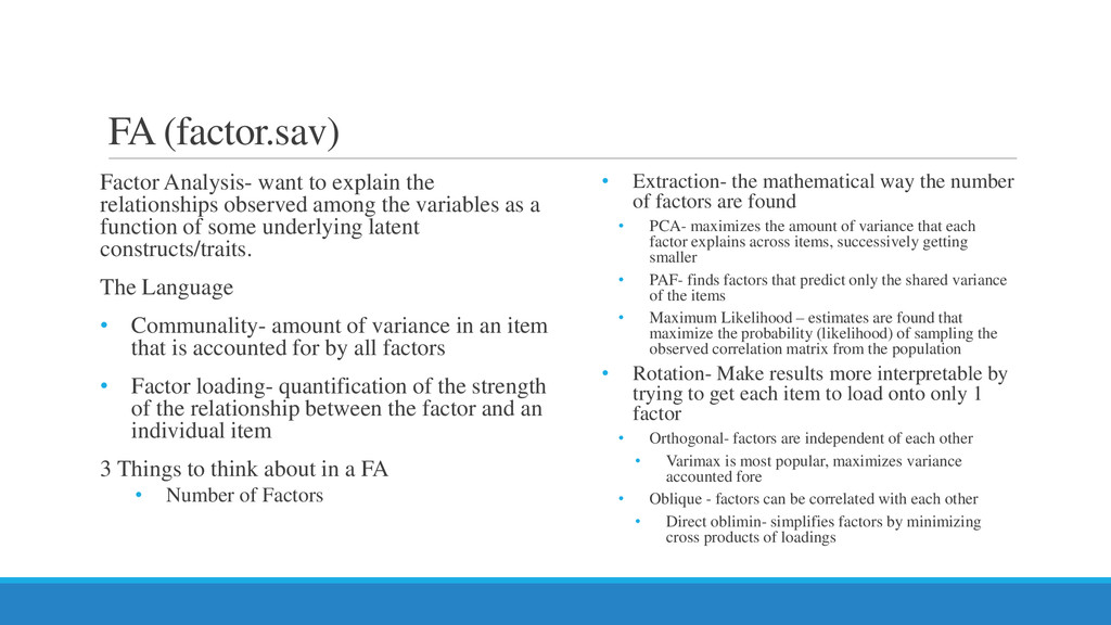
among the variables as a function of some underlying latent constructs/traits. The Language • Communality- amount of variance in an item that is accounted for by all factors • Factor loading- quantification of the strength of the relationship between the factor and an individual item 3 Things to think about in a FA • Number of Factors • Extraction- the mathematical way the number of factors are found • PCA- maximizes the amount of variance that each factor explains across items, successively getting smaller • PAF- finds factors that predict only the shared variance of the items • Maximum Likelihood – estimates are found that maximize the probability (likelihood) of sampling the observed correlation matrix from the population • Rotation- Make results more interpretable by trying to get each item to load onto only 1 factor • Orthogonal- factors are independent of each other • Varimax is most popular, maximizes variance accounted fore • Oblique - factors can be correlated with each other • Direct oblimin- simplifies factors by minimizing cross products of loadings
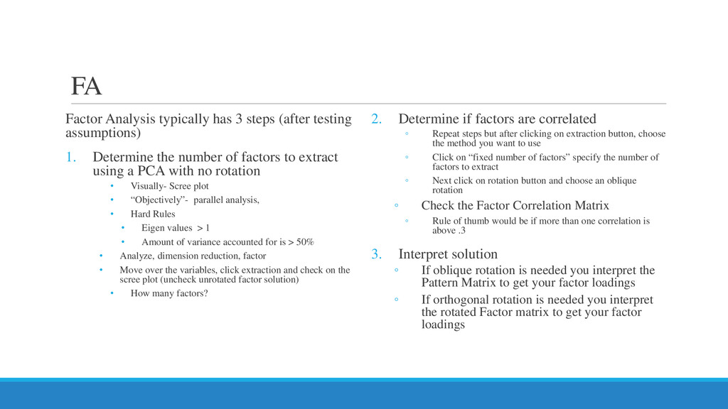
1. Determine the number of factors to extract using a PCA with no rotation • Visually- Scree plot • “Objectively”- parallel analysis, • Hard Rules • Eigen values > 1 • Amount of variance accounted for is > 50% • Analyze, dimension reduction, factor • Move over the variables, click extraction and check on the scree plot (uncheck unrotated factor solution) • How many factors? 2. Determine if factors are correlated ◦ Repeat steps but after clicking on extraction button, choose the method you want to use ◦ Click on “fixed number of factors” specify the number of factors to extract ◦ Next click on rotation button and choose an oblique rotation ◦ Check the Factor Correlation Matrix ◦ Rule of thumb would be if more than one correlation is above .3 3. Interpret solution ◦ If oblique rotation is needed you interpret the Pattern Matrix to get your factor loadings ◦ If orthogonal rotation is needed you interpret the rotated Factor matrix to get your factor loadings
reliability, select alpha from drop down, move over items • Click statistics, choose all in the “descriptives for” box and check the inter-item correlations Multiple Raters • Cohen’s kappa (Agreement for 2 raters) • Analyze, Descriptives, Crosstabs, move over the rater 1 to rows and 1 to columns • Click on statistics, choose kappa • ICC (intraclass correlation coefficient • Analyze, Scale, reliability, select alpha from drop down, move over items • Click on ICC, choose appropriate one ICC • One-Way: when raters did NOT rate all items • Two-way random: If raters rated all items, but they represent only a sample of possible raters • Two-way mixed: if raters rated all items, and represent all the raters that will be used. • This is most common for research • If the variability due to personal responding of raters is not “error” and Consistency should be chosen in the drop down on the right side.
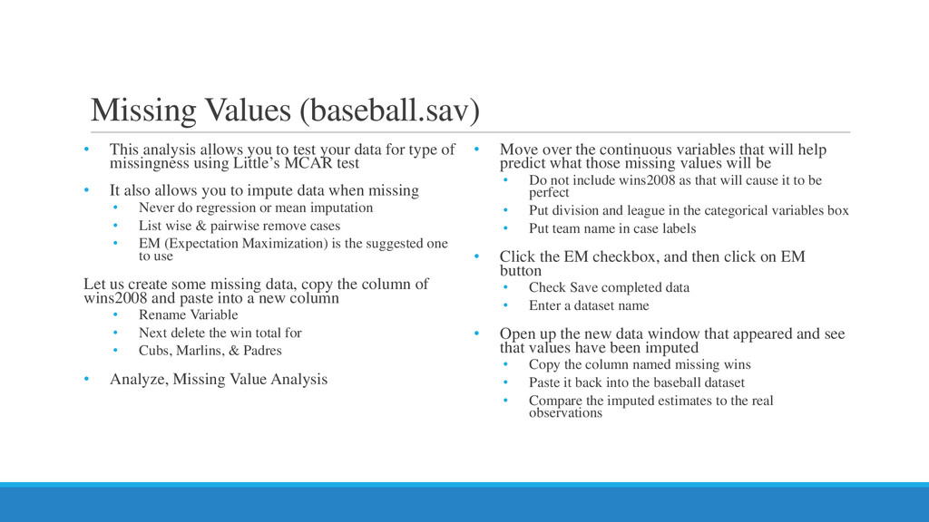
your data for type of missingness using Little’s MCAR test • It also allows you to impute data when missing • Never do regression or mean imputation • List wise & pairwise remove cases • EM (Expectation Maximization) is the suggested one to use Let us create some missing data, copy the column of wins2008 and paste into a new column • Rename Variable • Next delete the win total for • Cubs, Marlins, & Padres • Analyze, Missing Value Analysis • Move over the continuous variables that will help predict what those missing values will be • Do not include wins2008 as that will cause it to be perfect • Put division and league in the categorical variables box • Put team name in case labels • Click the EM checkbox, and then click on EM button • Check Save completed data • Enter a dataset name • Open up the new data window that appeared and see that values have been imputed • Copy the column named missing wins • Paste it back into the baseball dataset • Compare the imputed estimates to the real observations