Incremental Development Productivity Decline

by Ramin Moazeni, Barry Boehm and Daniel Link

Transcript

1. + Incremental Development Productivity Decline Ramin Moazeni, Daniel Link
2. + Introduction  Incremental development is the most common development paradigm these days  Reduces risks by allowing flexibility per increment  Incremental Development Productivity Decline (IDPD)  Based on our logical considerations and industry data, we believe there is generally a decrease in productivity between increments  The decline is due to factors such as previous-increment breakage and usage feedback, increased integration and testing effort. 10/22/2013 2 Copyright © USC-CSSE
3. + Incremental Development - Definition  Any development effort with:  More than one step  More than one released build  Each steps build on previous ones and would not be able to stand alone without the steps that came before it  Increments have to  Contribute a significant amount of new functionality  Add a significant amount of size (not less than 1/10th of the previous one)  Not just a bug fix of the previous one (otherwise counted as part of that one) 10/22/2013 3 Copyright © USC-CSSE
4. + Definitions  Build  All the code written up to a release  Increment  Only the code written between one build and the next  Any line of code is written for a given increment 10/22/2013 4 Copyright © USC-CSSE
5. + Effects of IDPD on Number of Increments  Model relating productivity decline to number of builds needed to reach 8M SLOC Full Operational Capability  Assume Build 1 production of 2M SLOC @100 SLOC/PM  20000 PM/24mo. = 833 developers  Constant Staff size for all builds 10/22/2013 5 Copyright © USC-CSSE
6. + Exploration of IDPD factor  Based on experience on several projects, the following sources of variations have been identified: 10/22/2013 6 Copyright © USC-CSSE
7. + Productivity  Conventionally:  In software development: 10/22/2013 7 Copyright © USC-CSSE
8. + IDPD type characteristics Software Category Impact on IDPD Factor Non-Deployable Throw-away code. Low Build-Build integration. High reuse. IDPD factor lowest than any type of deployable/operational software Infrastructure Software Often the most difficult software. Developed early on in the program. IDPD factor likely to be the highest. Application Software Builds upon Infrastructure software. Productivity can be increasing, or at least “flat” Platform Software Developed by HW manufacturers. Single vendor, experienced staff in a single controlled environment. Integration effort is primarily with HW. IDPD will be lower due to the benefits mentioned above. Firmware (Single Build) IDPD factor not applicable. Single build increment. 10/22/2013 8 Copyright © USC-CSSE
9. + Research Hypotheses  1) There is a decline in productivity over increments  Methods to prove  Statistically representative sample (infeasible)  Case studies that are sufficiently general  Data sources  Data from experience/history  Controlled experiments  Model Fitting  F-Test  Linear Correlation  2) Decline is not always constant for all incrementally developed projects  T-Test  3) Decline varies by domain  Can be proven by statistics (ANOVA) 10/22/2013 9 Copyright © USC-CSSE
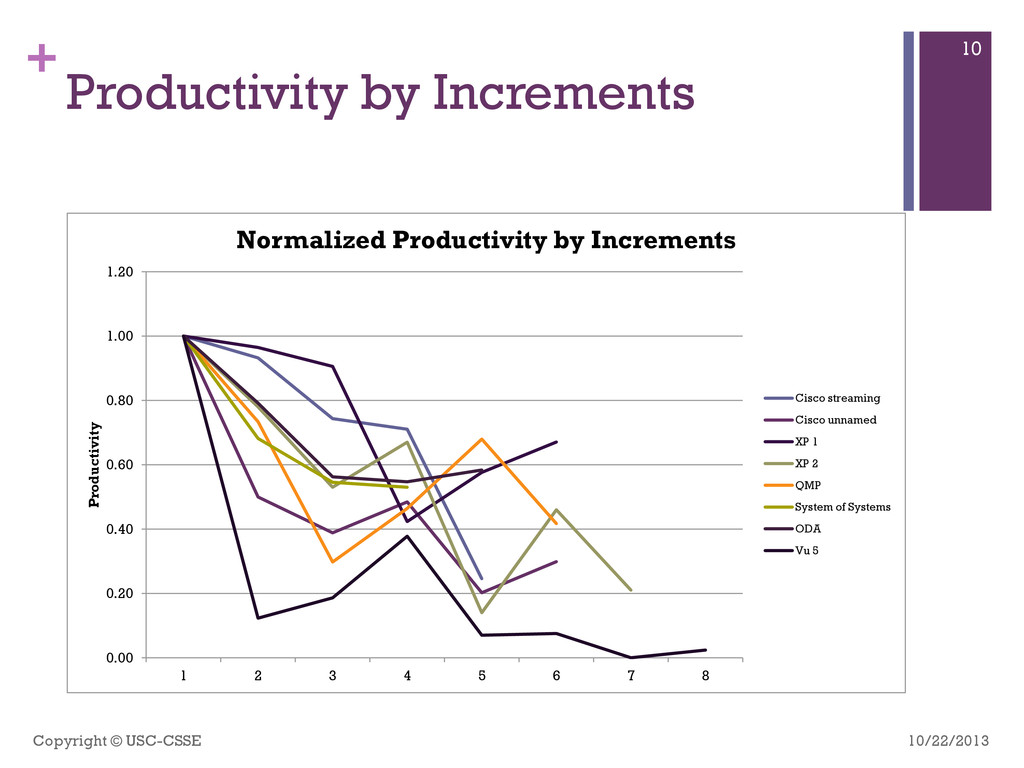
10. + Productivity by Increments 10/22/2013 10 Copyright © USC-CSSE 0.00 0.20 0.40 0.60 0.80 1.00 1.20 1 2 3 4 5 6 7 8 Productivity Normalized Productivity by Increments Cisco streaming Cisco unnamed XP 1 XP 2 QMP System of Systems ODA Vu 5
11. + Polynomial trend line 0.85 0.82 0.77 0.36 0.49 0.57 y = -0.023x5 + 0.3966x4 - 2.5291x3 + 7.321x2 - 9.5311x + 5.2174 R² = 1 0.00 0.10 0.20 0.30 0.40 0.50 0.60 0.70 0.80 0.90 1.00 1 2 3 4 5 6 New Development Effort of Project 1 Project 1 Poly. (Project 1) 10/22/2013 11 Copyright © USC-CSSE
12. + Polynomial trend line (continued) 0.85 0.82 0.77 0.36 0.49 0.57 y = -0.023x5 + 0.3966x4 - 2.5291x3 + 7.321x2 - 9.5311x + 5.2174 R² = 1 -5.00 -4.00 -3.00 -2.00 -1.00 0.00 1.00 2.00 1 2 3 4 5 6 7 New Development Effort of Project 1 Project 1 Poly. (Project 1) 10/22/2013 12 Copyright © USC-CSSE
13. + Comparison of trend lines 0.85 0.82 0.77 0.36 0.49 0.57 y = -0.233ln(x) + 0.8975 R² = 0.6012 y = 0.9445e-0.124x R² = 0.4563 y = 0.9141x-0.364 R² = 0.4982 0.00 0.10 0.20 0.30 0.40 0.50 0.60 0.70 0.80 0.90 1.00 1 2 3 4 5 6 New Development Efforts of Project 1 Project 1 Log. (Project 1) Expon. (Project 1) Power (Project 1) 10/22/2013 13 Copyright © USC-CSSE
14. + Comparison of trend lines (continued) 1.00 0.78 0.53 0.67 0.14 0.46 0.21 y = -0.392ln(x) + 1.0218 R² = 0.7731 y = 1.175x-0.782 R² = 0.5687 y = 1.2393e-0.251x R² = 0.585 0.00 0.20 0.40 0.60 0.80 1.00 1.20 1.40 1 2 3 4 5 6 7 New Development Efforts of Project 2 Project 2 Log. (Project 2) Power (Project 2) Expon. (Project 2) 10/22/2013 14 Copyright © USC-CSSE
15. + Comparison of trend lines (continued) 10/22/2013 15 Copyright © USC-CSSE y = -0.7989x + 8.5493 R² = 0.3693 y = -2.708ln(x) + 8.7233 R² = 0.5326 0 2 4 6 8 10 12 1 2 3 4 5 6 QMP Productivity Linear (Productivity) Log. (Productivity)
16. + Trend line summary  Logarithmic is best fit in most observed real-world cases  Trend line alone is not enough for reasonably precise prediction of effort for next increment  => Additional predictors needed  Additionally, we have 22 COCOMO II cost drivers that all can influence the decline for the next given increment. Examples: Complexity (CPLX), Personnel Continuity (PCON), Reliability (RELY), Architectural Resolution (RESL). 10/22/2013 16 Copyright © USC-CSSE
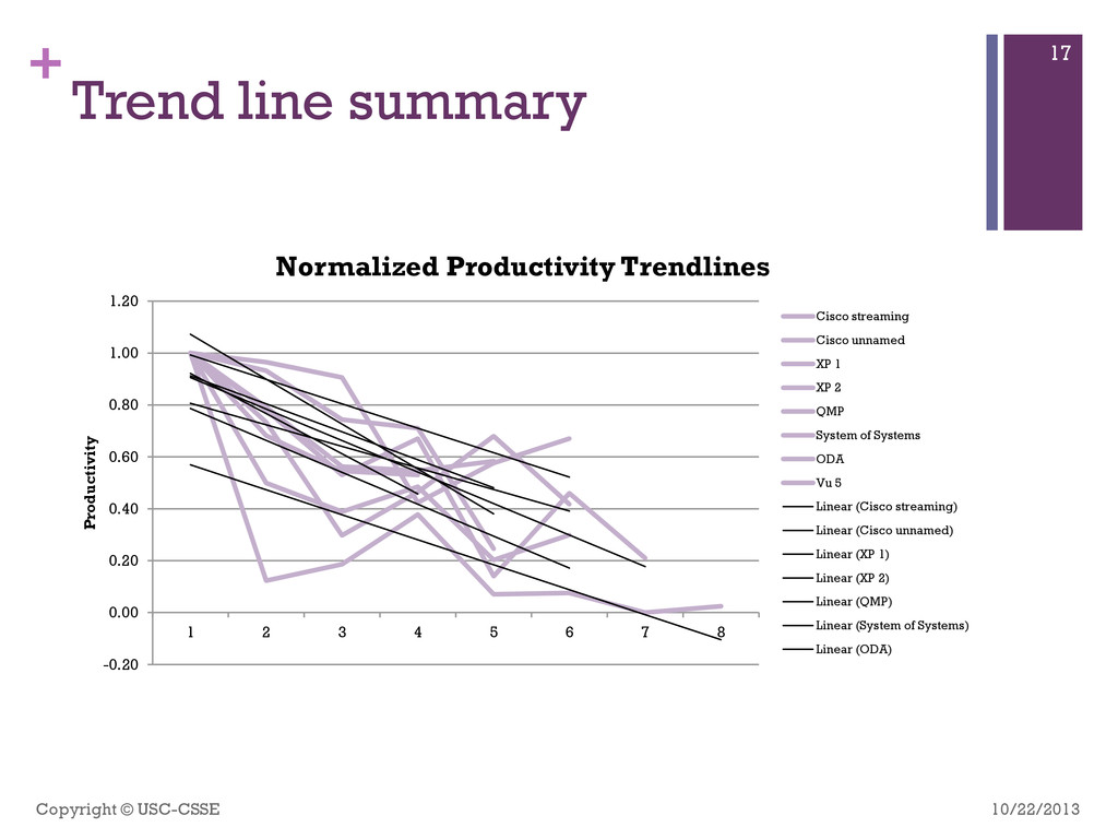
17. + Trend line summary 10/22/2013 17 Copyright © USC-CSSE -0.20 0.00 0.20 0.40 0.60 0.80 1.00 1.20 1 2 3 4 5 6 7 8 Productivity Normalized Productivity Trendlines Cisco streaming Cisco unnamed XP 1 XP 2 QMP System of Systems ODA Vu 5 Linear (Cisco streaming) Linear (Cisco unnamed) Linear (XP 1) Linear (XP 2) Linear (QMP) Linear (System of Systems) Linear (ODA)
18. + F-Test & Correlation 10/22/2013 18 Copyright © USC-CSSE Project P-Value Correlation Coefficient 1 0.024 -0.92645290 2 0.044 -0.82426625 3 0.086 -0.74995815 4 0.014 -0.85749292 5 0.057 -0.86750112 6 0.201 -0.60769380 7 0.085 -0.91524923 8 0.151 -0.70972771
19. + Regression Weighted by Size  Looking at the Regression weighted by the size of increments 10/22/2013 19 Copyright © USC-CSSE Project P-Value R-Square 1 0.024 85.70% 2 0.015 81% 3 0.086 56.20% 4 0.014 73.50% 5 0.067 72.40% 6 0.141 45.60% 7 0.085 83.70% 8 0.019 69.70%
20. + Case study  Quality Management Project (QMP)  Web-based application  System is to facilitate the process improvement initiatives in many small and medium software organizations  6 builds, 6 years, different increment duration  Size after 6th build: 548 KSLOC mostly in Java  Average staff on project: ~20 10/22/2013 20 Copyright © USC-CSSE
21. + Quality Management Platform (QMP) Project 10/22/2013 21 Copyright © USC-CSSE
22. + Conclusions and outlook  More data with detailed back stories needs to be collected  Controlled experiment with artificial events  Already completed.  Use IDPD model to extend COCOMO II  Expert judgments / workshops 10/22/2013 22 Copyright © USC-CSSE
23. + Hofstadter's law  Hofstadter's Law: It always takes longer than you expect, even when you take into account Hofstadter's Law. — Douglas Hofstadter 10/22/2013 Copyright © USC-CSSE 23
24. +