Exploring aerospace design in virtual reality with dimension reduction

Slides from my talk at AIAA Scitech 2019, San Diego, CA.

Transcript

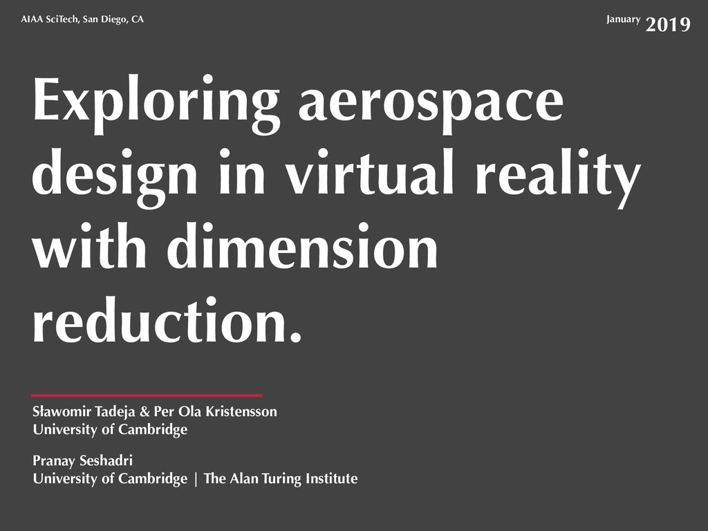
1. Exploring aerospace design in virtual reality with dimension reduction. AIAA SciTech, San Diego, CA January 2019 Pranay Seshadri University of Cambridge | The Alan Turing Institute Sławomir Tadeja & Per Ola Kristensson University of Cambridge
2. Sławomir Konrad Tadeja PhD Student in Virtual Reality, Intelligent Interactive Systems Lab, University of Cambridge https://skt40.github.io Per Ola Kristensson Professor and Director, Intelligent Interactive Systems Lab, University of Cambridge
3. Exploring aerospace design in virtual reality with dimension reduction. A complex multi-discplinary, multi- objective and high-dimensional problem. Technologies that facilitate faster design cycle times can be real game changers.
4. Exploring aerospace design in virtual reality with dimension reduction. noun. A realistic and immersive simulation of a three-dimensional environment, created using interactive software and hardware, and experienced or controlled by movement of the body. [vur-choo-uh l ree-al-i-tee]
5. Exploring aerospace design in virtual reality with dimension reduction. [Above] An engineer suffering from the curse of dimensionality.
6. Overview. Sufficient summary plots Virtual reality (VR) Leveraging VR for design studies
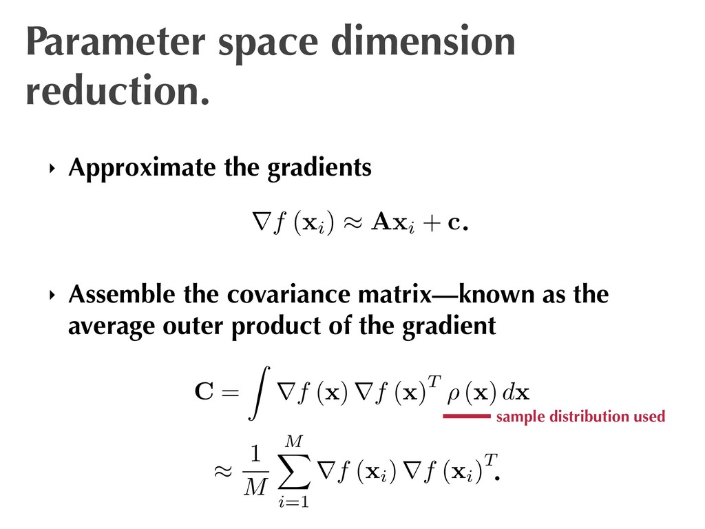
7. Sufficient summary plots. ‣ Aerospace design demands the exploration of high- dimensional spaces. ‣ Challenging to visualize high-dimensional spaces. ‣ We wish to visualize key output quantities of interest as functions of input parameters. ‣ Can utilize ideas from dimension reduction to aid this endeavor.
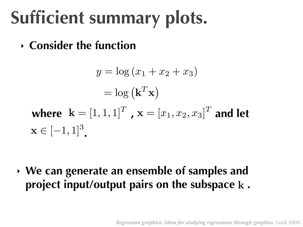
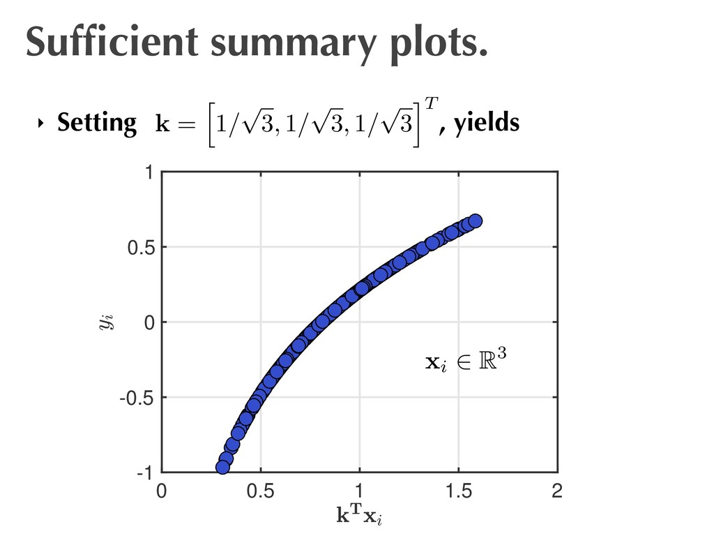
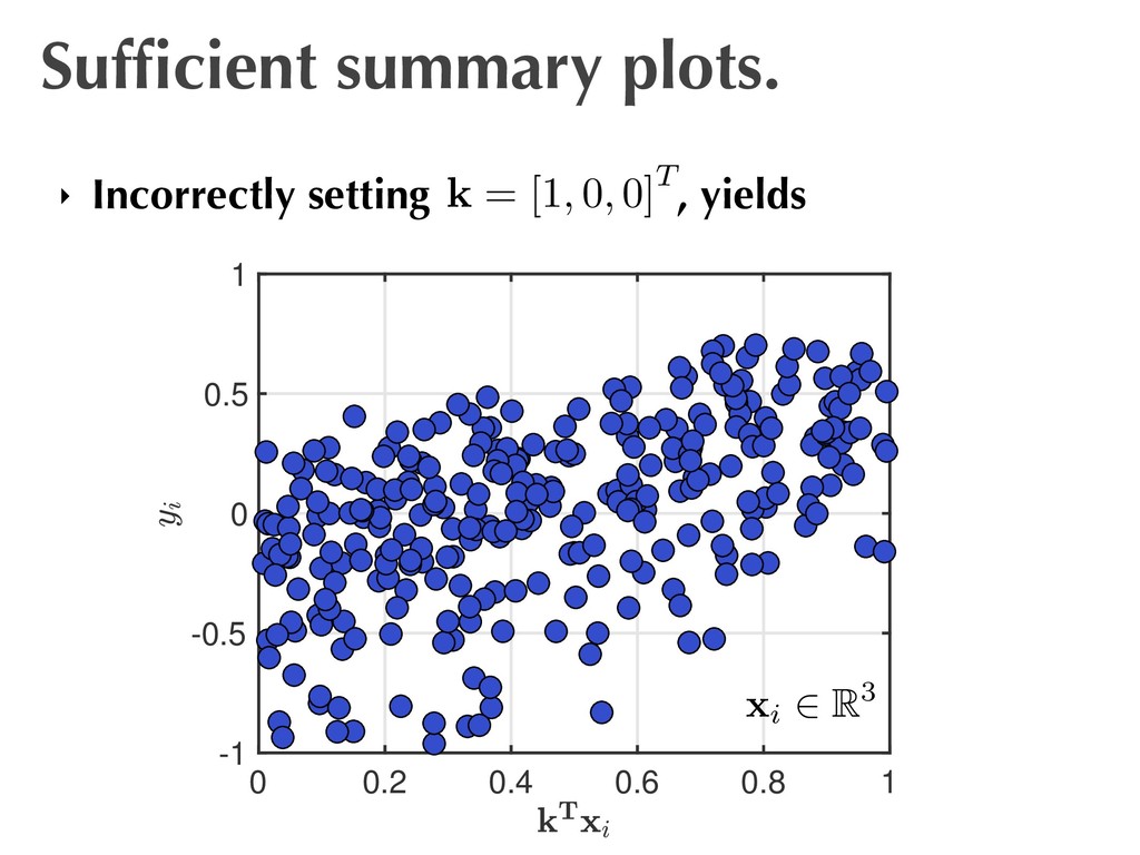
8. Sufficient summary plots. ‣ Consider the function y = log (x1 + x2 + x3) y = log kT x k = [1, 1, 1]T where , and let x 2 [ 1, 1]3 ‣ We can generate an ensemble of samples and project input/output pairs on the subspace . k x = [x1, x2, x3]T . Regression graphics: Ideas for studying regressions through graphics. Cook 2009.
9. Sufficient summary plots. 0 0.5 1 1.5 2 -1 -0.5 0 0.5 1 ‣ Setting , yields k = h 1/ p 3, 1/ p 3, 1/ p 3 iT xi 2 R3
10. Sufficient summary plots. ‣ Incorrectly setting , yields k = [1, 0, 0]T 0 0.2 0.4 0.6 0.8 1 -1 -0.5 0 0.5 1 xi 2 R3
11. Sufficient summary plots. ‣ Incorrectly setting , yields k = [0.2, 0.5, 0.2]T 0 0.2 0.4 0.6 0.8 1 -1 -0.5 0 0.5 1 xi 2 R3
12. Sufficient summary plots. ‣ The key computational challenge is identifying using few input/output pairs—for “real-world” aerospace models. k
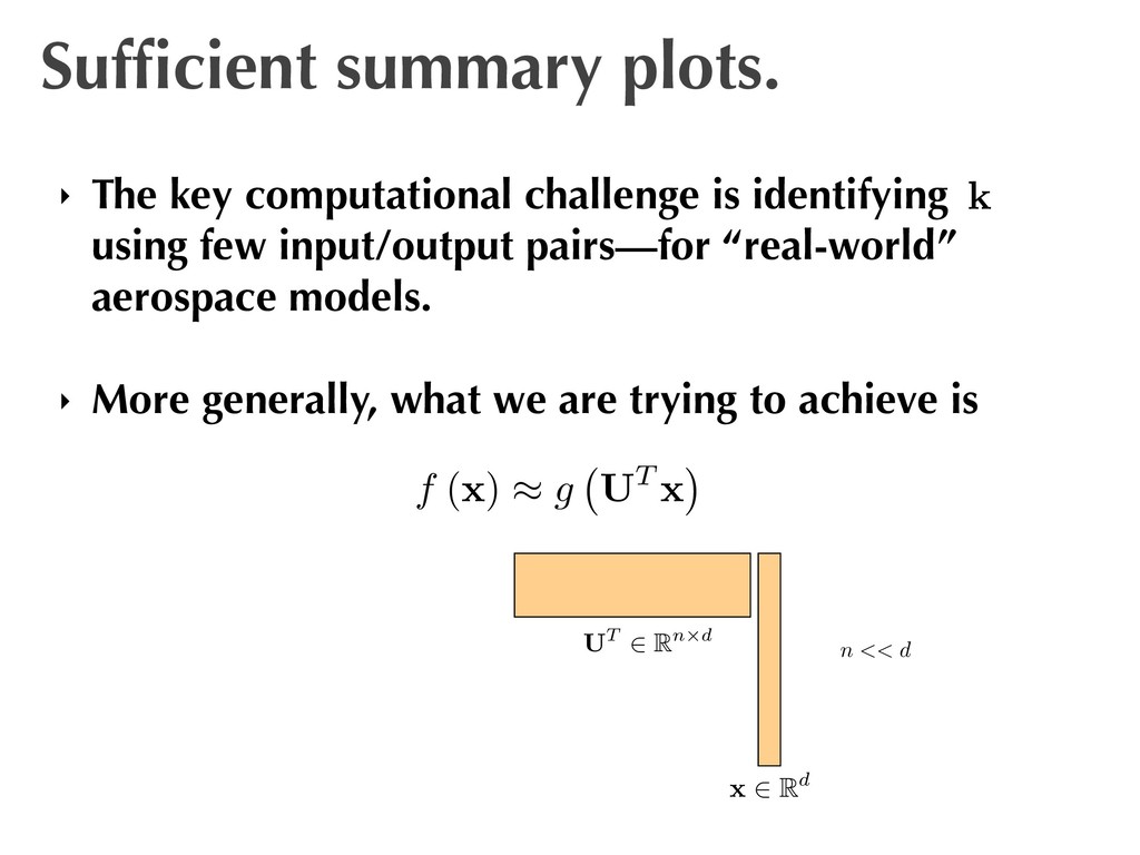
13. Sufficient summary plots. ‣ The key computational challenge is identifying using few input/output pairs—for “real-world” aerospace models. ‣ More generally, what we are trying to achieve is k f (x) ⇡ g UT x UT 2 Rn⇥d x 2 Rd n << d
14. Sufficient summary plots. ‣ There has been an explosion of work in this area from different communities. ‣ Resulting in numerous recipes to achieve the approximation f (x) ⇡ g UT x .
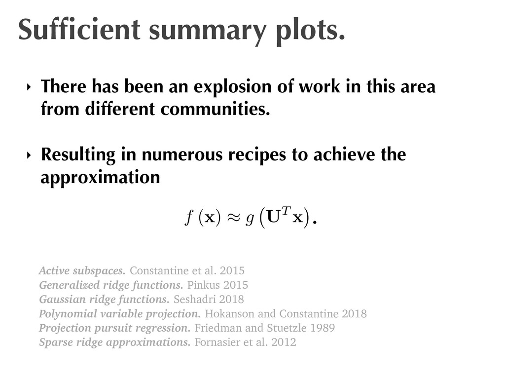
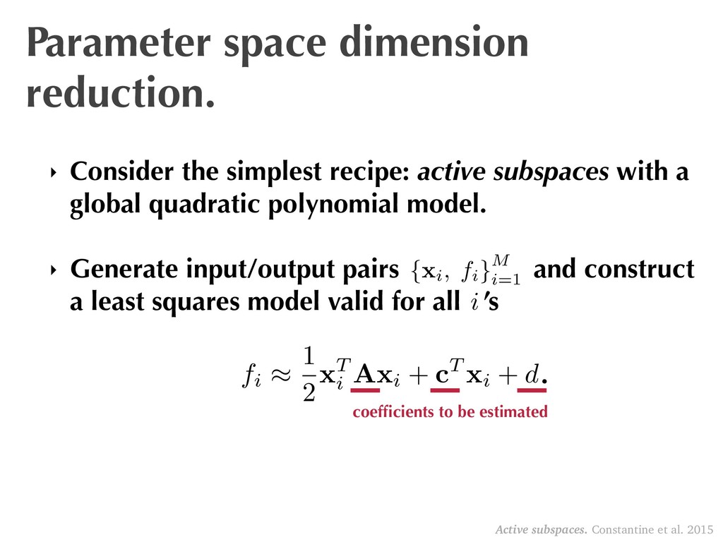
15. Sufficient summary plots. ‣ There has been an explosion of work in this area from different communities. ‣ Resulting in numerous recipes to achieve the approximation f (x) ⇡ g UT x Active subspaces. Constantine et al. 2015 Generalized ridge functions. Pinkus 2015 Gaussian ridge functions. Seshadri 2018 Polynomial variable projection. Hokanson and Constantine 2018 Projection pursuit regression. Friedman and Stuetzle 1989 Sparse ridge approximations. Fornasier et al. 2012 .
16. Parameter space dimension reduction. ‣ Consider the simplest recipe: active subspaces with a global quadratic polynomial model. Active subspaces. Constantine et al. 2015
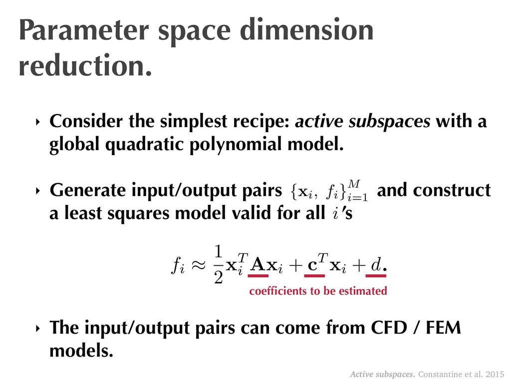
17. Parameter space dimension reduction. ‣ Consider the simplest recipe: active subspaces with a global quadratic polynomial model. ‣ Generate input/output pairs and construct a least squares model valid for all ’s {xi, fi }M i=1 fi ⇡ 1 2 xT i Axi + cT xi + d coefficients to be estimated i . Active subspaces. Constantine et al. 2015
18. Parameter space dimension reduction. ‣ Consider the simplest recipe: active subspaces with a global quadratic polynomial model. ‣ Generate input/output pairs and construct a least squares model valid for all ’s ‣ The input/output pairs can come from CFD / FEM models. {xi, fi }M i=1 fi ⇡ 1 2 xT i Axi + cT xi + d coefficients to be estimated i . Active subspaces. Constantine et al. 2015
19. Parameter space dimension reduction. ‣ Approximate the gradients rf (xi) ⇡ Axi + c.
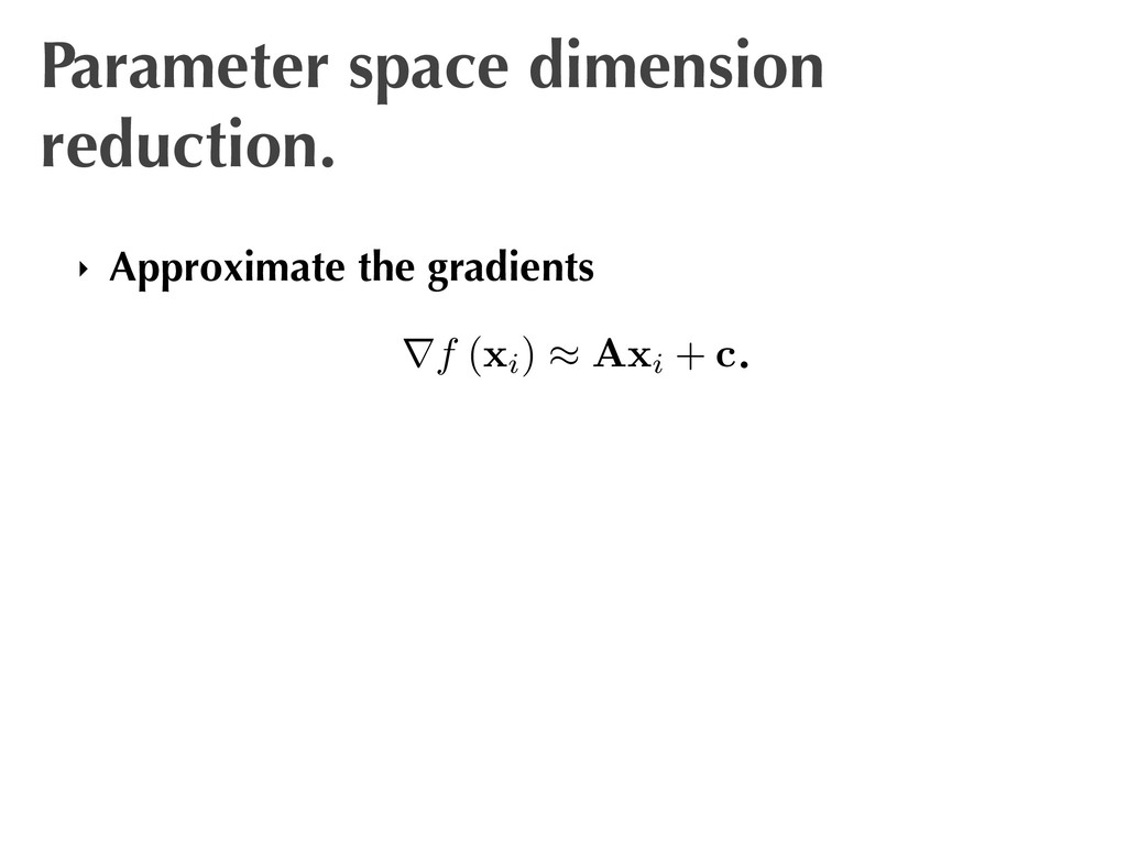
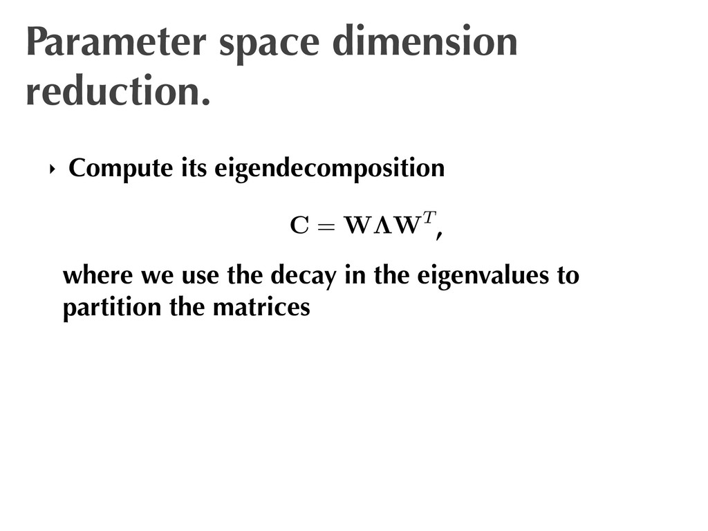
20. Parameter space dimension reduction. ‣ Approximate the gradients ‣ Assemble the covariance matrix—known as the average outer product of the gradient rf (xi) ⇡ Axi + c. sample distribution used ⇡ 1 M M X i=1 rf (xi) rf (xi)T. C = Z rf (x) rf (x)T ⇢ (x) dx
21. Parameter space dimension reduction. ‣ Compute its eigendecomposition C = W⇤WT where we use the decay in the eigenvalues to partition the matrices ,
22. Parameter space dimension reduction. ‣ Compute its eigendecomposition C = W⇤WT where we use the decay in the eigenvalues to partition the matrices W = ⇥ W1 W2 ⇤ , ⇤ =  ⇤1 ⇤2 , . ‣ Finally, use the subspace for U = W1 f (x) ⇡ g UT x . Note: This is not principal components analysis!
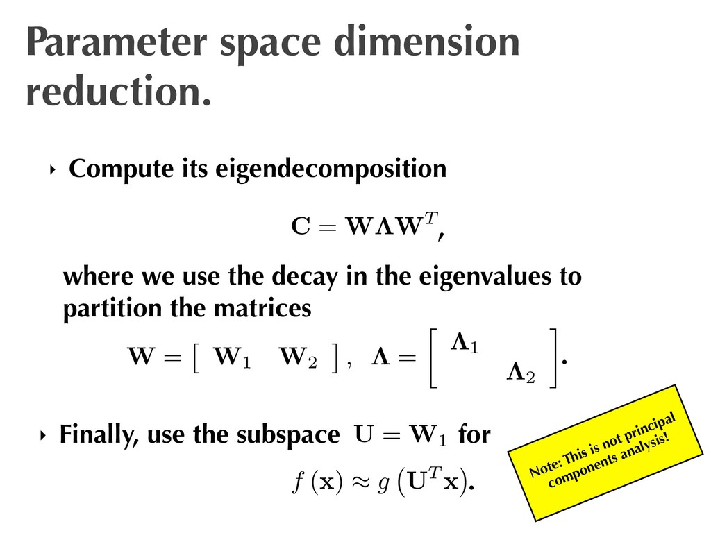
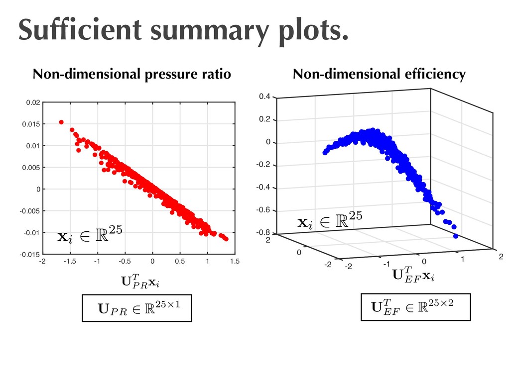
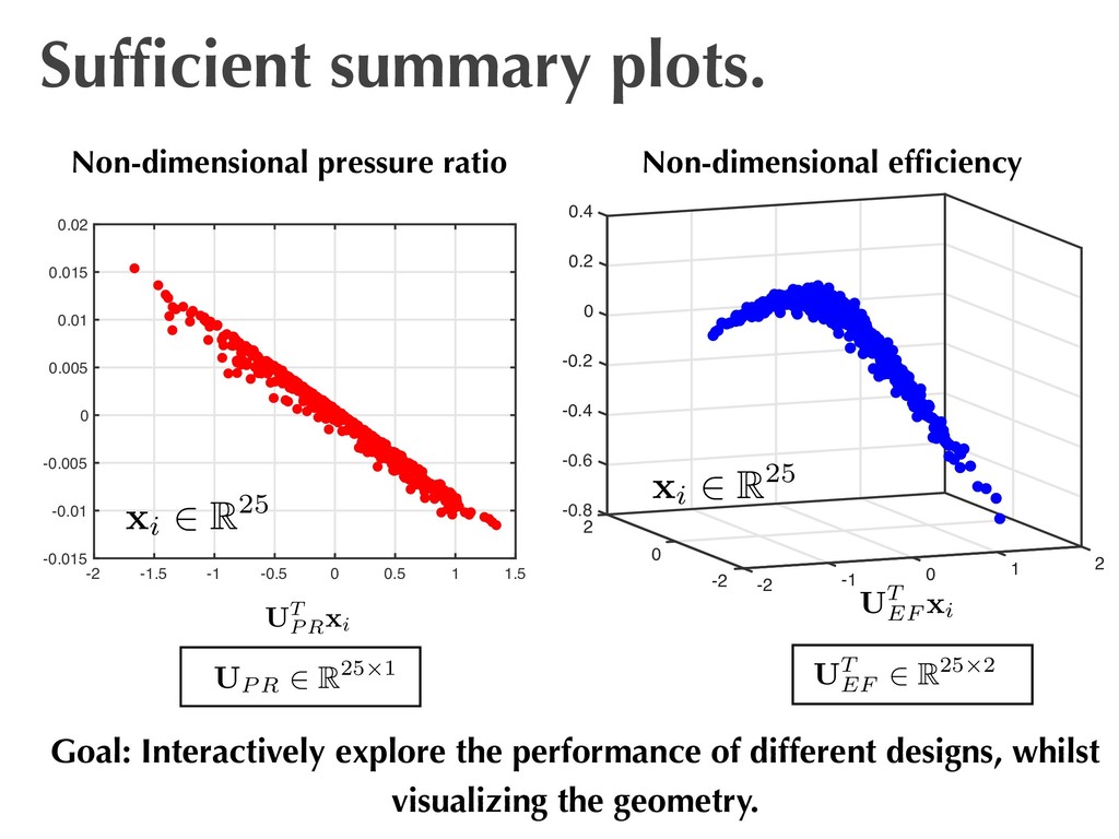
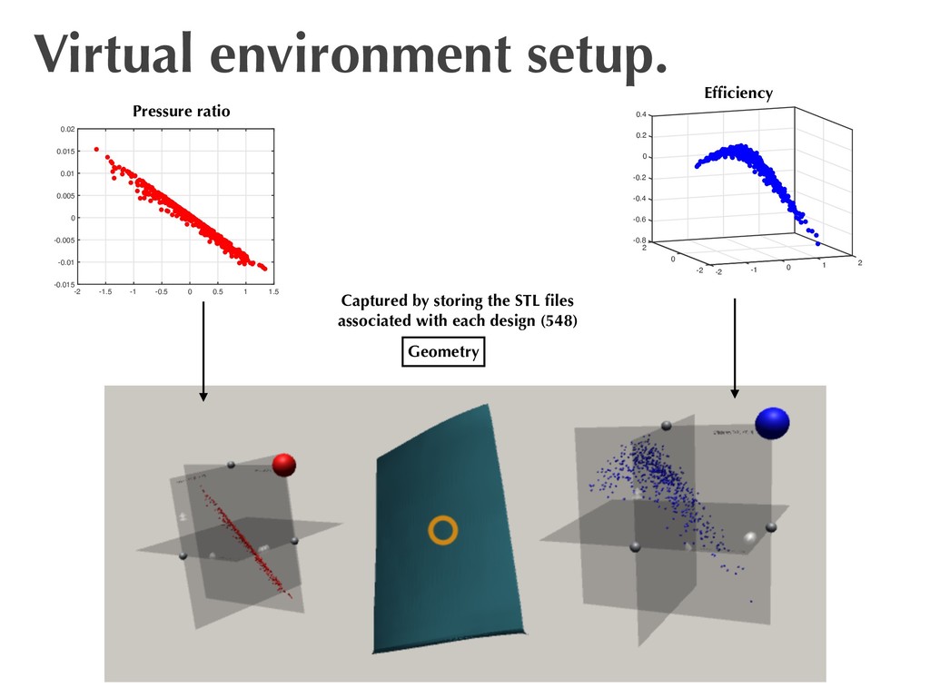
23. Aerospace design application. ‣ Previously applied this recipe to a compressor blade. ‣ Setup Turbomachinery active subspace performance maps. Seshadri, Shahpar, Constantine, Parks, Adams 2018. x 2 R25 Design space of 3D blade parameters with 25 design variables Wish to study efficiency and pressure-ratio objectives ⌘, PR Input/output pairs generated by evaluating CFD on a Latin Hypercube DOE M = 548
24. Sufficient summary plots. -2 -1.5 -1 -0.5 0 0.5 1 1.5 -0.015 -0.01 -0.005 0 0.005 0.01 0.015 0.02 xi 2 R25 -0.8 -0.6 -0.4 -0.2 2 0 0.2 0.4 0 2 1 0 -1 -2 -2 xi 2 R25 Non-dimensional efficiency Non-dimensional pressure ratio UT P R xi UP R 2 R25⇥1 UT EF 2 R25⇥2 UT EF xi
25. Sufficient summary plots. -2 -1.5 -1 -0.5 0 0.5 1 1.5 -0.015 -0.01 -0.005 0 0.005 0.01 0.015 0.02 xi 2 R25 -0.8 -0.6 -0.4 -0.2 2 0 0.2 0.4 0 2 1 0 -1 -2 -2 xi 2 R25 Non-dimensional efficiency Non-dimensional pressure ratio UT P R xi UP R 2 R25⇥1 UT EF 2 R25⇥2 UT EF xi Goal: Interactively explore the performance of different designs, whilst visualizing the geometry.
26. Overview. Sufficient summary plots Virtual reality (VR) Leveraging VR for design studies
27. Oculus Rift Oculus Go All images from Wikipedia / CC BY-SA 2.0 and 4.0 Samsung Gear PlayStation VR HTC Vive Humphries and McGreevy, NASA Ames. Virtual reality hardware.
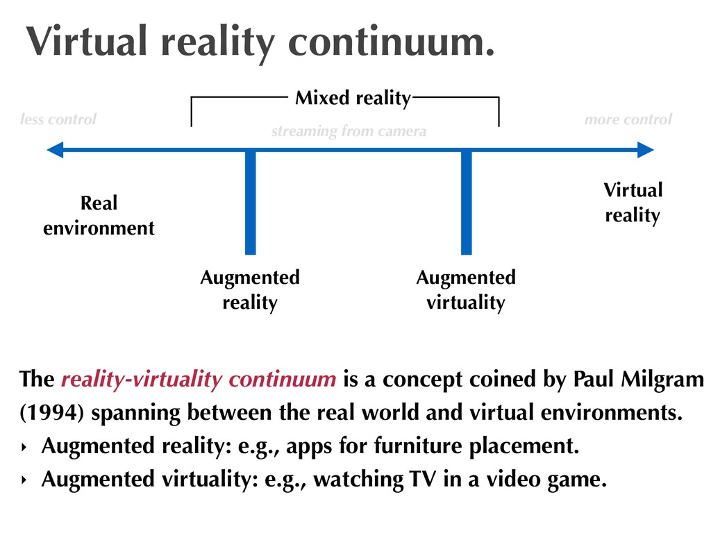
28. Virtual reality continuum. Real environment Augmented reality Augmented virtuality Virtual reality Mixed reality The reality-virtuality continuum is a concept coined by Paul Milgram (1994) spanning between the real world and virtual environments. ‣ Augmented reality: e.g., apps for furniture placement. ‣ Augmented virtuality: e.g., watching TV in a video game. streaming from camera more control less control
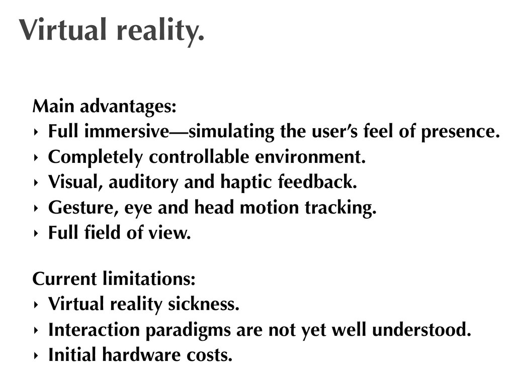
29. Virtual reality. Main advantages: ‣ Full immersive—simulating the user’s feel of presence. ‣ Completely controllable environment. ‣ Visual, auditory and haptic feedback. ‣ Gesture, eye and head motion tracking. ‣ Full field of view. Current limitations: ‣ Virtual reality sickness. ‣ Interaction paradigms are not yet well understood. ‣ Initial hardware costs.
30. Virtual reality hardware. In this study we used: ‣ a Xbox game controller; ‣ an Oculus rift motion sensor; ‣ an Oculus rift VR headset; ‣ the Unity3D framework.
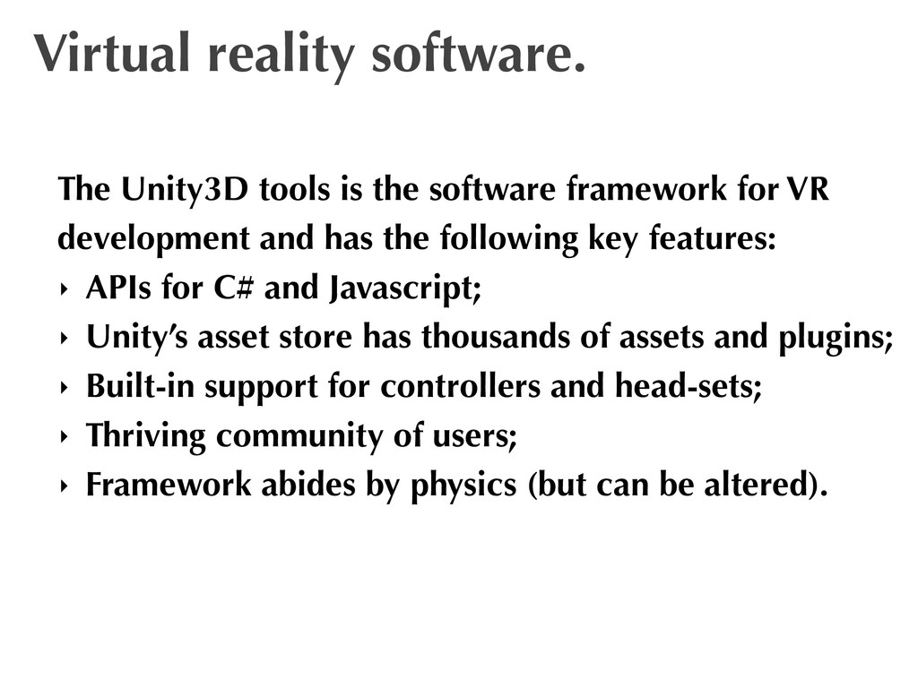
31. Virtual reality software. The Unity3D tools is the software framework for VR development and has the following key features: ‣ APIs for C# and Javascript; ‣ Unity’s asset store has thousands of assets and plugins; ‣ Built-in support for controllers and head-sets; ‣ Thriving community of users; ‣ Framework abides by physics (but can be altered).
32. Overview. Sufficient summary plots Virtual reality (VR) Leveraging VR for design studies
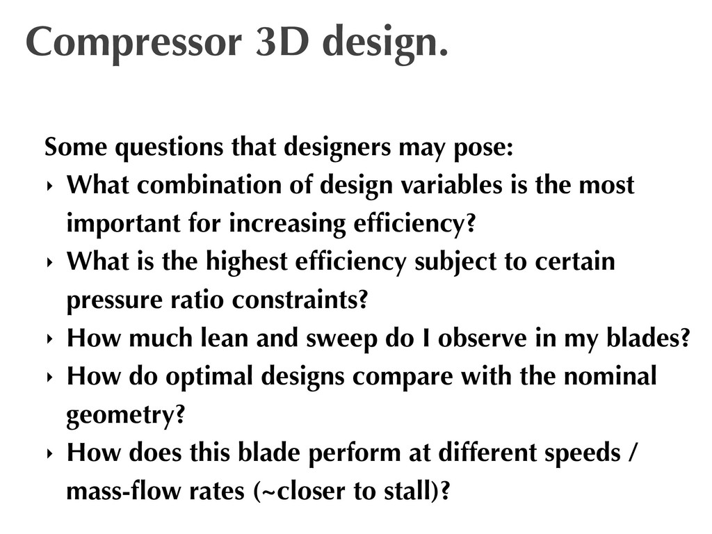
33. Compressor 3D design. Some questions that designers may pose: ‣ What combination of design variables is the most important for increasing efficiency? ‣ What is the highest efficiency subject to certain pressure ratio constraints? ‣ How much lean and sweep do I observe in my blades? ‣ How do optimal designs compare with the nominal geometry? ‣ How does this blade perform at different speeds / mass-flow rates (~closer to stall)?
34. Virtual environment setup. -2 -1.5 -1 -0.5 0 0.5 1 1.5 -0.015 -0.01 -0.005 0 0.005 0.01 0.015 0.02 -0.8 -0.6 -0.4 -0.2 2 0 0.2 0.4 0 2 1 0 -1 -2 -2 Pressure ratio Efficiency Geometry Captured by storing the STL files associated with each design (548)
35. [Right] An engineer studying the design space (two objectives) of a blade with 25 variables. [Above] What the engineer visualizes.
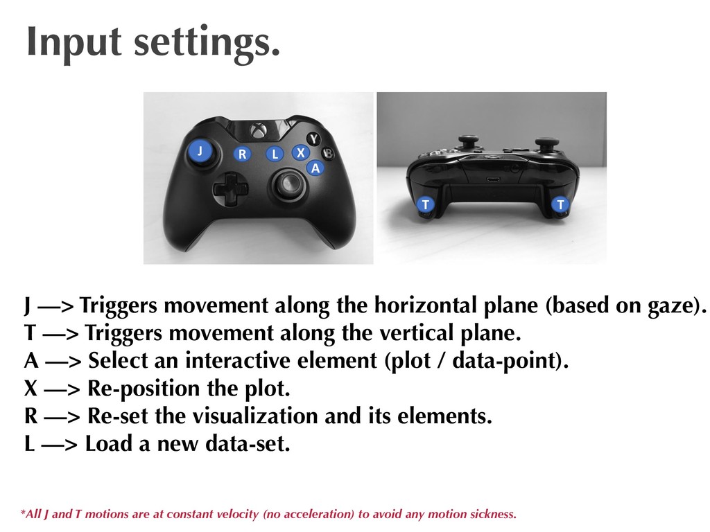
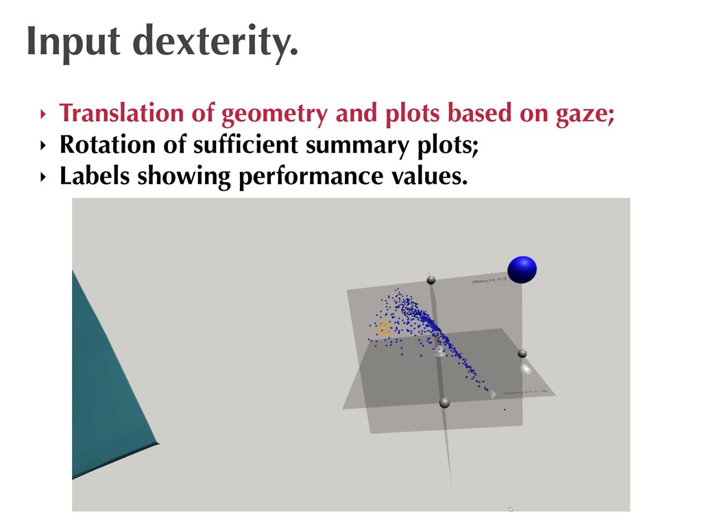
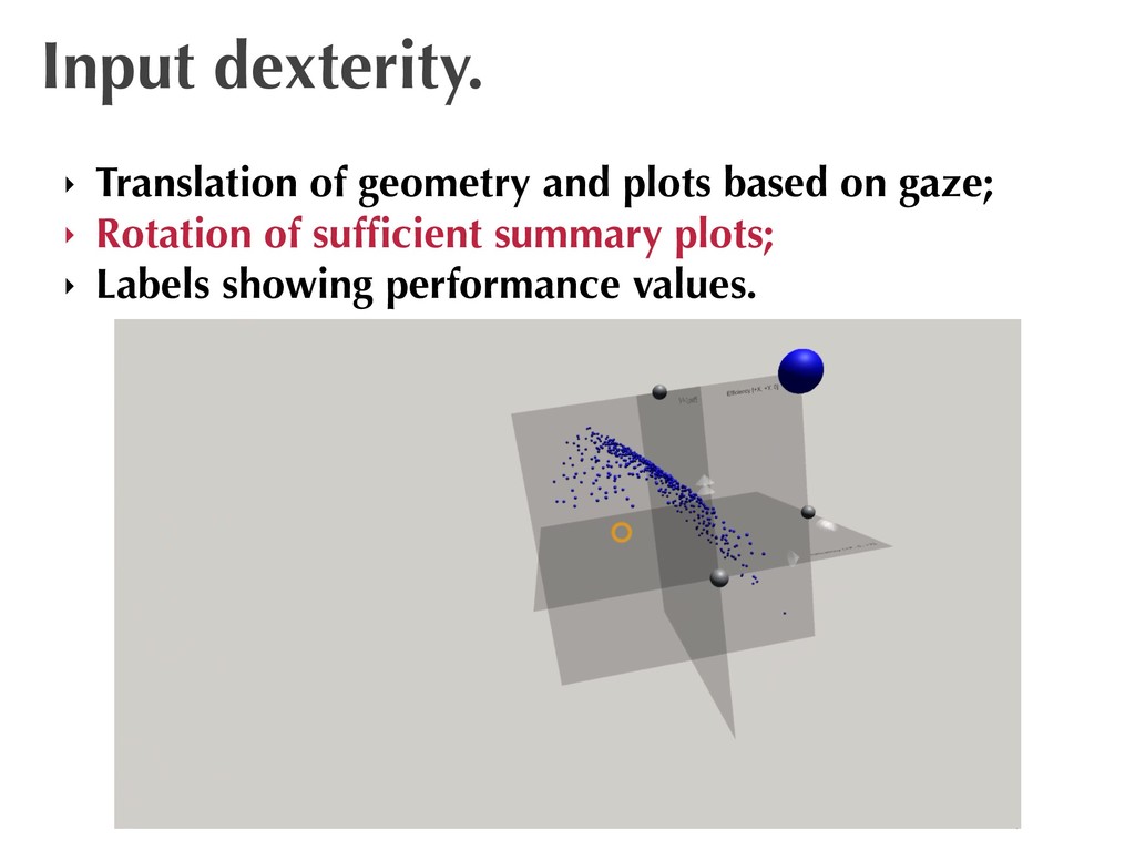
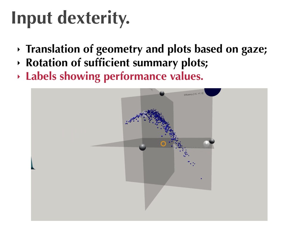
36. Input settings. T (b) J (a) T A X L R J —> Triggers movement along the horizontal plane (based on gaze). T —> Triggers movement along the vertical plane. A —> Select an interactive element (plot / data-point). X —> Re-position the plot. R —> Re-set the visualization and its elements. L —> Load a new data-set. *All J and T motions are at constant velocity (no acceleration) to avoid any motion sickness.
37. Input dexterity. ‣ Translation of geometry and plots based on gaze; ‣ Rotation of sufficient summary plots; ‣ Labels showing performance values.
38. Input dexterity. ‣ Translation of geometry and plots based on gaze; ‣ Rotation of sufficient summary plots; ‣ Labels showing performance values.
39. Input dexterity. ‣ Translation of geometry and plots based on gaze; ‣ Rotation of sufficient summary plots; ‣ Labels showing performance values.
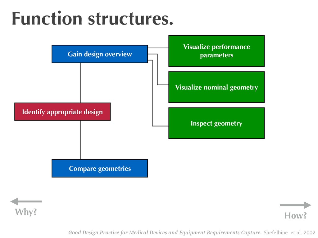
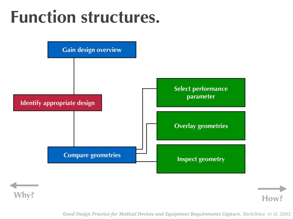
40. Function structures. Gain design overview Compare geometries Identify appropriate design Visualize performance parameters Visualize nominal geometry Inspect geometry Good Design Practice for Medical Devices and Equipment Requirements Capture. Shefelbine et al. 2002 Why? How?
41. Gain design overview Identify appropriate design Good Design Practice for Medical Devices and Equipment Requirements Capture. Shefelbine et al. 2002 Why? How? Compare geometries Select performance parameter Overlay geometries Inspect geometry Function structures.
42. Next steps. While this is a promising start, a lot more needs to be done: ‣ Custom characteristics for each design; ‣ Greater geometry detail; ‣ Visualization of constraints on sufficient summary plots; ‣ Fitting response surfaces to generate new designs on the fly (challenging because the inverse map is not unique!) ‣ User design studies and tasks with aero-designers.
43. Thank you! Sławomir Tadeja University of Cambridge skt40@cam.ac.uk