Cambridge (joint w/ Geoff Parks) James Gross PhD Research Student, Department of Engineering University of Cambridge (joint w/ Geoff Parks) Ashley Scillitoe Research Associate, The Alan Turing Institute. Słaowmir Tadeja PhD Research Student, Department of Engineering, University of Cambridge (joint w/ Per Ola Kristensson) Group members
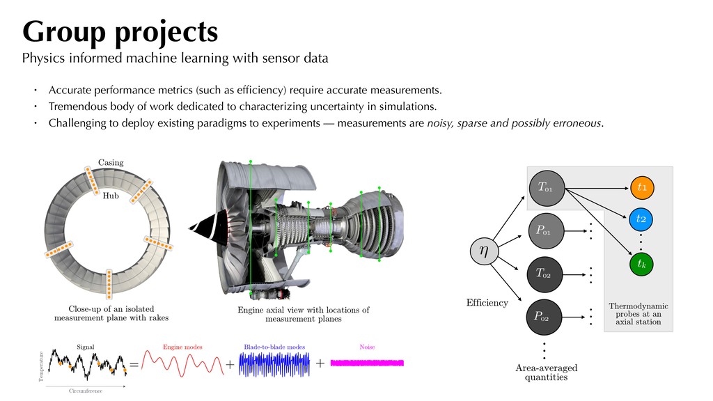
Accurate performance metrics (such as efficiency) require accurate measurements. • Tremendous body of work dedicated to characterizing uncertainty in simulations. • Challenging to deploy existing paradigms to experiments — measurements are noisy, sparse and possibly erroneous.
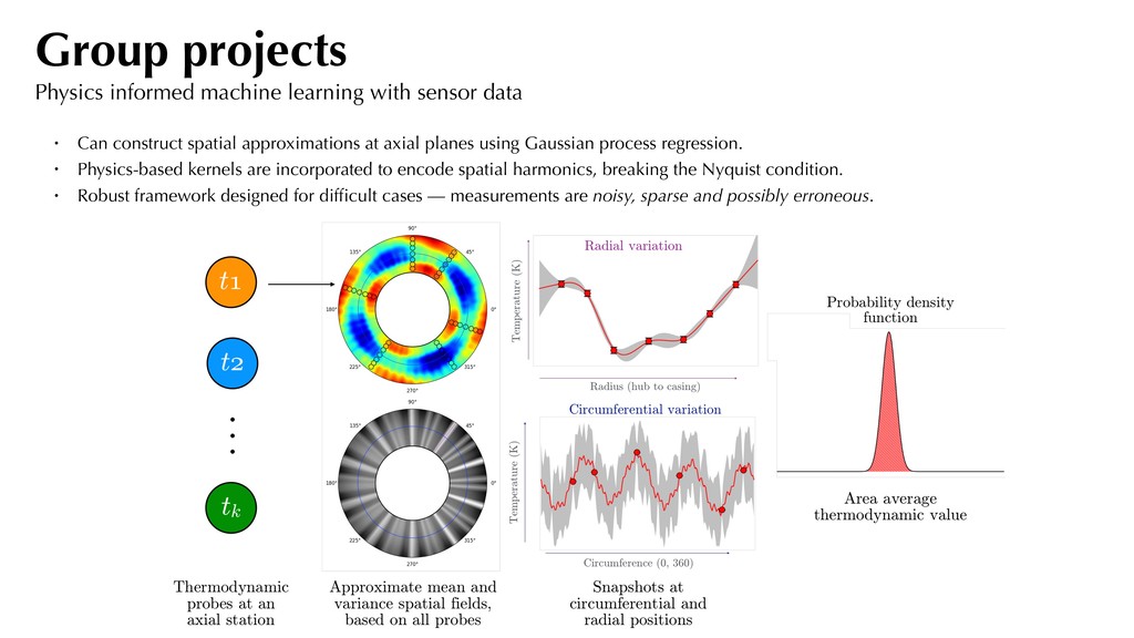
Can construct spatial approximations at axial planes using Gaussian process regression. • Physics-based kernels are incorporated to encode spatial harmonics, breaking the Nyquist condition. • Robust framework designed for difficult cases — measurements are noisy, sparse and possibly erroneous.
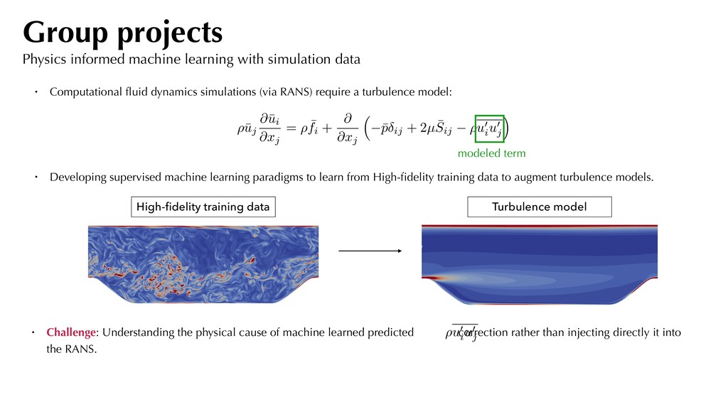
Computational fluid dynamics simulations (via RANS) require a turbulence model: ⇢¯ uj @¯ ui @xj = ⇢ ¯ fi + @ @xj ⇣ ¯ p ij + 2µ ¯ Sij ⇢u0 i u0 j ⌘ modeled term • Challenge: Understanding the physical cause of machine learned predicted correction rather than injecting directly it into the RANS. High-fidelity training data Turbulence model • Developing supervised machine learning paradigms to learn from High-fidelity training data to augment turbulence models. ⇢u0 i u0 j
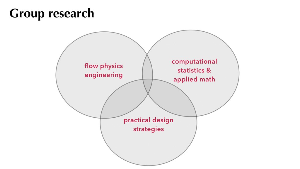
uncertainty quantification, machine learning, optimisation, numerical integration and dimension reduction. • Algorithms and routines build upon extensive collective experience of team members and advisors — with backgrounds ranging from applied statistics, numerical analysis to flow physics engineering. • See: www.effective-quadratures.org
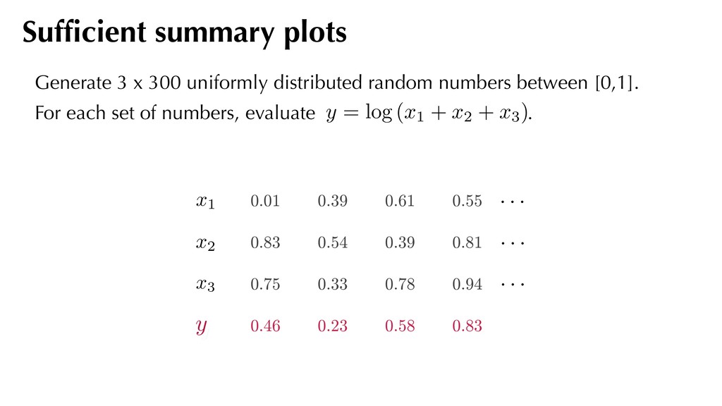
0.78 0.94 0.46 0.23 0.58 0.83 x1 x2 x3 y · · · · · · · · · y Generate 3 x 300 uniformly distributed random numbers between [0,1]. For each set of numbers, evaluate . Sufficient summary plots y = log (x1 + x2 + x3)
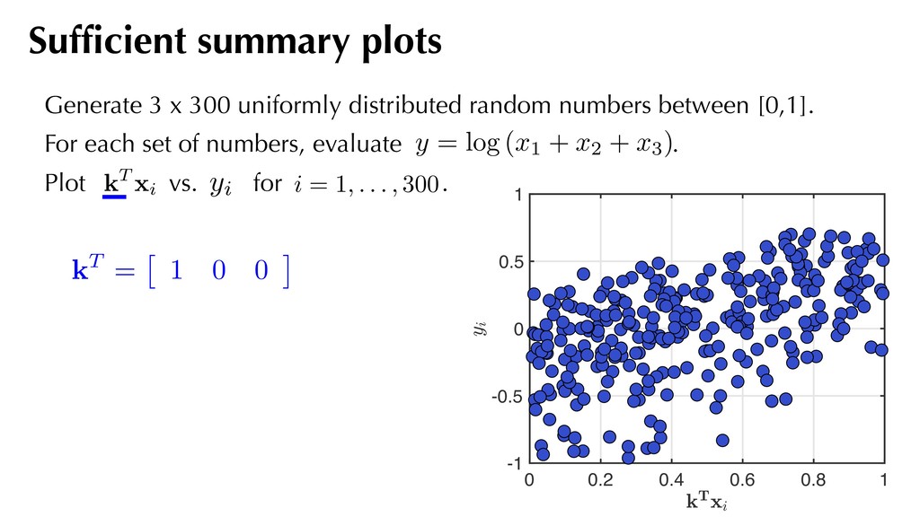
1 kT = ⇥ 1 0 0 ⇤ Generate 3 x 300 uniformly distributed random numbers between [0,1]. For each set of numbers, evaluate . Plot vs. for . Sufficient summary plots kT xi i = 1, . . . , 300 yi y = log (x1 + x2 + x3)
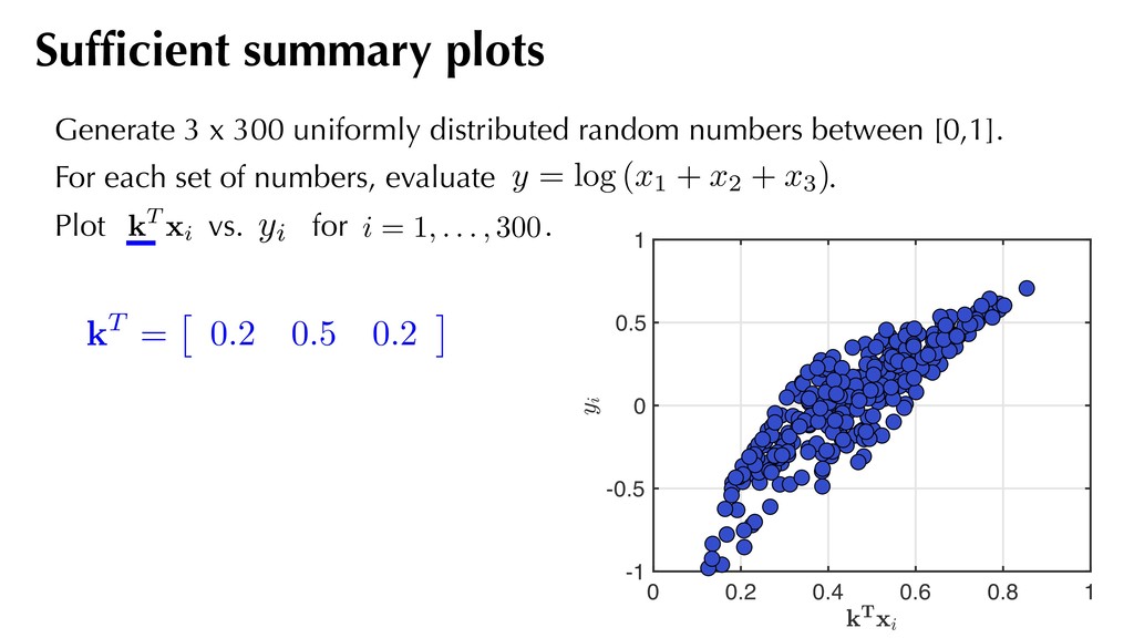
1 kT = ⇥ 0.2 0.5 0.2 ⇤ Generate 3 x 300 uniformly distributed random numbers between [0,1]. For each set of numbers, evaluate . Plot vs. for . Sufficient summary plots kT xi i = 1, . . . , 300 yi y = log (x1 + x2 + x3)
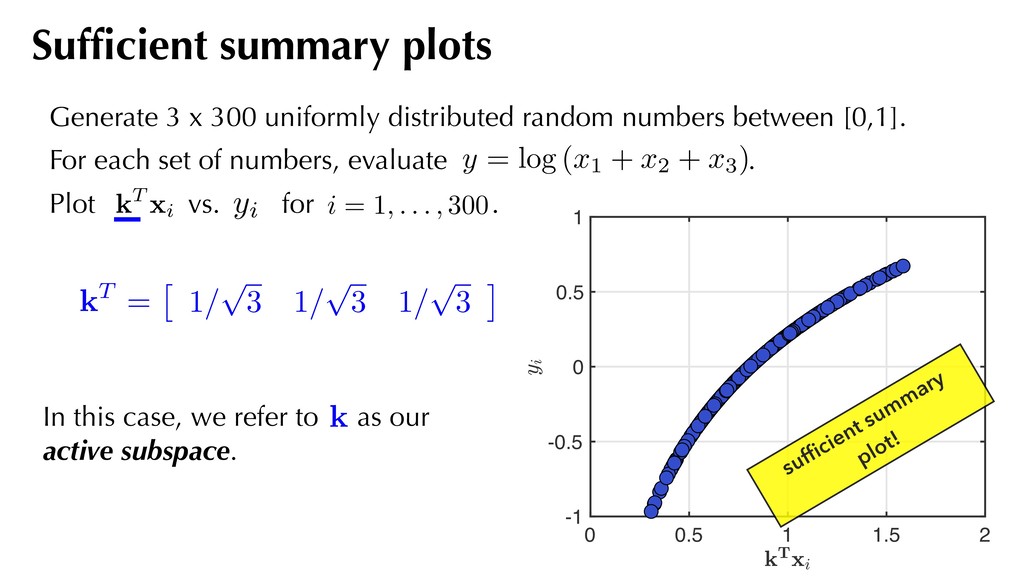
p 3 ⇤ 0 0.5 1 1.5 2 -1 -0.5 0 0.5 1 In this case, we refer to as our active subspace. kT = ⇥ 1/ p 3 1/ p 3 1/ p 3 ⇤ Generate 3 x 300 uniformly distributed random numbers between [0,1]. For each set of numbers, evaluate . Plot vs. for . Sufficient summary plots kT xi i = 1, . . . , 300 yi y = log (x1 + x2 + x3) sufficient summary plot!
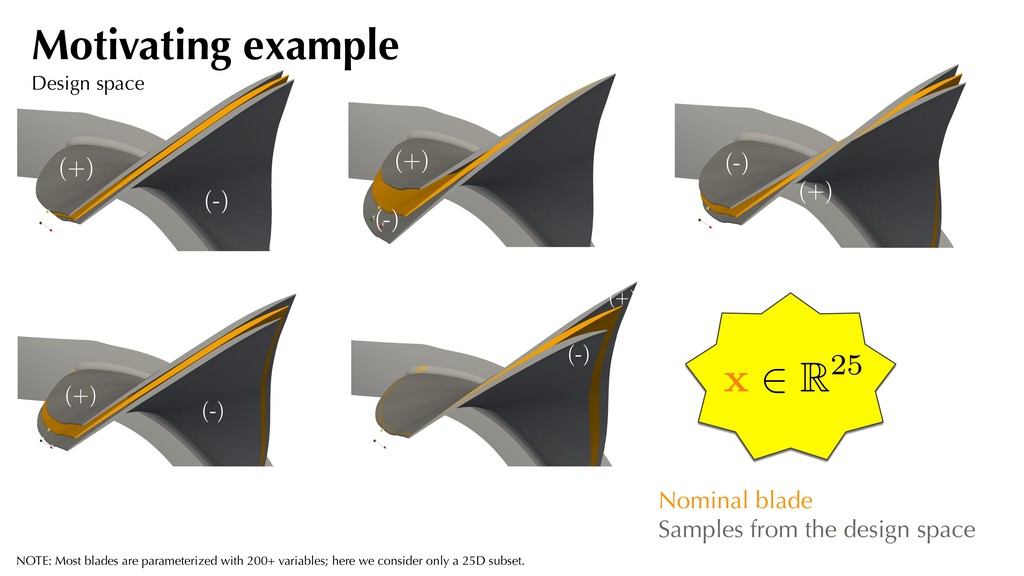
(-) (+) Nominal blade Samples from the design space x 2 R25 NOTE: Most blades are parameterized with 200+ variables; here we consider only a 25D subset. Motivating example Design space
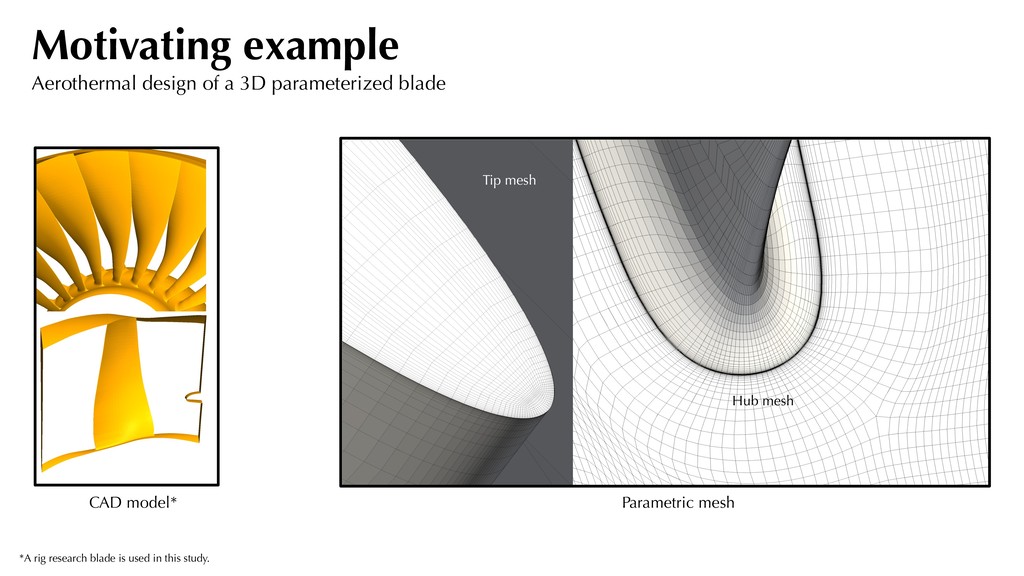
quantities of interest (qoi): geometry mesh PDE solver fj = f (xj) Can study multiple quantities of interest, such as: - Efficiency - Pressure ratio - Flow capacity xj f (xj) We create a data set of N=500 samples. Generate a data-set
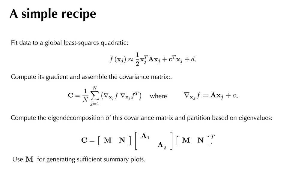
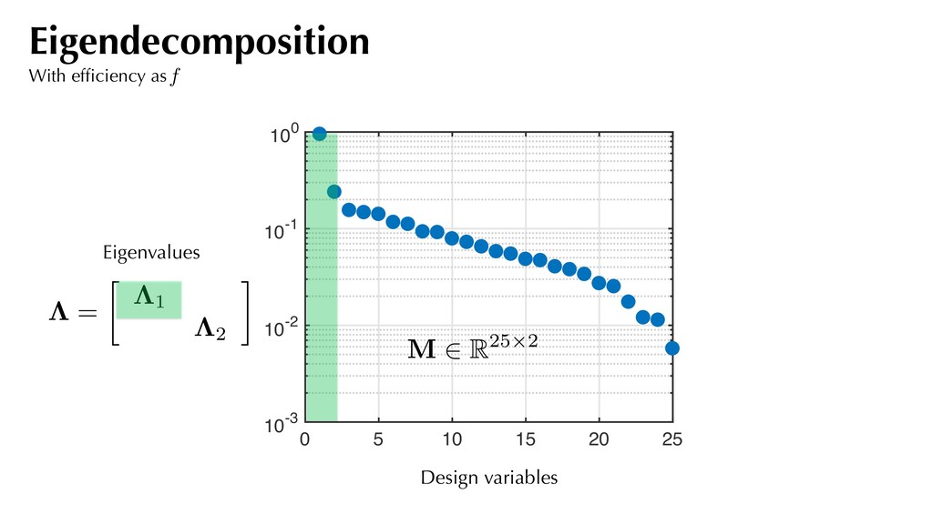
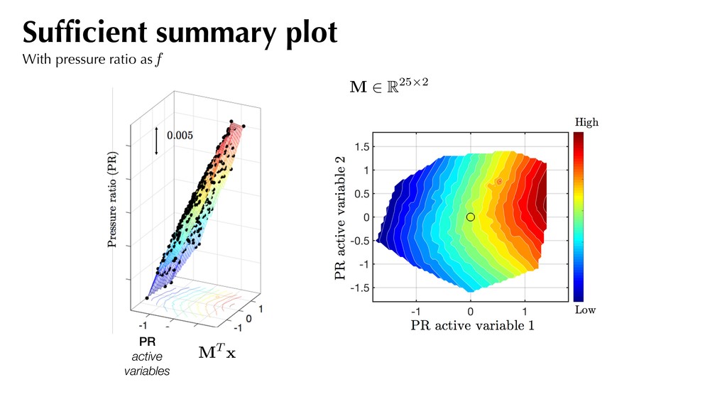
and assemble the covariance matrix:. Compute the eigendecomposition of this covariance matrix and partition based on eigenvalues: f (xj) ⇡ 1 2 xT j Axj + cT xj + d rxj f = Axj + c C = 1 N N X j=1 rxj f rxj fT A simple recipe where C = ⇥ M N ⇤ ⇤1 ⇤1 ⇥ M N ⇤T Use for generating sufficient summary plots. M . . . 2
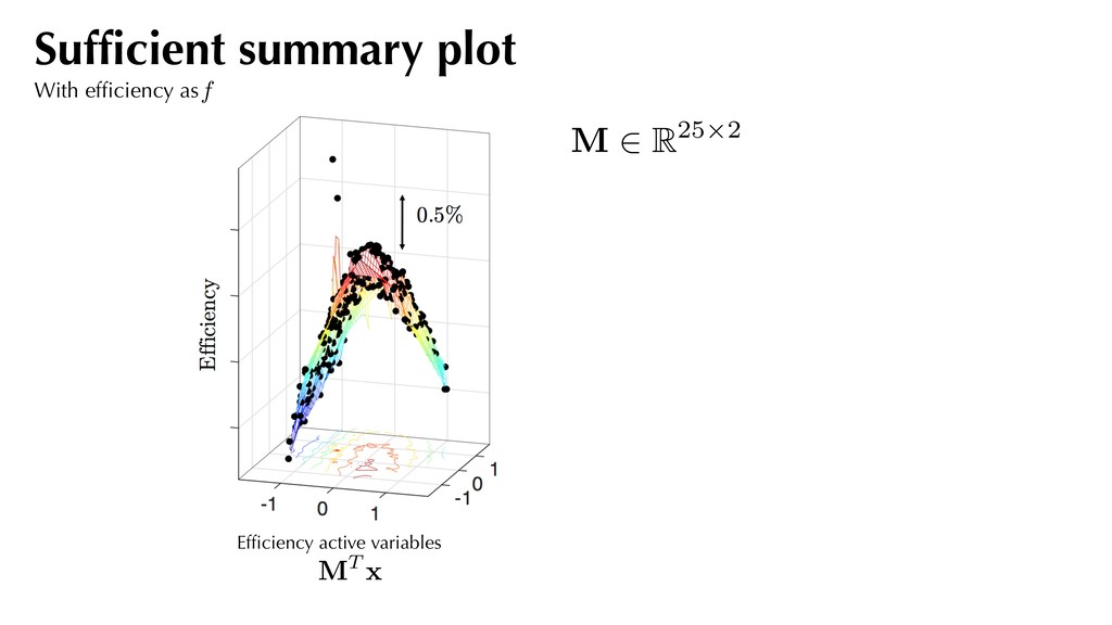
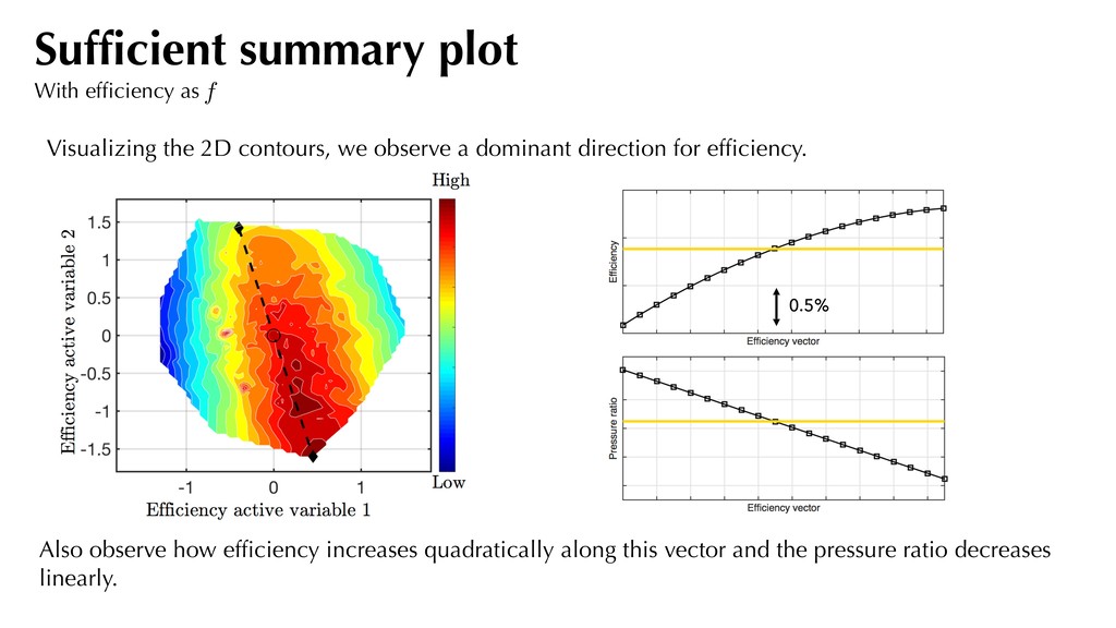
the pressure ratio decreases linearly. Sufficient summary plot With efficiency as f Visualizing the 2D contours, we observe a dominant direction for efficiency. 0.5%
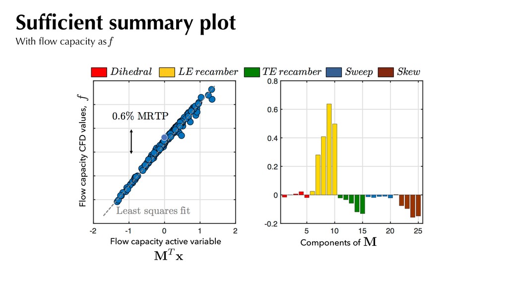
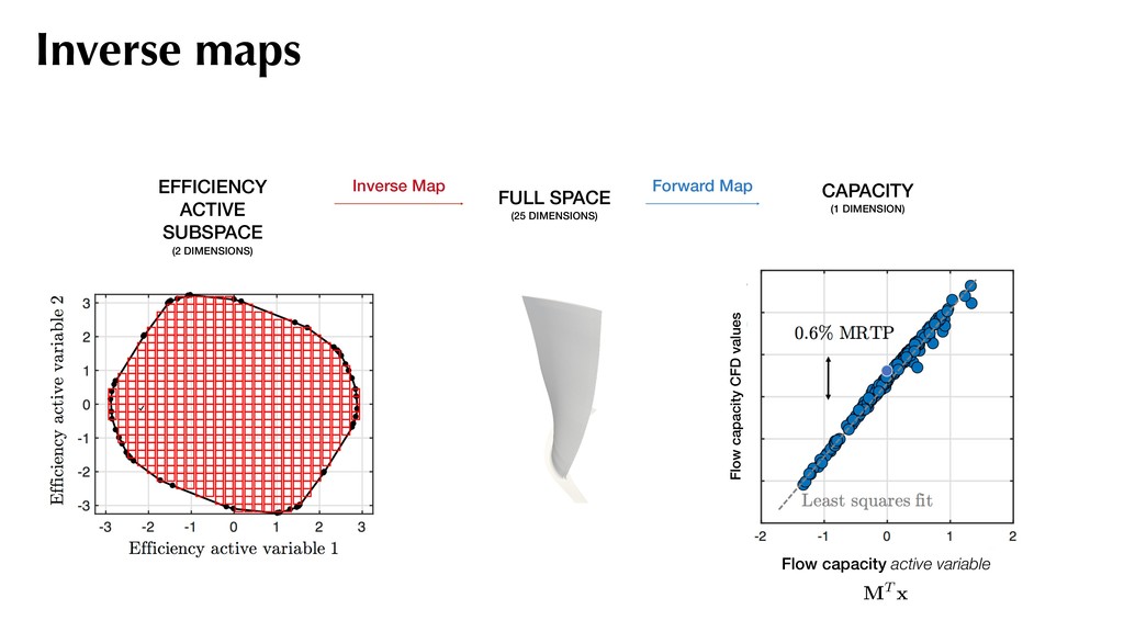
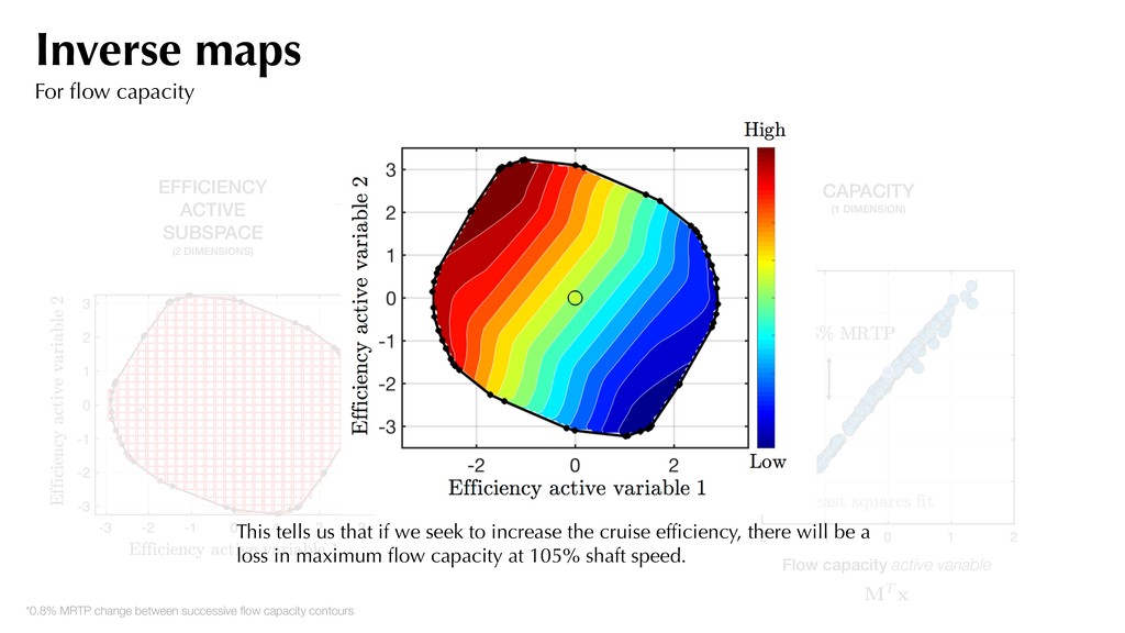
Map Forward Map CAPACITY (1 DIMENSION) Flow capacity active variable Flow capacity CFD values MT x This tells us that if we seek to increase the cruise efficiency, there will be a loss in maximum flow capacity at 105% shaft speed. *0.8% MRTP change between successive flow capacity contours Inverse maps For flow capacity
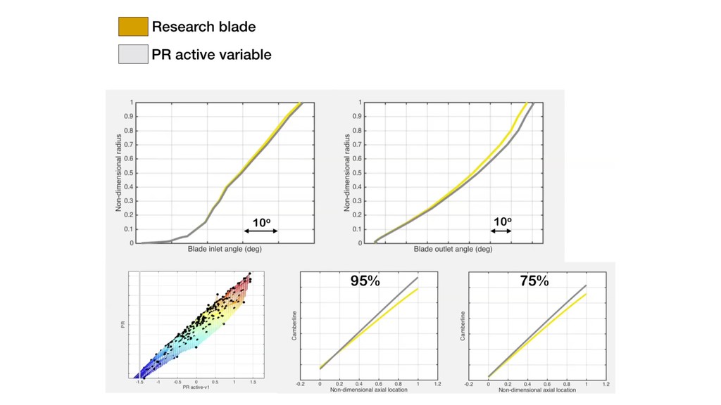
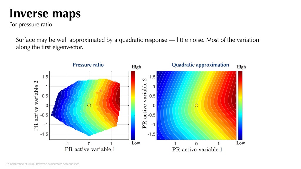
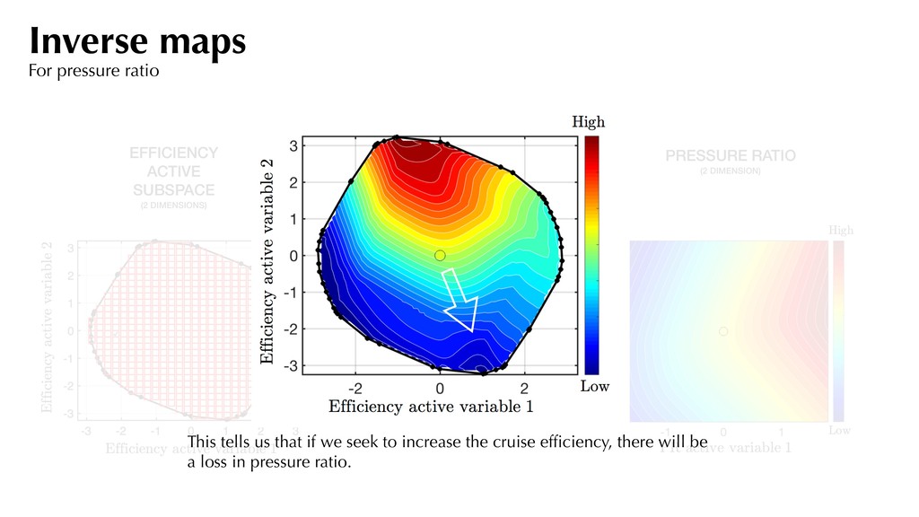
little noise. Most of the variation along the first eigenvector. *PR difference of 0.002 between successive contour lines Pressure ratio Quadratic approximation Inverse maps For pressure ratio
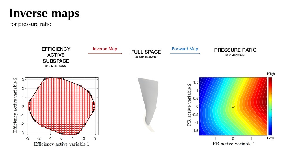
Map Forward Map PRESSURE RATIO (2 DIMENSION) This tells us that if we seek to increase the cruise efficiency, there will be a loss in pressure ratio. Inverse maps For pressure ratio
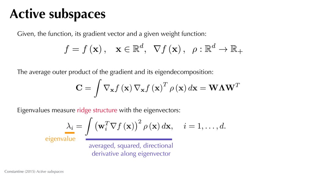
function: f = f (x) , x 2 Rd, rf (x) , ⇢ : Rd ! R + The average outer product of the gradient and its eigendecomposition: Constantine (2015) Active subspaces C = Z rxf (x) rxf (x)T ⇢ (x) dx = W⇤WT Eigenvalues measure ridge structure with the eigenvectors: i = Z wT i rf (x) 2 ⇢ (x) dx, i = 1, . . . , d. eigenvalue averaged, squared, directional derivative along eigenvector Active subspaces
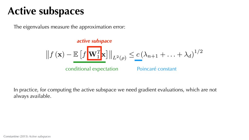
f (x) E ⇥ f|WT 1 x ⇤ L2(⇢) c ( n+1 + . . . + d)1/2 conditional expectation active subspace Poincaré constant In practice, for computing the active subspace we need gradient evaluations, which are not always available. Active subspaces
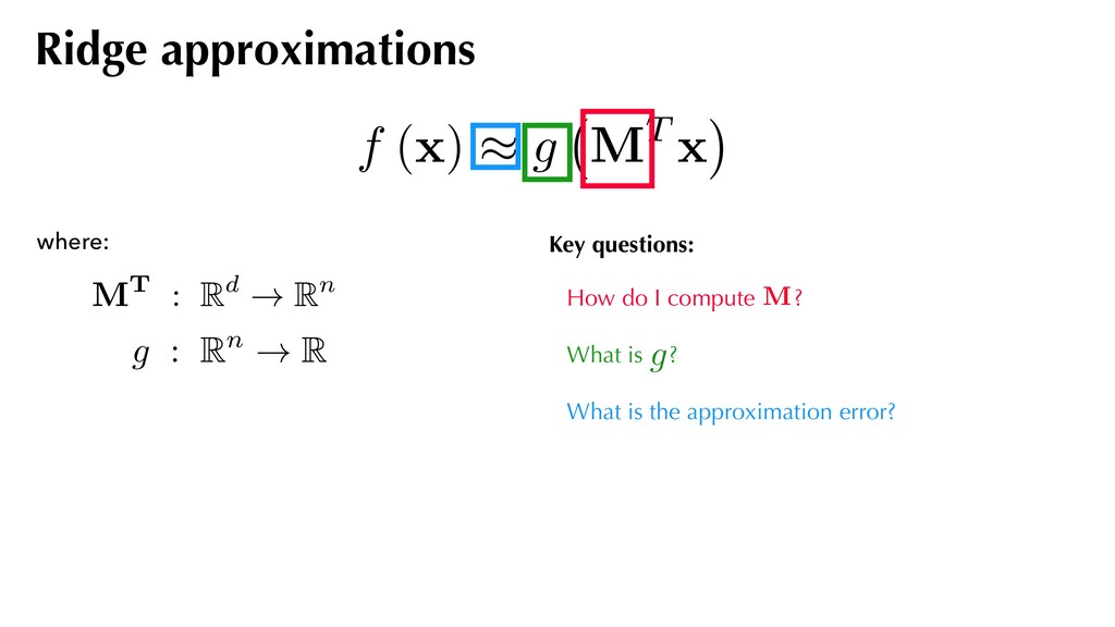
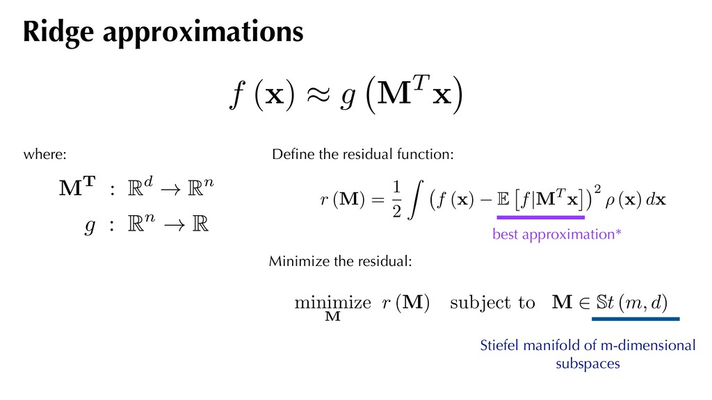
! Rn g : Rn ! R Define the residual function: r (M) = 1 2 Z f (x) E ⇥ f|MT x ⇤ 2 ⇢ (x) dx Minimize the residual: best approximation* minimize M r (M) subject to M 2 St (m, d) Stiefel manifold of m-dimensional subspaces Ridge approximations
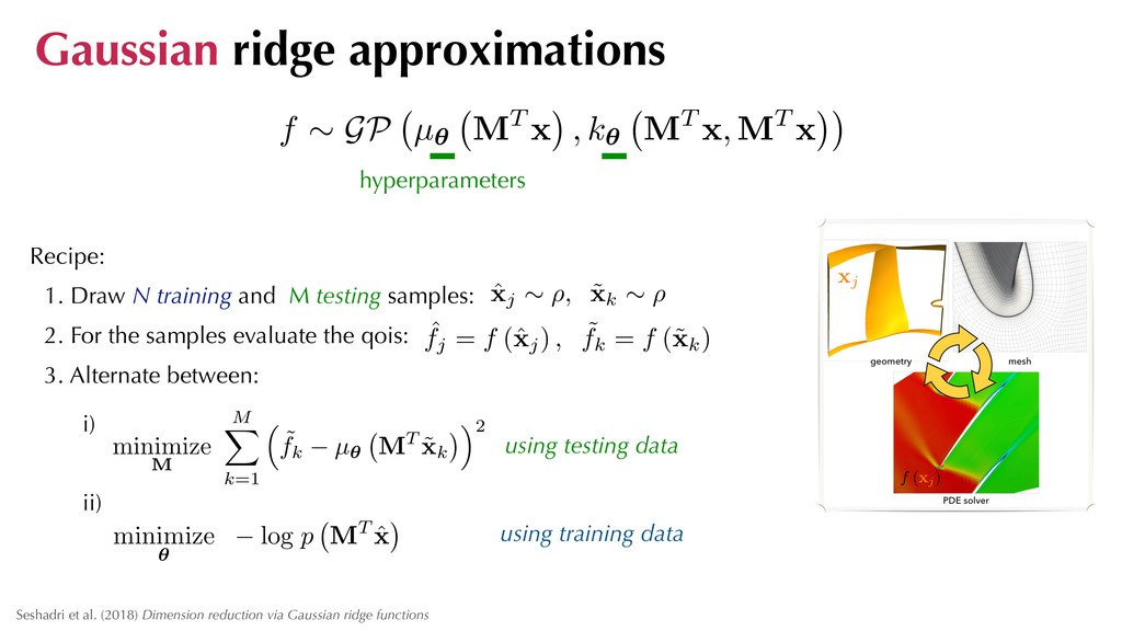
Recipe: 1. Draw N training and M testing samples: 2. For the samples evaluate the qois: 3. Alternate between: i) ii) ˆ fj = f (ˆ xj) , ˜ fk = f (˜ xk) ˆ xj ⇠ ⇢, ˜ xk ⇠ ⇢ f ⇠ GP µ✓ MT x , k✓ MT x, MT x minimize ✓ log p MT ˆ x minimize M M X k=1 ⇣ ˜ fk µ✓ MT ˜ xk ⌘2 using testing data using training data hyperparameters Gaussian ridge approximations
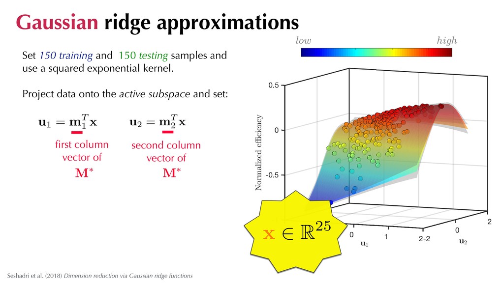
Set 150 training and 150 testing samples and use a squared exponential kernel. Project data onto the active subspace and set: u1 = mT 1 x u2 = mT 2 x first column vector of second column vector of M⇤ M⇤ 5 2 0 0 -5 -2 high low Gaussian ridge approximations x 2 R25
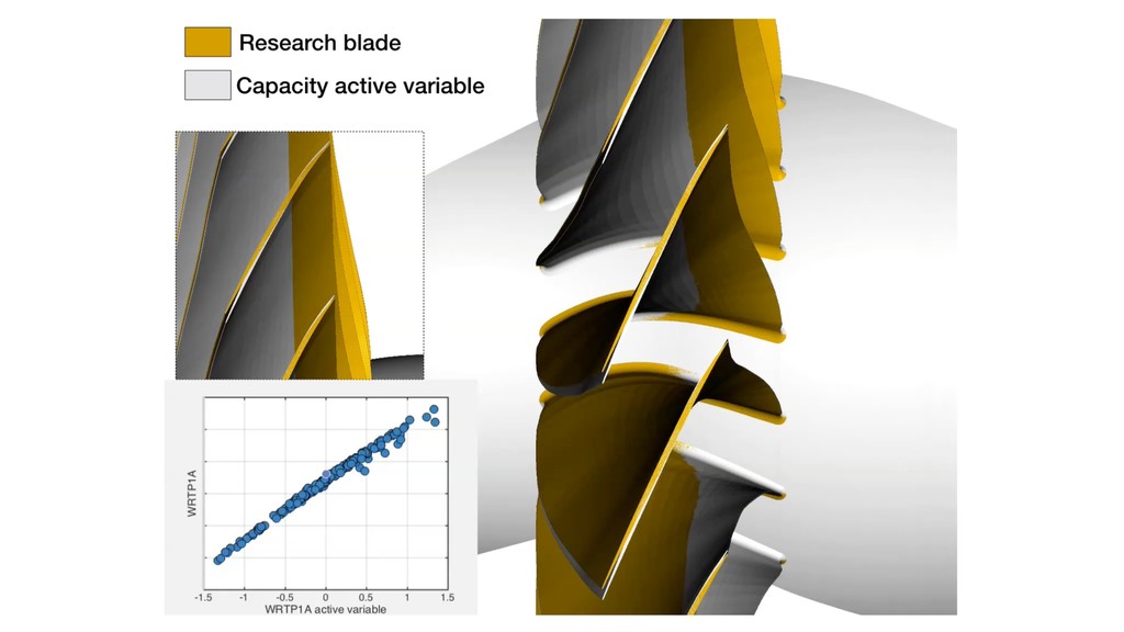
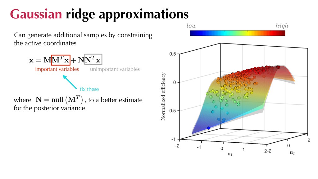
variables where , to a better estimate for the posterior variance. fix these 5 2 0 0 -5 -2 high low Can generate additional samples by constraining the active coordinates Gaussian ridge approximations N = null MT
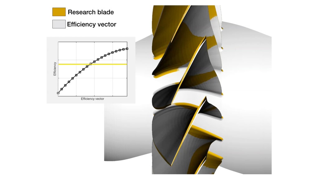
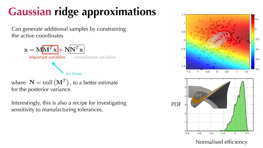
variables where , to a better estimate for the posterior variance. Interestingly, this is also a recipe for investigating sensitivity to manufacturing tolerances. fix these Can generate additional samples by constraining the active coordinates Gaussian ridge approximations N = null MT Normalised efficiency (-) (+) PDF
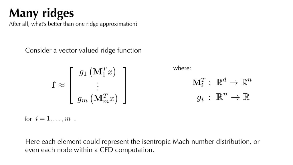
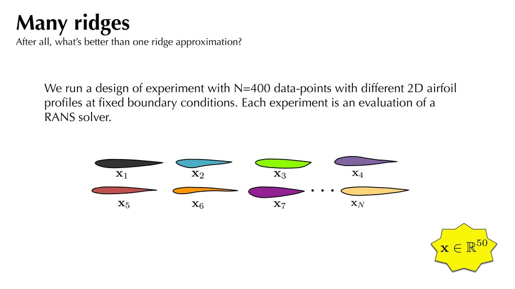
far, we do not really leverage the rich spatial information that CFD affords us. Our interest lies solely with certain output quantities of interest. But are we missing something? Many ridges After all, what’s better than one ridge approximation?
better than one ridge approximation? Here each element could represent the isentropic Mach number distribution, or even each node within a CFD computation. where: MT : Rd ! Rn g : Rn ! R MT i gi f ⇡ 2 6 4 g1 MT 1 x . . . gm MT m x 3 7 5 for . i = 1, . . . , m
different 2D airfoil profiles at fixed boundary conditions. Each experiment is an evaluation of a RANS solver. Many ridges After all, what’s better than one ridge approximation? . . . x1 x2 x3 x4 x5 x6 x7 xN x 2 R50
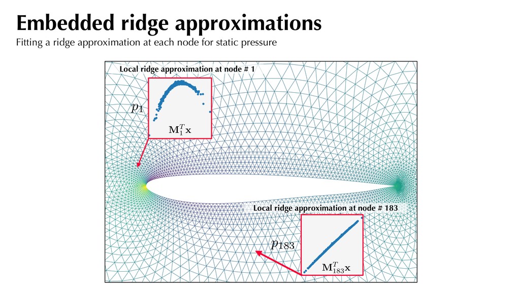
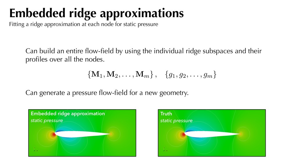
subspaces and their profiles over all the nodes. Can generate a pressure flow-field for a new geometry. Embedded ridge approximation static pressure Truth static pressure Embedded ridge approximations Fitting a ridge approximation at each node for static pressure {M1, M2, . . . , Mm } , {g1, g2, . . . , gm }
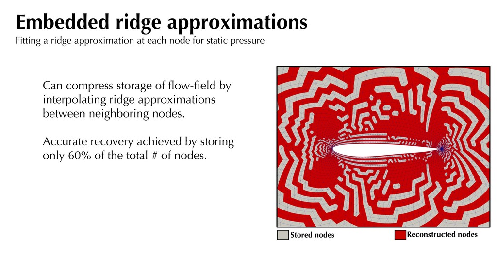
neighboring nodes. Accurate recovery achieved by storing only 60% of the total # of nodes. Embedded ridge approximations Fitting a ridge approximation at each node for static pressure Stored nodes Reconstructed nodes
informs us which parameters are relevant. 2. While many ideas and algorithms exist in literature, there is a need for more — e.g., discrete parameters, strings, multiple subspaces. 3. Working closely with industry, academics need to “lift” these methods to real design problems. Developed workflows must be theoretically sound. 4. Interpretation remains a challenge! Subspaces need not conform to well-understood engineering parameterization.
Scalar-valued dimension reduction Seshadri, Yuchi, Parks. (2020) “Dimension reduction via Gaussian ridge functions”, [accepted] SIAM/ ASA J. on Uncertainty Quantification (special section on approaches to reduce the dimension of model parameters). 2. Vector-valued dimension reduction Wong, Seshadri, Parks, Girolami. (2019) “Embedded ridge approximations: Constructing ridge approximations over scalar fields for improved simulation-centric dimension reduction”, [under review] SIAM/ASA J. on Uncertainty Quantification.
Turing Institute www.psesh.com Research funded by Lloyds Register Foundation Programme for Data-Centric Engineering and UKRI Strategic Priorities Fund under EPSRC Grant P/T001569/1 and Rolls-Royce plc.
![Generate 3 x 300 uniformly distributed random numbers between [0,1].](https://files.speakerdeck.com/presentations/c12237c5fce74042a0822223fc7d3f90/slide_14.jpg)
![xj ⇠ ⇢ Draw samples: From the simulation compute [multiple]](https://files.speakerdeck.com/presentations/c12237c5fce74042a0822223fc7d3f90/slide_24.jpg)