chaos tools that go from a user-defined problem to computing statistics. This may include running relevant computational physics modules*. ▶ Some codes have adaptive capabilities to ensure that statistics provided are suitably converged. ▶ In the context of design, such codes and workflows are useful to assess performance of components under uncertainty. *For those that don’t, recommend www.effective-quadratures.org 2
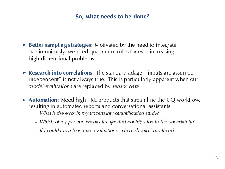
Motivated by the need to integrate parsimoniously, we need quadrature rules for ever increasing high-dimensional problems. ▶ Research into correlations: The standard adage, “inputs are assumed independent” is not always true. This is particularly apparent when our model evaluations are replaced by sensor data. ▶ Automation: Need high TRL products that streamline the UQ workflow, resulting in automated reports and conversational assistants. – What is the error in my uncertainty quantification study? – Which of my parameters has the greatest contribution to the uncertainty? – If I could run a few more evaluations, where should I run them? 3
in this presentation can be found online: https://github.com/Effective-Quadratures/VKI-Talk ▶ You need Python 2.7 and Effective Quadratures to run the codes. 4
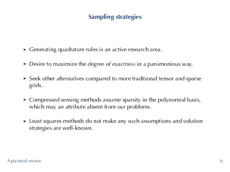
area. ▶ Desire to maximize the degree of exactness in a parsimonious way. ▶ Seek other alternatives compared to more traditional tensor and sparse grids. ▶ Compressed sensing methods assume sparsity in the polynomial basis, which may an attribute absent from our problems. ▶ Least squares methods do not make any such assumptions and solution strategies are well-known. A pictorial review 6
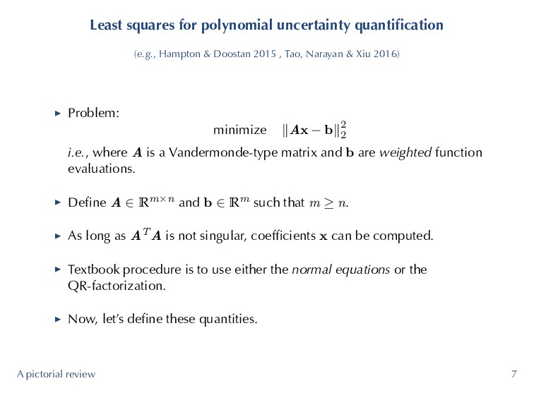
2015 , Tao, Narayan & Xiu 2016) ▶ Problem: minimize ∥Ax − b∥2 2 i.e., where A is a Vandermonde-type matrix and b are weighted function evaluations. ▶ Define A ∈ Rm×n and b ∈ Rm such that m ≥ n. ▶ As long as ATA is not singular, coefficients x can be computed. ▶ Textbook procedure is to use either the normal equations or the QR-factorization. ▶ Now, let’s define these quantities. A pictorial review 7
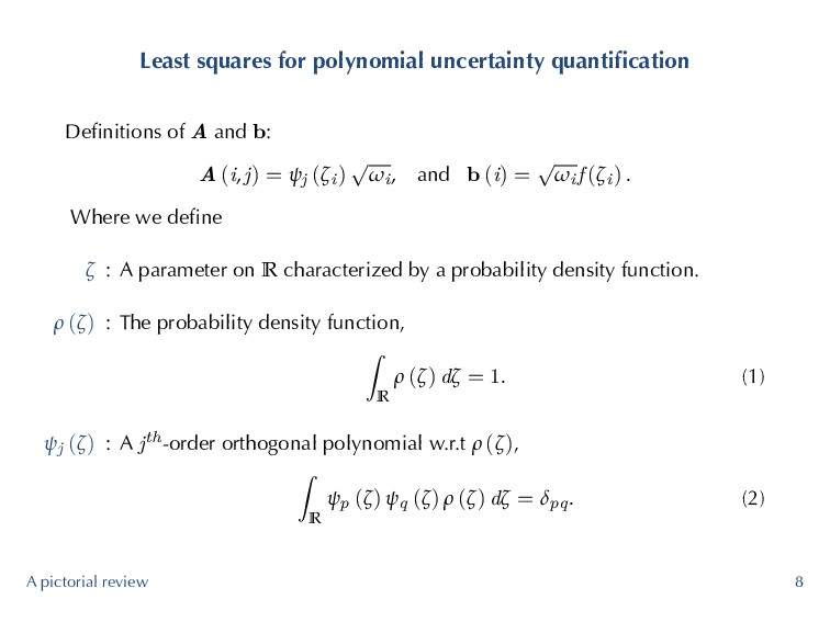
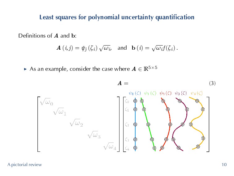
b: A (i, j) = ψj (ζi) √ ωi, and b (i) = √ ωif (ζi) . Where we define ζ : A parameter on R characterized by a probability density function. ρ (ζ) : The probability density function, ˆ R ρ (ζ) dζ = 1. (1) ψj (ζ) : A jth-order orthogonal polynomial w.r.t ρ (ζ), ˆ R ψp (ζ) ψq (ζ) ρ (ζ) dζ = δpq. (2) A pictorial review 8
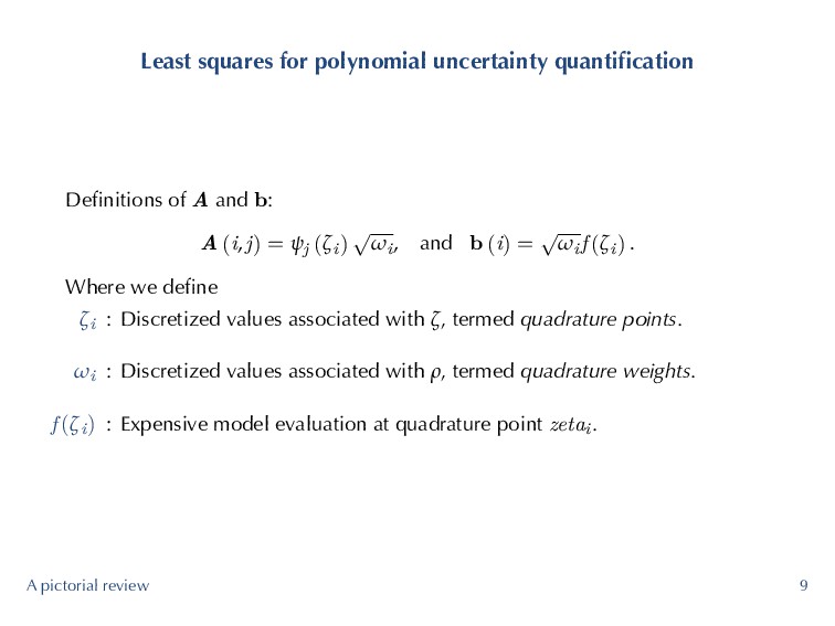
b: A (i, j) = ψj (ζi) √ ωi, and b (i) = √ ωif (ζi) . Where we define ζi : Discretized values associated with ζ, termed quadrature points. ωi : Discretized values associated with ρ, termed quadrature weights. f (ζi) : Expensive model evaluation at quadrature point zetai . A pictorial review 9
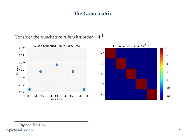
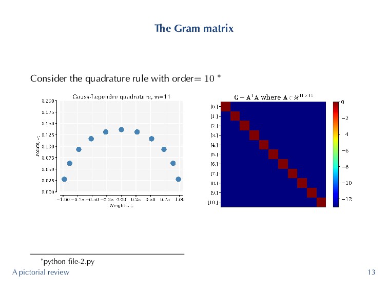
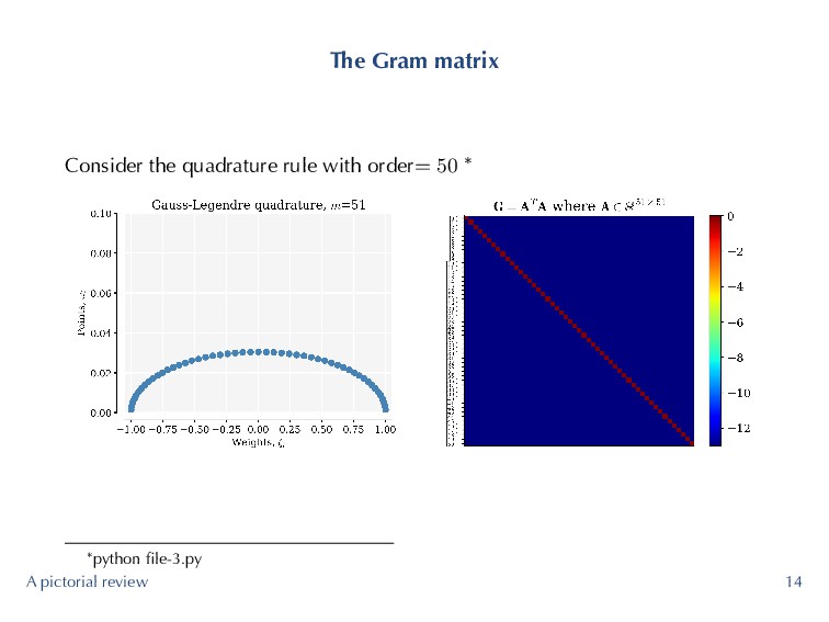
problem further, it will be useful to study the Gram matrix G := ATA. (4) ▶ Each element of the Gram matrix is given by G (p, q) = m−1 ∑ i=0 ψp (ζi) ψq (ζi) ωi ≈ δpq (5) A pictorial review 11
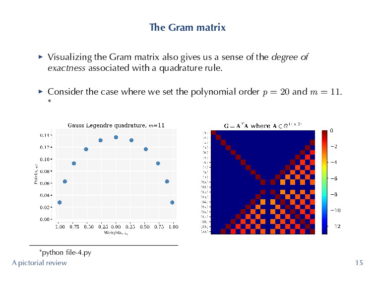
us a sense of the degree of exactness associated with a quadrature rule. ▶ Consider the case where we set the polynomial order p = 20 and m = 11. * *python file-4.py A pictorial review 15
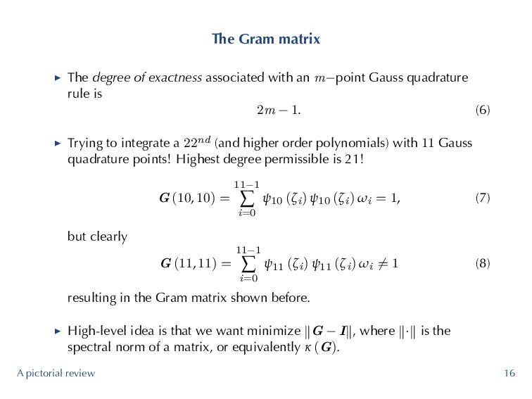
an m−point Gauss quadrature rule is 2m − 1. (6) ▶ Trying to integrate a 22nd (and higher order polynomials) with 11 Gauss quadrature points! Highest degree permissible is 21! G (10, 10) = 11−1 ∑ i=0 ψ10 (ζi) ψ10 (ζi) ωi = 1, (7) but clearly G (11, 11) = 11−1 ∑ i=0 ψ11 (ζi) ψ11 (ζi) ωi ̸= 1 (8) resulting in the Gram matrix shown before. ▶ High-level idea is that we want minimize ∥G − I∥, where ∥·∥ is the spectral norm of a matrix, or equivalently κ (G). A pictorial review 16
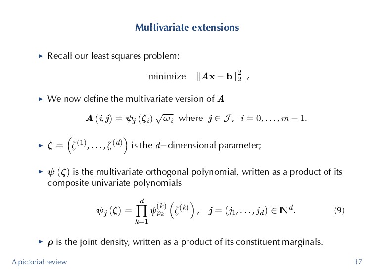
− b∥2 2 , ▶ We now define the multivariate version of A A (i, j) = ψj (ζi) √ ωi where j ∈ J , i = 0, . . . , m − 1. ▶ ζ = ( ζ(1), . . . , ζ(d) ) is the d−dimensional parameter; ▶ ψ (ζ) is the multivariate orthogonal polynomial, written as a product of its composite univariate polynomials ψj (ζ) = d ∏ k=1 ψ(k) pk ( ζ(k) ) , j = (j1, . . . , jd) ∈ Nd. (9) ▶ ρ is the joint density, written as a product of its constituent marginals. A pictorial review 17
& Griebel 2003) ▶ Multivariate extensions of univariate rules exist in the form of tensor product grids, at the cost of md function evaluations. ˆ Rd f (ζ) ρ (ζ) dζ ≈ ( Qm1 q ⊗ . . . ⊗ Qmd q ) (f) = m1 ∑ j1=1 . . . md ∑ jd=1 f (ζjd , . . . , ζjd ) ωj1 . . . ωjd = m ∑ j=1 f (ζj) ωj. (10) ▶ The notation Qmi q denotes a linear operation of the univariate quadrature rule applied to f along direction i; the subscript q stands for quadrature. A pictorial review 19
Gerstner & Griebel 1998) ▶ Sparse grids offer moderate computational attenuation to this problem. One can think of a sparse grid as linear combinations of select anisotropic tensor grids ˆ Rd f (ζ) ρ (ζ) dζ ≈ ∑ r∈K α (r) ( Qm1 q ⊗ . . . ⊗ Qmd q ) (f) . (11) ▶ Here for a given level l—a variable that controls the density of points and the highest order of the polynomial in each direction—the multi-index K and coefficients α(r) are given by K = { r ∈ Nd : l + 1 ≤ |r| ≤ l + d } (12) and α (r) = (−1)−|r|+d+l ( d − 1 − |r| + d + l ) . (13) A pictorial review 20
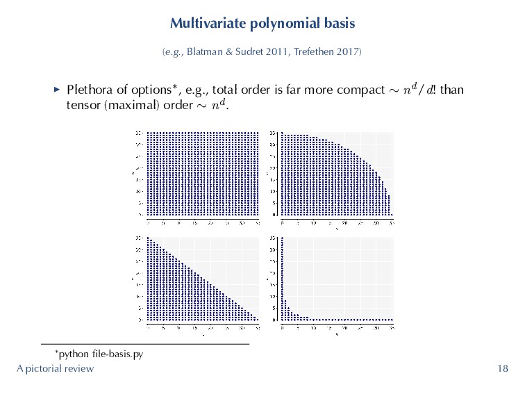
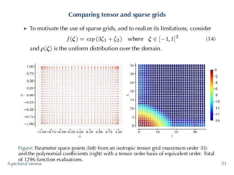
of sparse grids, and to realize its limitations, consider f (ζ) = exp (3ζ1 + ζ2) where ζ ∈ [−1, 1]2 (14) and ρ(ζ) is the uniform distribution over the domain. Figure: Parameter space points (left) from an isotropic tensor grid (maximum order 35) and the polynomial coefficients (right) with a tensor order basis of equivalent order. Total of 1296 function evaluations. A pictorial review 21
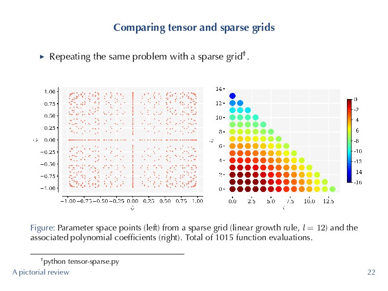
with a sparse grid†. Figure: Parameter space points (left) from a sparse grid (linear growth rule, l = 12) and the associated polynomial coefficients (right). Total of 1015 function evaluations. †python tensor-sparse.py A pictorial review 22
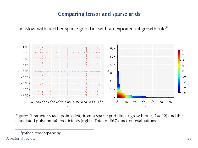
grid, but with an exponential growth rule‡. Figure: Parameter space points (left) from a sparse grid (linear growth rule, l = 12) and the associated polynomial coefficients (right). Total of 667 function evaluations. ‡python tensor-sparse.py A pictorial review 23
note that using tensor or sparse grid quadrature rules§ within least squares yields the exact same coefficients than if one uses pseudospectral projections, i.e., x = ( ATA )−1 ATb = ATb. (15) ▶ Assuming A and b are known, solving this is trivial! ▶ However, the true challenge lies in selecting multivariate quadrature points and weights {(ζi, ωi)}m−1 i=0 , such that m is as close to n as possible. ▶ We will explore different strategies for generating A and techniques for subsampling it. §Care must be taken when using sparse grids, for details see Constantine et al. 2012, CMAME. A pictorial review 24
polynomial least squares is to generate random Monte-Carlo samples based on joint density ρ (ζ) in Rd. ▶ Practical sampling heuristic for well conditioned matrices is m ≥ n2 on total order and hyperbolic cross spaces ¶. ▶ But surely better strategies must exist? We break our problem into two sub-problems 1. Selecting a set of samples 2. Subselecting samples via optimization ¶See Migliorati, Nobile, Schwerin, Tempone, 2014. FCM New quadrature strategies 26
samples significantly outperform standard Monte Carlo (in general). Define the diagonal of the orthogonal projection kernel Kn (ζ) := n ∑ j=1 ψ2 j (ζ) , (16) where subscript n denotes card (J ). ▶ If the domain is bounded with a continuous ρ, then we know that lim n→∞ m Kn (ζ) = ρ (ζ) ν (ζ) , (17) where ν (ζ) is the weighted pluripotential equilibrium measure. ▶ This boils down to sampling from ν (ζ) and modifying the weight function by a constant. New quadrature strategies 27
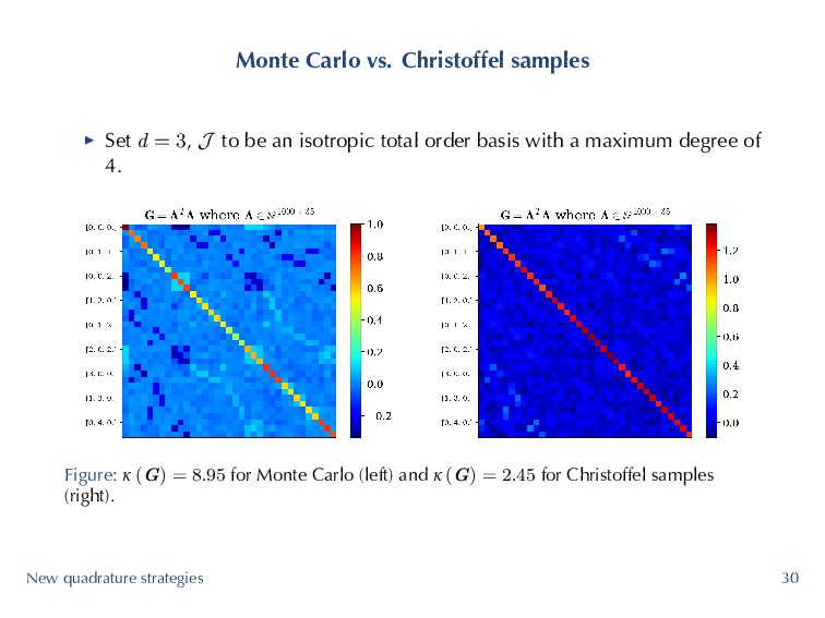
J to be an isotropic total order basis with a maximum degree of 4. Figure: κ (G) = 8.95 for Monte Carlo (left) and κ (G) = 2.45 for Christoffel samples (right). New quadrature strategies 30
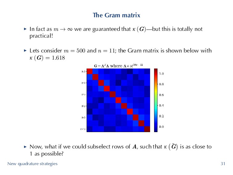
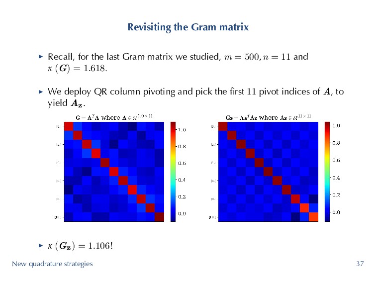
we are guaranteed that κ (G)—but this is totally not practical! ▶ Lets consider m = 500 and n = 11; the Gram matrix is shown below with κ (G) = 1.618 ▶ Now, what if we could subselect rows of A, such that κ ( ˜ G ) is as close to 1 as possible? New quadrature strategies 31
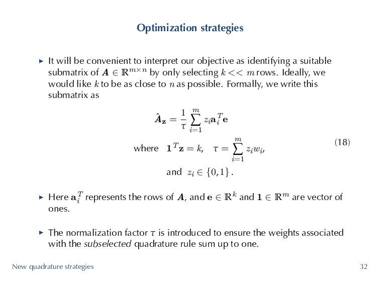
objective as identifying a suitable submatrix of A ∈ Rm×n by only selecting k << m rows. Ideally, we would like k to be as close to n as possible. Formally, we write this submatrix as ˆ Az = 1 τ m ∑ i=1 ziaT i e where 1Tz = k, τ = m ∑ i=1 ziwi, and zi ∈ {0, 1} . (18) ▶ Here aT i represents the rows of A, and e ∈ Rk and 1 ∈ Rm are vector of ones. ▶ The normalization factor τ is introduced to ensure the weights associated with the subselected quadrature rule sum up to one. New quadrature strategies 32
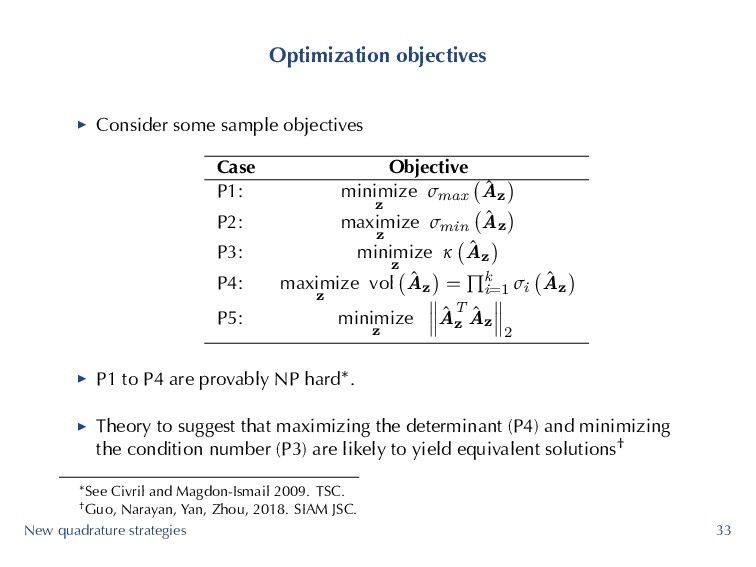
minimize z σmax ( ˆ Az ) P2: maximize z σmin ( ˆ Az ) P3: minimize z κ ( ˆ Az ) P4: maximize z vol ( ˆ Az ) = ∏k i=1 σi ( ˆ Az ) P5: minimize z ˆ AT z ˆ Az 2 ▶ P1 to P4 are provably NP hard*. ▶ Theory to suggest that maximizing the determinant (P4) and minimizing the condition number (P3) are likely to yield equivalent solutions† *See Civril and Magdon-Ismail 2009. TSC. †Guo, Narayan, Yan, Zhou, 2018. SIAM JSC. New quadrature strategies 33
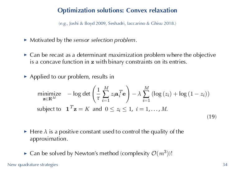
Iaccarino & Ghisu 2018.) ▶ Motivated by the sensor selection problem. ▶ Can be recast as a determinant maximization problem where the objective is a concave function in z with binary constraints on its entries. ▶ Applied to our problem, results in minimize z∈RM − log det ( 1 τ M ∑ i=1 ziaT i e ) − λ M ∑ i=1 (log (zi) + log (1 − zi)) subject to 1Tz = K and 0 ≤ zi ≤ 1, i = 1, . . . , M. (19) ▶ Here λ is a positive constant used to control the quality of the approximation. ▶ Can be solved by Newton’s method (complexity O(m3))! New quadrature strategies 34
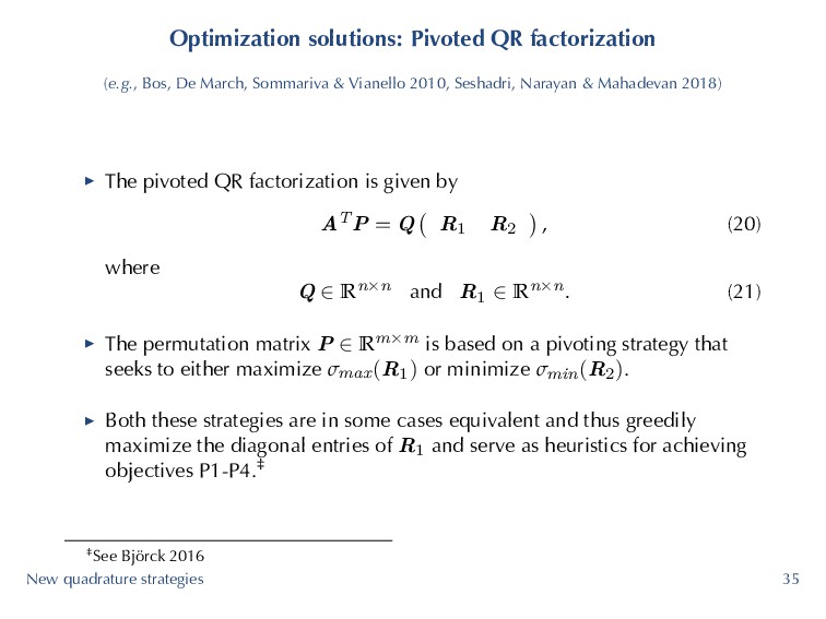
& Vianello 2010, Seshadri, Narayan & Mahadevan 2018) ▶ The pivoted QR factorization is given by ATP = Q ( R1 R2 ) , (20) where Q ∈ Rn×n and R1 ∈ Rn×n. (21) ▶ The permutation matrix P ∈ Rm×m is based on a pivoting strategy that seeks to either maximize σmax(R1) or minimize σmin(R2). ▶ Both these strategies are in some cases equivalent and thus greedily maximize the diagonal entries of R1 and serve as heuristics for achieving objectives P1-P4.‡ ‡See Björck 2016 New quadrature strategies 35
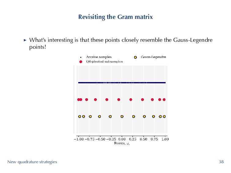
matrix we studied, m = 500, n = 11 and κ (G) = 1.618. ▶ We deploy QR column pivoting and pick the first 11 pivot indices of A, to yield Az . ▶ κ (Gz) = 1.106! New quadrature strategies 37
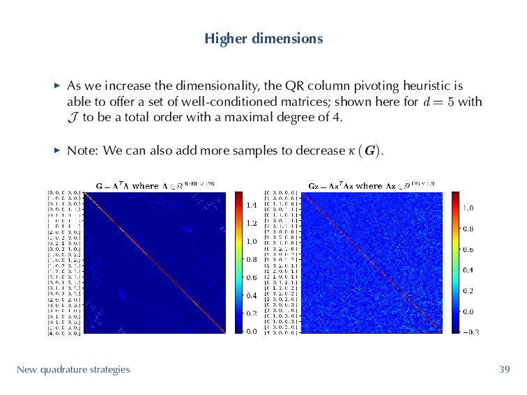
column pivoting heuristic is able to offer a set of well-conditioned matrices; shown here for d = 5 with J to be a total order with a maximal degree of 4. ▶ Note: We can also add more samples to decrease κ (G). New quadrature strategies 39
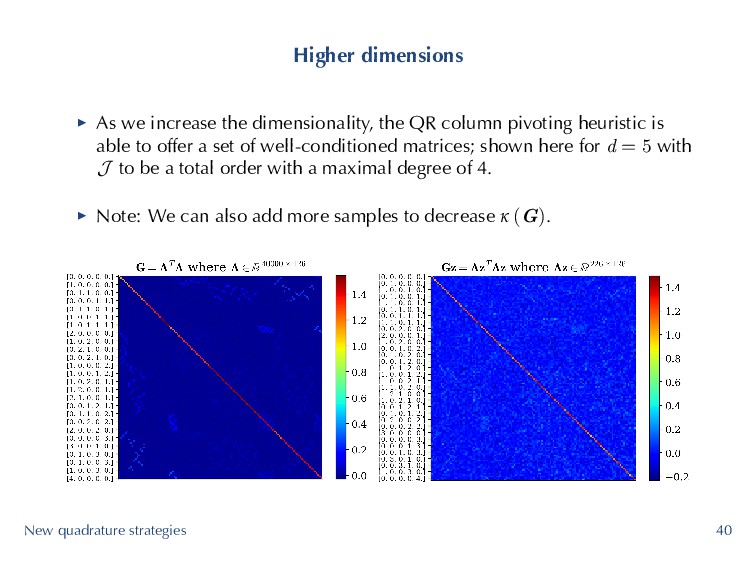
column pivoting heuristic is able to offer a set of well-conditioned matrices; shown here for d = 5 with J to be a total order with a maximal degree of 4. ▶ Note: We can also add more samples to decrease κ (G). New quadrature strategies 40
in generating quadrature rules on total degree and hyperbolic basis—leveraging the anisotropic structure of physical problem. ▶ Interpolation and approximation with even total order basis encounter the pervasive challenges of uniqueness and existence (unisolvency). ▶ Key question: How do we interpolate / approximate with these non-tensorial bases; where should the points be distributed? New quadrature strategies 41
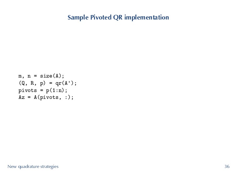
Narayan & Mahadevan 2018) A few recipes: ▶ Randomized quadratures: Randomly select ∝ nlog (n) samples from a tensor grid of the chosen order. Use QR column pivoting to prune down the number of samples to n. ▶ Effectively subsampled quadratures: Apply QR column pivoting to all samples in the tensor product grid and then select the points corresponding to the top n pivots. ▶ Christoffel least squares: Randomly select ∝ nlog (n) samples from the equilibrium measure. Use QR column pivoting to prune down the number of samples to n. New quadrature strategies 42
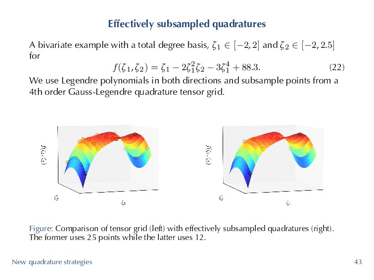
basis, ζ1 ∈ [−2, 2] and ζ2 ∈ [−2, 2.5] for f (ζ1, ζ2) = ζ1 − 2ζ2 1ζ2 − 3ζ4 1 + 88.3. (22) We use Legendre polynomials in both directions and subsample points from a 4th order Gauss-Legendre quadrature tensor grid. Figure: Comparison of tensor grid (left) with effectively subsampled quadratures (right). The former uses 25 points while the latter uses 12. New quadrature strategies 43
minimize ∥Ax − b∥2 2 . ▶ We have so far assumed that b is fixed. ▶ In CFD 2.0, b is no longer a deterministic vector, as each function call will have f (ζi) = fi ± f′ i, (23) variability characterized by an interval or distribution*. ▶ Naively, we can assume that the variation in b ∼ N (µb, Σb) and propagate through. *Owing to epistemic uncertainty work by Iaccarino, Duraisamy, Gorle, Emory and others Getting ready for CFD 2.0 45
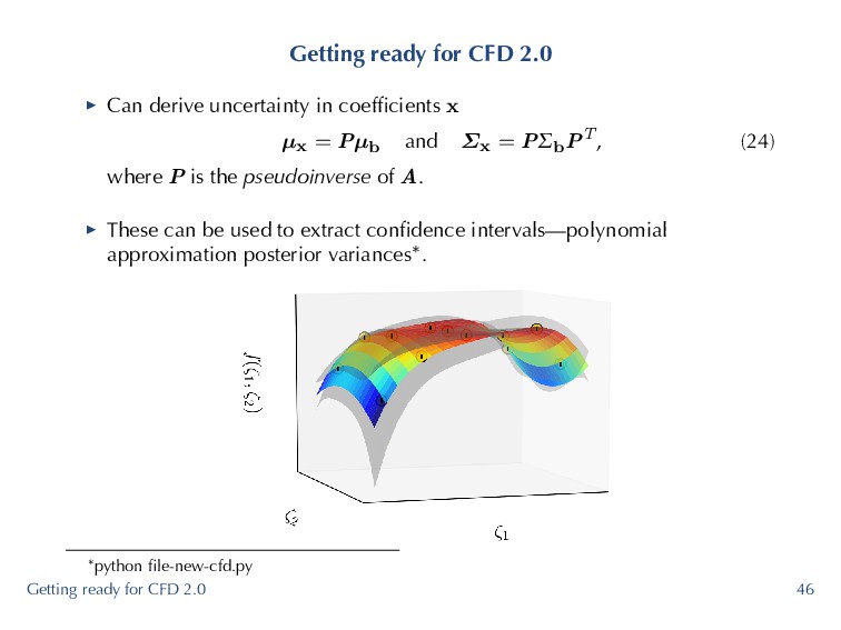
coefficients x µx = Pµb and Σx = PΣbPT, (24) where P is the pseudoinverse of A. ▶ These can be used to extract confidence intervals—polynomial approximation posterior variances*. *python file-new-cfd.py Getting ready for CFD 2.0 46
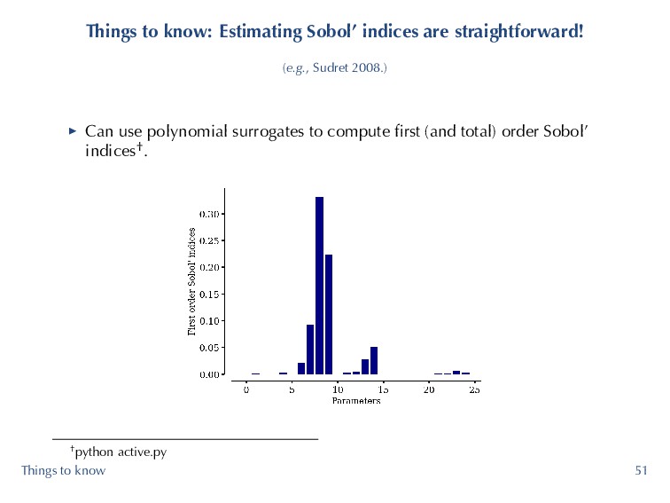
∥Ax − b∥2 2 . ▶ But there are other approaches for estimating x, such as LASSO, basis pursuit, etc. ▶ Regardless of how we compute x, estimating moments are trivial E [f] = x0 and σ2 [f] = n−1 ∑ i=1 x2 i . (25) ▶ So what else can we do? Things to know 48
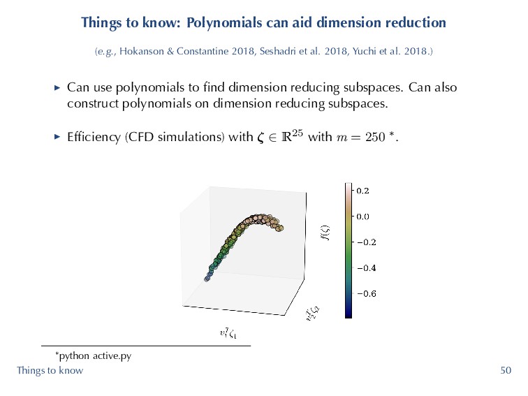
& Constantine 2018, Seshadri et al. 2018, Yuchi et al. 2018.) ▶ Can use polynomials to find dimension reducing subspaces. Can also construct polynomials on dimension reducing subspaces. ▶ Efficiency (CFD simulations) with ζ ∈ R25 with m = 250 *. *python active.py Things to know 50