J. Ball, E. Bayne, P . Belagus, S. Bennett, R. Berger, M. Betts, J. Bielech, A. Bismanis, R. Brown, M. Cadman, D. Collister, M. Cranny, S. Cumming, L. Darling, M. Darveau, C. De La Mare, A. Desrochers, T. Diamond, M. Donnelly, C. Downs, P . Drapeau, C. Duane, B. Dube, D. Dye, R. Eccles, P . Farrington, R. Fernandes, M. Flamme, D. Fortin, K. Foster, M. Gill, T. Gotthardt, N. Guldager, R. Hall, C. Handel, S. Hannon, B. Harrison, C. Harwood, J. Herbers, K. Hobson, M.-A. Hudson, L. Imbeau, P . Johnstone, V. Keenan, K. Koch, M. Laker, S. Lapointe, R. Latifovic, R. Lauzon, M. Leblanc, L. Ledrew, J. Lemaitre, D. Lepage, B. MacCallum, P . MacDonell, C. Machtans, C. McIntyre, M. McGovern, D. McKenney, S. Mason, L. Morgantini, L. Morton, G. Niemi, T. Nudds, P . Papadol, M. Phinney, D. Phoenix, D. Pinaud, D. Player, D. Price, R. Rempel, A. Rosaasen, S. Running, R. Russell, C. Savignac, J. Schieck, F . Schmiegelow, D. Shaw, P . Sinclair, A. Smith, S. Song, C. Spytz, D. Swanson, S. Swanson, P . Taylor, S. Van Wilgenburg, P . Vernier, M.-A. Villard, D. Whitaker, T. Wild, J. Witiw, S. Wyshynski, M. Yaremko, as well as the hundred of volunteers collecting Breeding Bird Survey (BBS) data. Institutions Acadia University; Alaska Bird Observatory; Alaska Natural Heritage Program; Alberta Biodiversity Monitoring Institute; Alberta Pacific Forest Industries Inc.; AMEC Earth & Environmental; AREVA Resources Canada Inc.; Avian Knowledge Network; AXYS Environmental Consulting Ltd.; Bighorn Wildlife Technologies Ltd.; Bird Studies Canada; Breeding Bird Survey (coordinated in Canada by Environment Canada); BC Breeding Bird Atlas; Canadian Natural Resources Ltd.; Canfor Corporation; Daishowa Marubeni International Ltd; Canada Centre for Remote Sensing and Canadian Forest Service, Natural Resources Canada; Canadian Wildlife Service and Science & Technology Branch, Environment Canada; Global Land Cover Facility; Golder Associates Ltd.; Government of British Columbia; Government of Yukon; Hinton Wood Products; Hydro-Québec Équipement; Kluane Ecosystem Monitoring Project; Komex International Ltd.; Louisiana Pacific Canada Ltd.; Manitoba Breeding Bird Atlas; Manitoba Hydro; Manitoba Model Forest Inc.; Manning Diversified Forest Products Ltd.; Maritimes Breeding Bird Atlas; Matrix Solutions Inc. Environment & Engineering; MEG Energy Corp.; Mirkwood Ecological Consultants Ltd.; NatureCounts; Nature Serve; Numerical Terradynamic Simulation Group; Ontario Breeding Bird Atlas; Ontario Ministry of Natural Resources; OPTI Canada Inc.; PanCanadian Petroleum Limited; Parks Canada (Mountain National Parks Avian Monitoring Database); Petro Canada; Principal Wildlife Resource Consulting; Regroupement QuébecOiseaux; Rio Alto Resources International Inc.; Saskatchewan Environment; Shell Canada Ltd.; Suncor Energy Inc.; Tembec Industries Inc.; Tolko Industries Ltd.; U.S. Army; U.S. Fish and Wildlife Service; U.S. Geological Survey, Alaska Science Center; U.S. National Park Service; Université de Moncton; Université du Québec à Montréal; Université du Québec en Abitibi-Témiscamingue; Université Laval; University of Alaska, Fairbanks; University of Alberta; University of British Columbia; University of Guelph; University of New Brunswick; University of Northern British Columbia; URSUS Ecosystem Management Ltd.; West Fraser Timber Co. Ltd.; Weyerhaeuser Company Ltd.; Wildlife Resource Consulting Services MB Inc.
![N PIF E[Y 1 ] P T adj Area 1](https://files.speakerdeck.com/presentations/d1b17a04a32844c0acf169b8429ca328/slide_19.jpg)
![N PIF N PIX E[Y 1 ] E[Y 0 ]](https://files.speakerdeck.com/presentations/d1b17a04a32844c0acf169b8429ca328/slide_20.jpg)
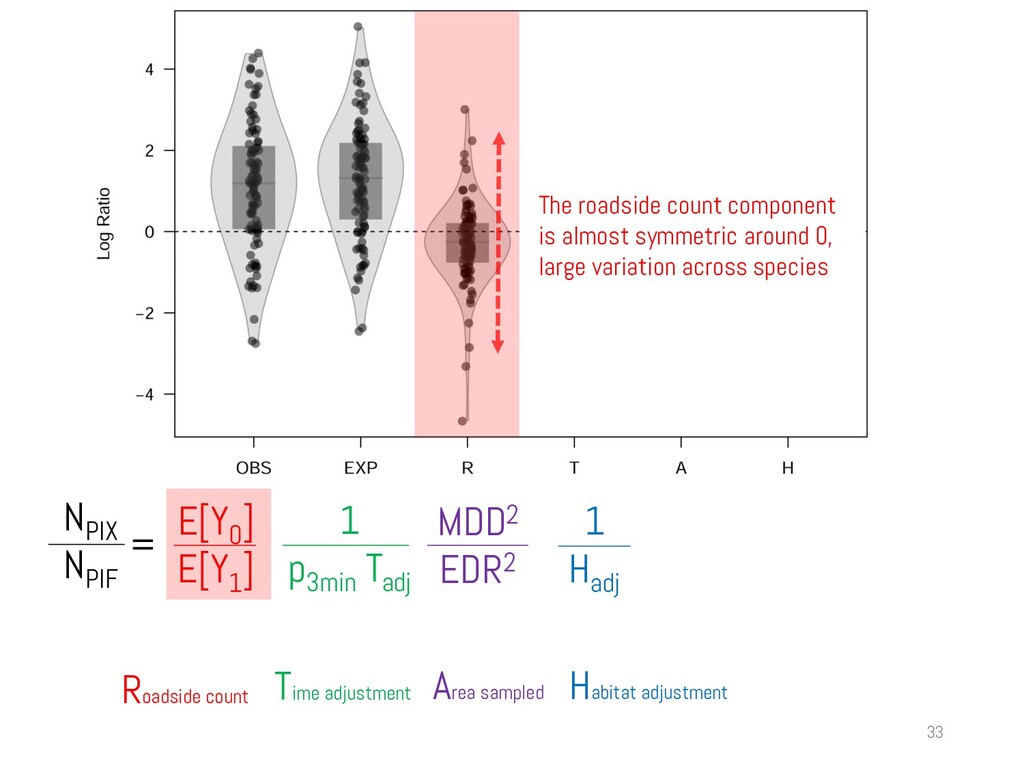
![N PIF N PIX E[Y 1 ] E[Y 0 ]](https://files.speakerdeck.com/presentations/d1b17a04a32844c0acf169b8429ca328/slide_21.jpg)
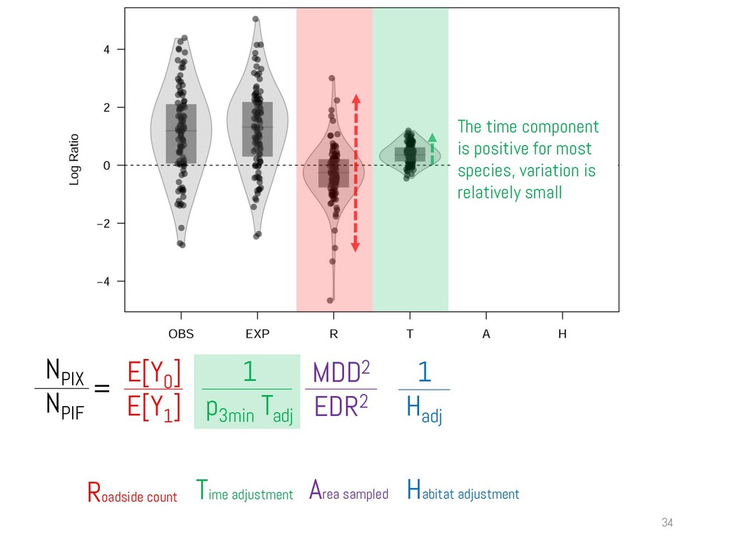
![N PIF N PIX E[Y 1 ] E[Y 0 ]](https://files.speakerdeck.com/presentations/d1b17a04a32844c0acf169b8429ca328/slide_22.jpg)
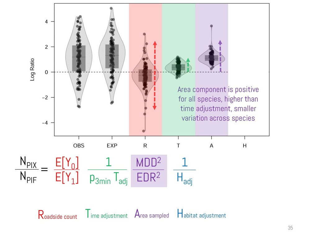
![N PIF N PIX E[Y 1 ] E[Y 0 ]](https://files.speakerdeck.com/presentations/d1b17a04a32844c0acf169b8429ca328/slide_23.jpg)
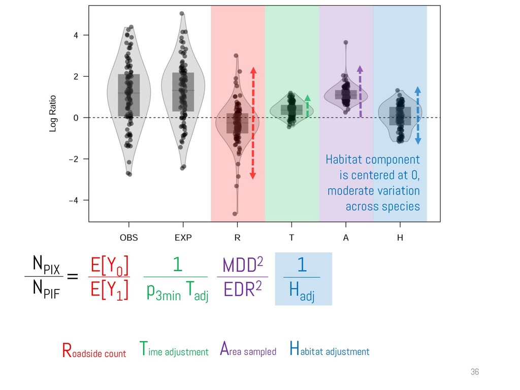
![N PIF N PIX E[Y 1 ] E[Y 0 ]](https://files.speakerdeck.com/presentations/d1b17a04a32844c0acf169b8429ca328/slide_24.jpg)