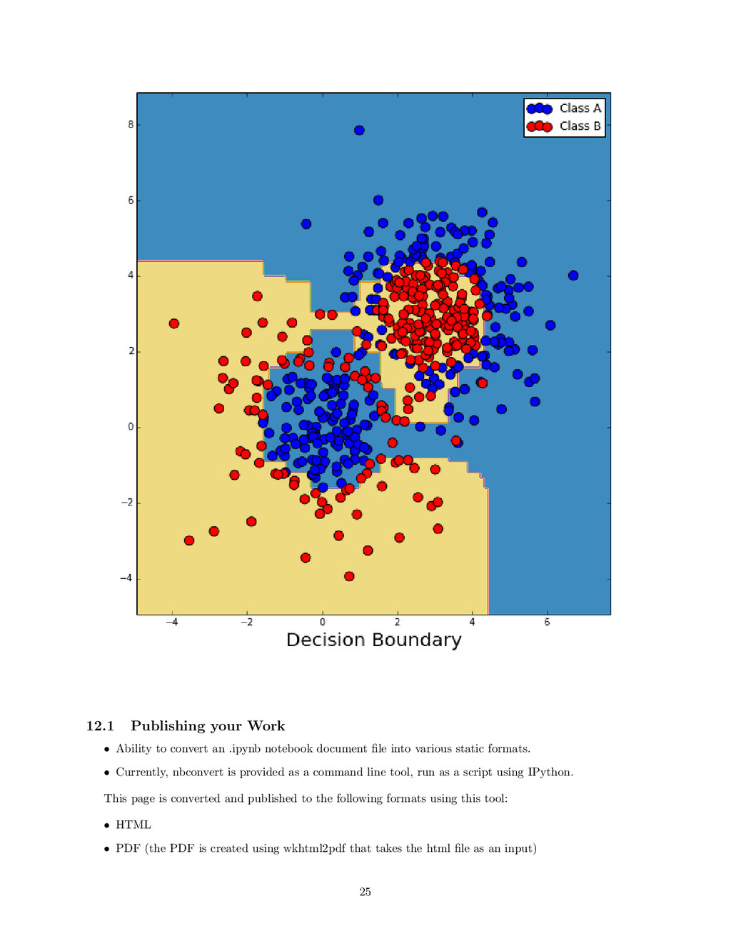
True import pylab as pl import numpy as np from sklearn.ensemble import AdaBoostClassifier from sklearn.tree import DecisionTreeClassifier from sklearn.datasets import make_gaussian_quantiles # Construct dataset X1, y1 = make_gaussian_quantiles(cov=2., n_samples=200, n_features=2, n_classes=2, random_state=1) X2, y2 = make_gaussian_quantiles(mean=(3, 3), cov=1.5, n_samples=300, n_features=2, n_classes=2, random_state=1) #Training Samples X = np.concatenate((X1, X2)) #Training Target y = np.concatenate((y1, - y2 + 1)) # Create and fit an AdaBoosted decision tree bdt = AdaBoostClassifier( DecisionTreeClassifier( max_depth=1), algorithm="SAMME", n_estimators=200 ) bdt.fit(X, y) plot_colors = "br" plot_step = 0.05 class_names = "AB" pl.figure(figsize=(20, 10)) x_min, x_max = X[:, 0].min() - 1, X[:, 0].max() + 1 y_min, y_max = X[:, 1].min() - 1, X[:, 1].max() + 1 if solve: # Plot the decision boundaries pl.subplot(121) xx, yy = np.meshgrid(np.arange(x_min, x_max, plot_step), np.arange(y_min, y_max, plot_step)) Z = bdt.predict(np.c_[xx.ravel(), yy.ravel()]) Z = Z.reshape(xx.shape) cs = pl.contourf(xx, yy, Z, cmap=pl.cm.Paired) 23
![In [8]: #press tab to autocplete long_silly_dummy_name_2 Out[8]: <function main](https://files.speakerdeck.com/presentations/969ec830302c013297b132228b43df58/slide_6.jpg)
![axes[0].scatter(xx, xx + 0.25*randn(len(xx))) axes[0].set_title(’scatter’) axes[1].step(n, n**2, lw=2) axes[1].set_title(’step’) axes[2].bar(n,](https://files.speakerdeck.com/presentations/969ec830302c013297b132228b43df58/slide_9.jpg)
![8.9 Adding text to a plot In [18]: #CustomPlot() figsize(22,](https://files.speakerdeck.com/presentations/969ec830302c013297b132228b43df58/slide_10.jpg)
![series(exp(x), x, 1, 5) Out[20]: e + ex + ex2](https://files.speakerdeck.com/presentations/969ec830302c013297b132228b43df58/slide_13.jpg)
![In [28]: #CustomPlot() figsize(22, 9) font_size = 24 title( ’Mean](https://files.speakerdeck.com/presentations/969ec830302c013297b132228b43df58/slide_15.jpg)
![print ’>25 =’, Cape_Weather[ Cape_Weather[’high’] > level ].count()[’high’] print ’<=25](https://files.speakerdeck.com/presentations/969ec830302c013297b132228b43df58/slide_16.jpg)
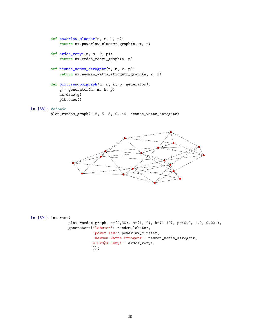
![In [40]: from IPython.html.widgets import interact import matplotlib.pyplot as plt](https://files.speakerdeck.com/presentations/969ec830302c013297b132228b43df58/slide_20.jpg)
![12 Machine Learning with Sci-Kit Learn In [44]: solve =](https://files.speakerdeck.com/presentations/969ec830302c013297b132228b43df58/slide_22.jpg)
![• LATEX • Reveal.js slideshow In []: !ipython nbconvert pyconza_ipython.ipynb](https://files.speakerdeck.com/presentations/969ec830302c013297b132228b43df58/slide_25.jpg)