Department of Earth and Environmental Science Instructors Ryan Abernathey ([email protected]) TA: Xiaomeng Jin ([email protected]) Meeting Time Tuesday / Thursday 10:10am - 11:25am 506 Schermerhorn Prerequisites DEES grad student status or instructor permission. Access to a laptop. Website https://rabernat.github.io/research_computing_2018/
Simulations E 5 r 0 jUj p ðN/jUj jfj/jUj P 1D (k) ffiffiffiffiffiffiffiffiffiffiffiffiffiffiffiffiffiffiffiffiffiffiffiffiffi ffi N2 2 jUj2k2 q ffiffiffiffiffiffiffiffiffiffiffiffiffiffiffiffiffiffiffiffiffiffiffiffi jUj2k2 2 f2 q dk, (3) where k 5 (k, l) is now the wavenumber in the reference frame along and across the mean flow U and P 1D (k) 5 1 2p ð1‘ 2‘ jkj jkj P 2D (k, l) dl (4) is the effective one-dimensional (1D) topographic spectrum. Hence, the wave radiation from 2D topogra- phy reduces to an equivalent problem of wave radiation from 1D topography with the effective spectrum given by P1D (k). The effective 1D spectrum captures the effects of 2D topography on lee-wave radiation in the subcritical to- pography limit, that is, P2D (k, l) and P1D (k) result into identical radiation estimates for small steepness pa- rameters. However, the suppression of wave radiation in the critical topography limit is different in 1D and 2D; c. Bottom topography Simulations are configured with multiscale topogra- phy characterized by small-scale abyssal hills a few ki- lometers wide based on multibeam observations from Drake Passage. The topographic spectrum associated with abyssal hills is well described by an anisotropic parametric representation proposed by Goff and Jordan (1988): P 2D (k, l) 5 2pH2(m 2 2) k 0 l 0 1 1 k2 k2 0 1 l2 l2 0 !2m/2 , (5) where k0 and l0 set the wavenumbers of the large hills, m is the high-wavenumber spectral slope, related to the pa- rameter n used in Goff and Jordan (1988) as m 5 2(n 1 1), and H is the root-mean-square (rms) topographic height. Nikurashin and Ferrari (2010b) estimated with a least squares fit to multibeam data that representative values in the Drake Passage region are k0 5 2.3 3 1024 m21, l0 5 24 21 FIG. 3. Averaged profiles of (left) stratification (s21) and (right) flow speed (m s21) in the bottom 2 km from observations (gray), initial condition in the simulations (black), and final state in 2D (blue) and 3D (red) simulations.
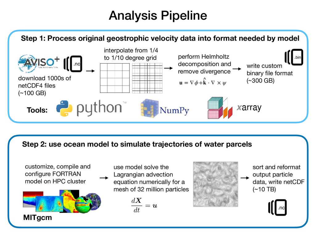
format needed by model download 1000s of netCDF4 files (~100 GB) .nc interpolate from 1/4 to 1/10 degree grid perform Helmholtz decomposition and remove divergence .bin write custom binary file format (~300 GB) Tools: Step 2: use ocean model to simulate trajectories of water parcels dX dt = u MITgcm customize, compile and configure FORTRAN model on HPC cluster use model solve the Lagrangian advection equation numerically for a mesh of 32 million particles sort and reformat output particle data, write netCDF (~10 TB) .nc
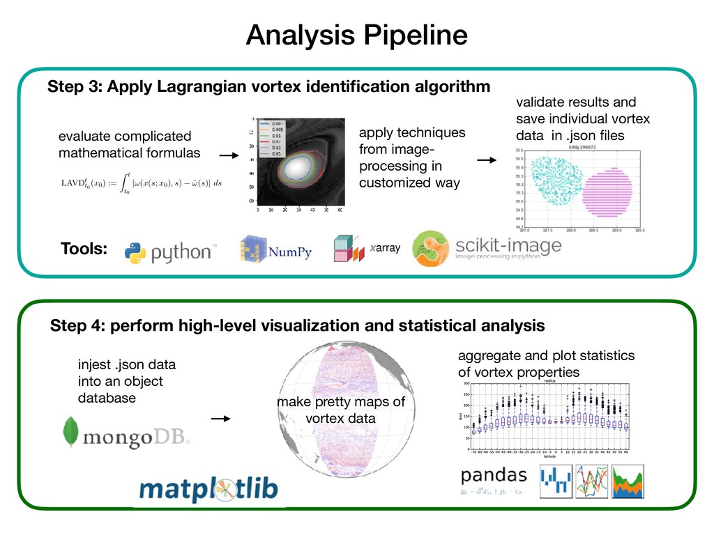
techniques from image- processing in customized way validate results and save individual vortex data in .json files Tools: Step 4: perform high-level visualization and statistical analysis injest .json data into an object database rotation tensor ⇥t t0 is not dynamically consistent because (16) exhibits the same memory ussed for (12). ynamic consistency of t t0 implies that the total angle swept by this tensor around its of rotation is dynamically consistent. This angle t t0 (x 0 ), called intrinsic rotation angle 1)), therefore satisfies t t0 (x 0 ) = t s (x 0 ) + s t0 (x 0 ), s, t 2 [t 0 , t 1 ]. on, as shown in Haller (2015b), t t0 (x 0 ) is objective both in two and three dimensions. In nsions, even the tensor t t0 itself turns out to be objective, not just its associated scalar 0 ). the results obtained in Haller (2015b), the intrinsic dynamic rotation t t0 (x 0 ) can be as t t0 (x 0 ) = 1 2 LAVDt t0 (x 0 ), (17) Lagrangian-Averaged Vorticity Deviation (LAVD) defined here as LAVDt t0 (x 0 ) := Z t t0 |!(x(s; x 0 ), s) ¯ !(s)| ds. (18) tivity of t t0 and LAVD can be confirmed directly from formula (6). Indeed, under a observer change x = Q(t)y + b(t), the transformed vorticity ˜ !(y, t) satisfies !(y(s), s) ˜ ¯ !(s)| = QT (s)!(x(s), s) + QT (t) ˙ q(t) QT (s)¯ !(s) + QT (t) ˙ q(t) = QT (s) [!(x(s), s) ¯ !(s)] = |!(x(s), s) ¯ !(s)| , (19) he rotation matrix QT (s) preserves the length of vectors. We summarize the results of n as follows: 1. For an infinitesimal fluid volume starting from x 0 , the LAVDt t0 (x 0 ) field is a dynami- stent and objective measure of bulk material rotation relative to the spatial mean-rotation d volume U(t). Specifically, LAVDt t0 (x 0 ) is twice the intrinsic dynamic rotation angle by the relative rotation tensor t t0 . The latter tensor is obtained from the dynamically decomposition Ft t0 = t t0 ⇥t t0 Mt t0 (20) 6 evaluate complicated mathematical formulas make pretty maps of vortex data aggregate and plot statistics of vortex properties
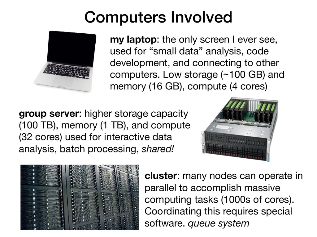
used for “small data” analysis, code development, and connecting to other computers. Low storage (~100 GB) and memory (16 GB), compute (4 cores) group server: higher storage capacity (100 TB), memory (1 TB), and compute (32 cores) used for interactive data analysis, batch processing, shared! cluster: many nodes can operate in parallel to accomplish massive computing tasks (1000s of cores). Coordinating this requires special software. queue system
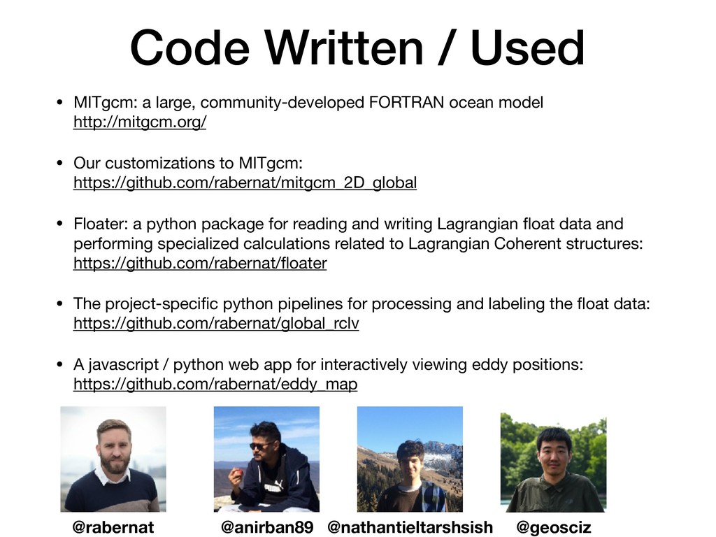
ocean model http://mitgcm.org/ • Our customizations to MITgcm: https://github.com/rabernat/mitgcm_2D_global • Floater: a python package for reading and writing Lagrangian float data and performing specialized calculations related to Lagrangian Coherent structures: https://github.com/rabernat/floater • The project-specific python pipelines for processing and labeling the float data: https://github.com/rabernat/global_rclv • A javascript / python web app for interactively viewing eddy positions: https://github.com/rabernat/eddy_map @rabernat @anirban89 @nathantieltarshsish @geosciz
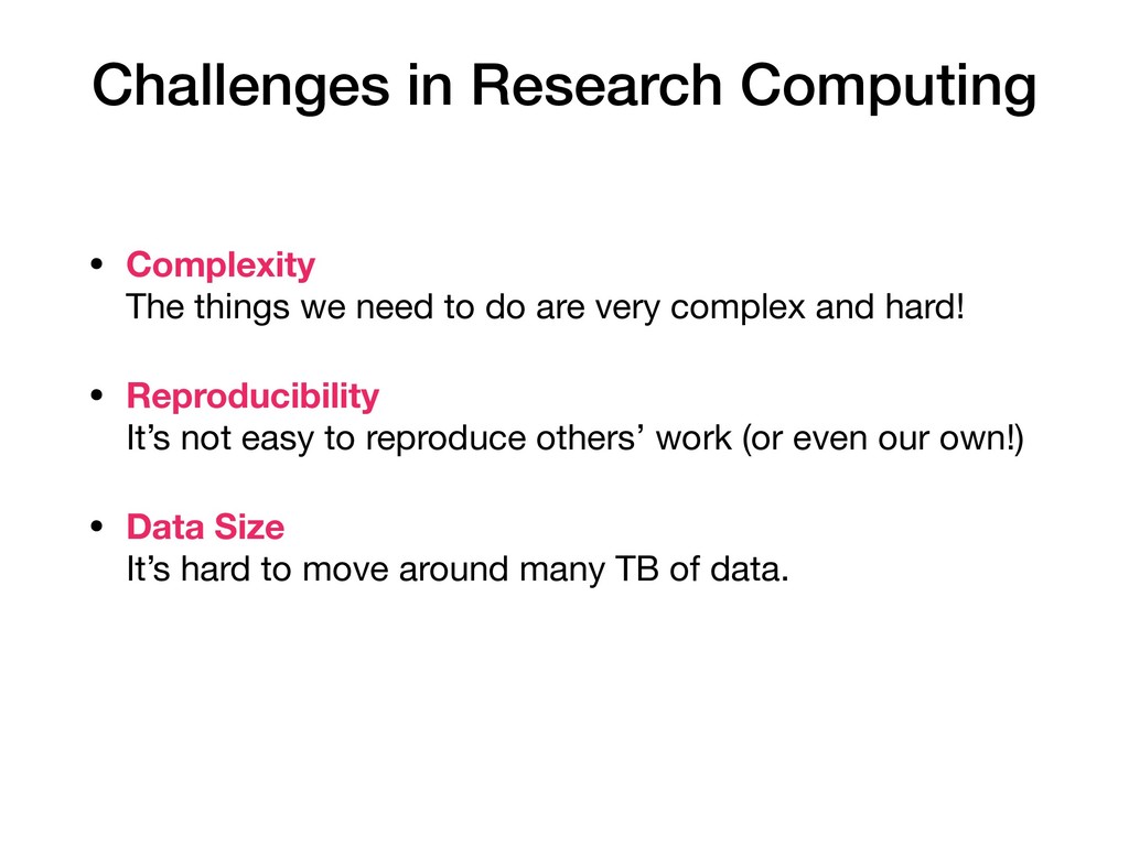
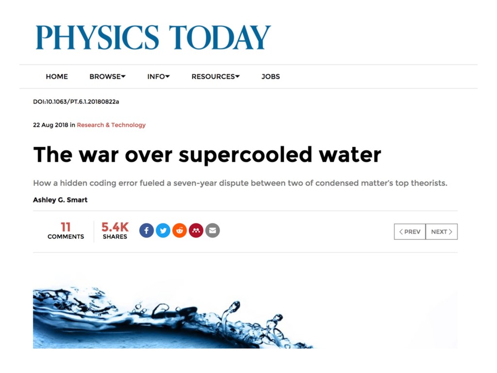
to do are very complex and hard! • Reproducibility It’s not easy to reproduce others’ work (or even our own!) • Data Size It’s hard to move around many TB of data.
analysis, Comp. Sci. Eng. 11(1):8–18, doi: 10.1109/MCSE.2009.15 “an article about computational science … is not the scholarship itself, it’s merely scholarship advertisement. The actual scholarship is the complete software development environment and the complete set of instructions which generated the figures.”
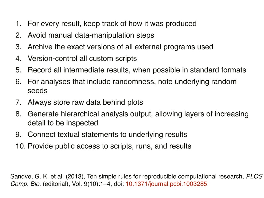
produced 2. Avoid manual data-manipulation steps 3. Archive the exact versions of all external programs used 4. Version-control all custom scripts 5. Record all intermediate results, when possible in standard formats 6. For analyses that include randomness, note underlying random seeds 7. Always store raw data behind plots 8. Generate hierarchical analysis output, allowing layers of increasing detail to be inspected 9. Connect textual statements to underlying results 10. Provide public access to scripts, runs, and results Sandve, G. K. et al. (2013), Ten simple rules for reproducible computational research, PLOS Comp. Bio. (editorial), Vol. 9(10):1–4, doi: 10.1371/journal.pcbi.1003285
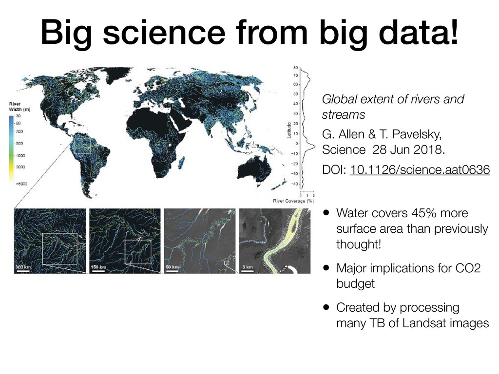
streams G. Allen & T. Pavelsky, Science 28 Jun 2018. DOI: 10.1126/science.aat0636 • Water covers 45% more surface area than previously thought! • Major implications for CO2 budget • Created by processing many TB of Landsat images
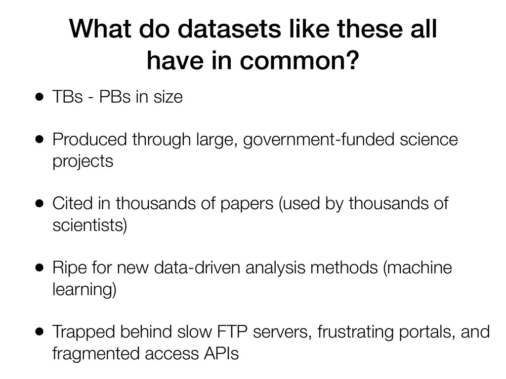
TBs - PBs in size • Produced through large, government-funded science projects • Cited in thousands of papers (used by thousands of scientists) • Ripe for new data-driven analysis methods (machine learning) • Trapped behind slow FTP servers, frustrating portals, and fragmented access APIs
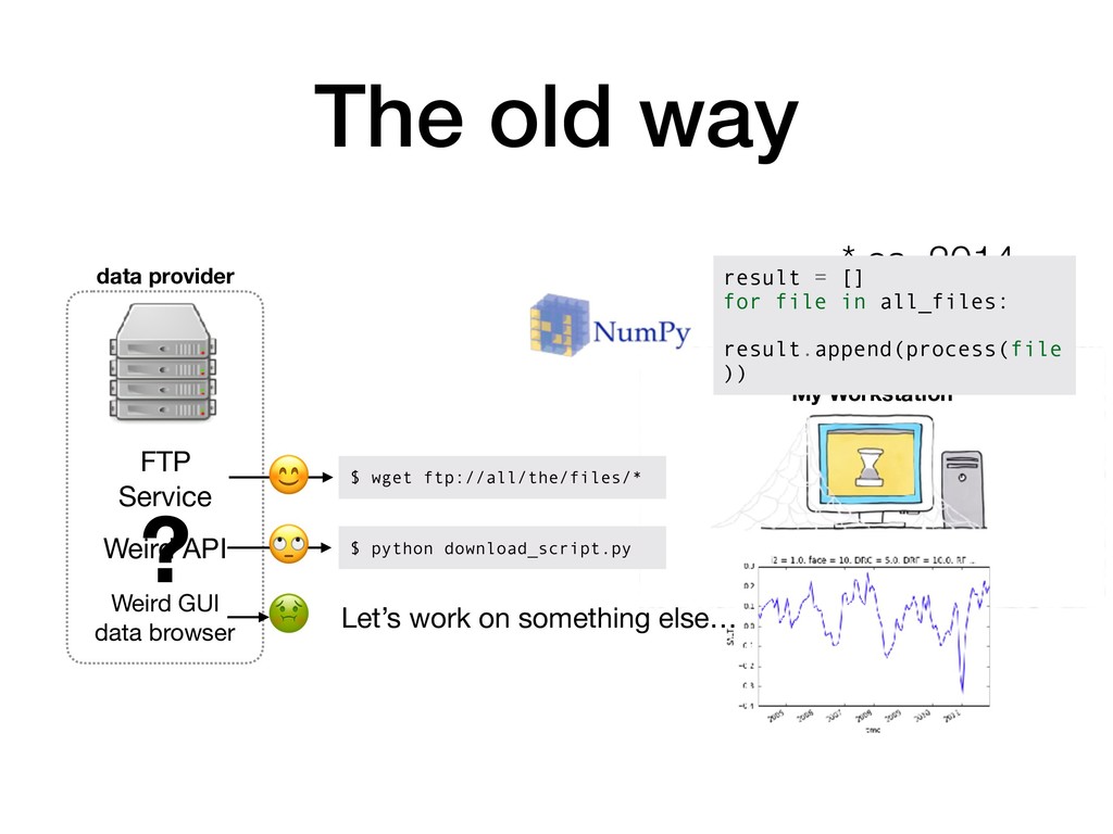
$ python download_script.py Weird API Weird GUI data browser Let’s work on something else… ? My Workstation * ca. 2014 result = [] for file in all_files: result.append(process(file ))
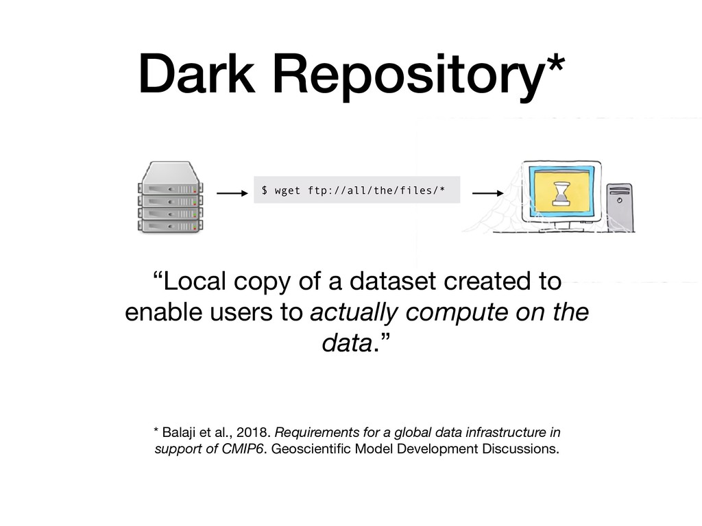
Requirements for a global data infrastructure in support of CMIP6. Geoscientific Model Development Discussions. “Local copy of a dataset created to enable users to actually compute on the data.”
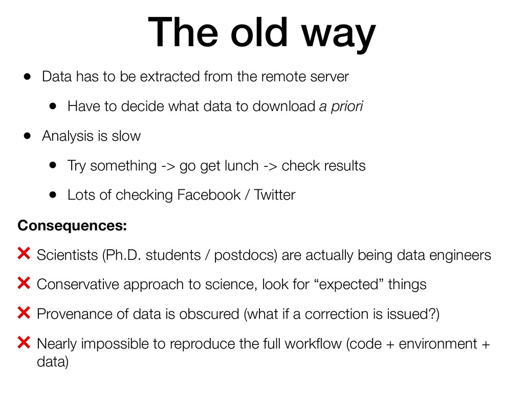
• Have to decide what data to download a priori • Analysis is slow • Try something -> go get lunch -> check results • Lots of checking Facebook / Twitter The old way Consequences: ❌ Scientists (Ph.D. students / postdocs) are actually being data engineers ❌ Conservative approach to science, look for “expected” things ❌ Provenance of data is obscured (what if a correction is issued?) ❌ Nearly impossible to reproduce the full workflow (code + environment + data)
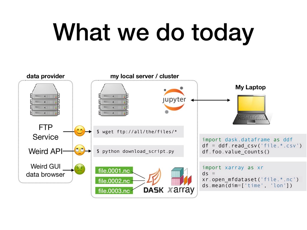
ftp://all/the/files/* my local server / cluster $ python download_script.py Weird API Weird GUI data browser file.0001.nc file.0002.nc file.0003.nc My Laptop import dask.dataframe as ddf df = ddf.read_csv('file.*.csv') df.foo.value_counts() import xarray as xr ds = xr.open_mfdataset('file.*.nc') ds.mean(dim=[‘time', ‘lon'])
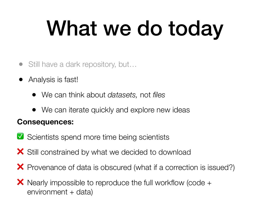
but… • Analysis is fast! • We can think about datasets, not files • We can iterate quickly and explore new ideas Consequences: ✅ Scientists spend more time being scientists ❌ Still constrained by what we decided to download ❌ Provenance of data is obscured (what if a correction is issued?) ❌ Nearly impossible to reproduce the full workflow (code + environment + data)
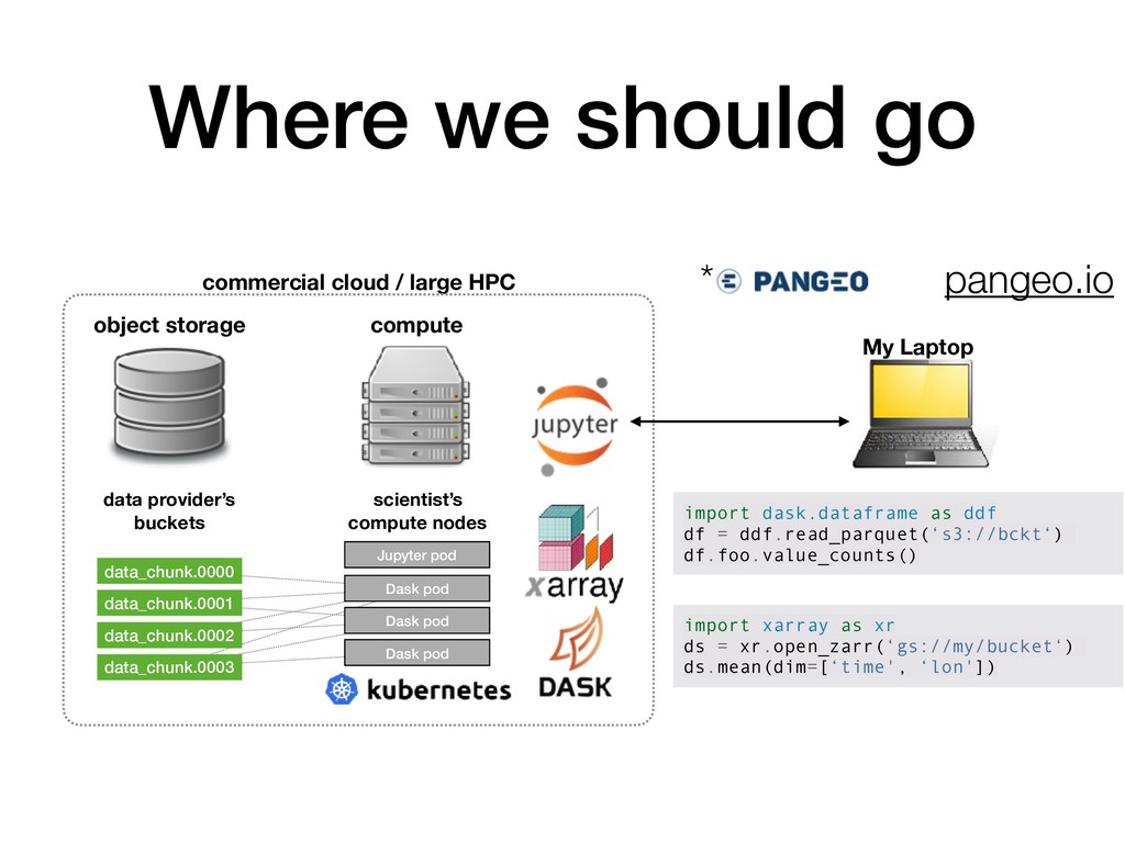
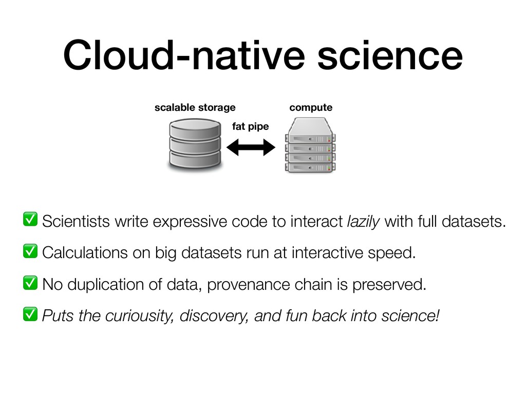
datasets. ✅ Calculations on big datasets run at interactive speed. ✅ No duplication of data, provenance chain is preserved. ✅ Puts the curiousity, discovery, and fun back into science! Cloud-native science scalable storage compute fat pipe
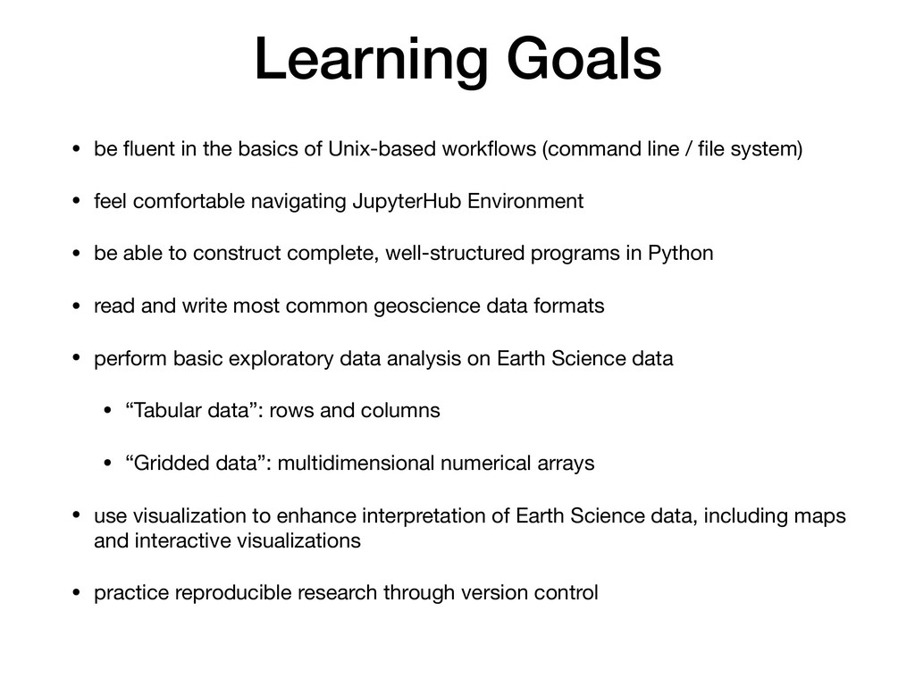
workflows (command line / file system) • feel comfortable navigating JupyterHub Environment • be able to construct complete, well-structured programs in Python • read and write most common geoscience data formats • perform basic exploratory data analysis on Earth Science data • “Tabular data”: rows and columns • “Gridded data”: multidimensional numerical arrays • use visualization to enhance interpretation of Earth Science data, including maps and interactive visualizations • practice reproducible research through version control
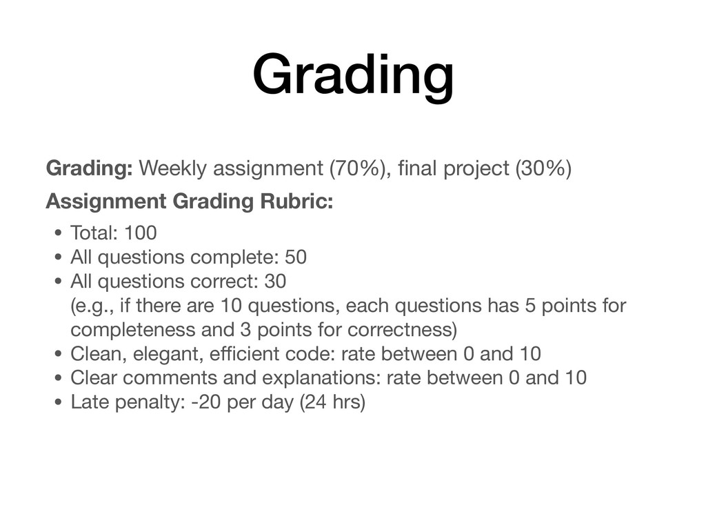
Rubric: • Total: 100 • All questions complete: 50 • All questions correct: 30 (e.g., if there are 10 questions, each questions has 5 points for completeness and 3 points for correctness) • Clean, elegant, efficient code: rate between 0 and 10 • Clear comments and explanations: rate between 0 and 10 • Late penalty: -20 per day (24 hrs)
of the programming languages covered in this course to carry out an extensive data analysis, modeling or visualization task. • You will be required to briefly present and demo your final project during the last week of classes. • More details to be given soon.
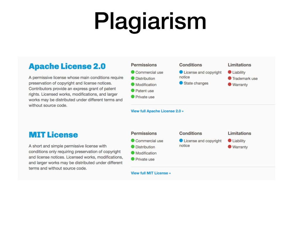
of others. It comes from the Latin word plagiaries, meaning ‘kidnapper’.” - https://www.college.columbia.edu/ academics/academicdishonesty • Copying someone else's code and turning it in as your own work for an assignment or for the final project is plagiarism • You will receive 0 credit for plagiarized work • However, open source software is all about reuse. The key is the License: https://choosealicense.com/licenses/ • Since the purpose of this course is to teach you how to program, you are required to write your own original codes for the assignments and final project.
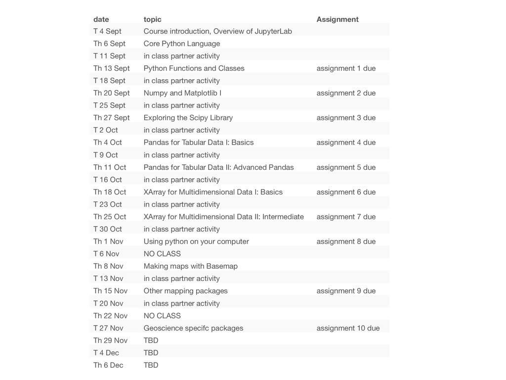
JupyterLab Th 6 Sept Core Python Language T 11 Sept in class partner activity Th 13 Sept Python Functions and Classes assignment 1 due T 18 Sept in class partner activity Th 20 Sept Numpy and Matplotlib I assignment 2 due T 25 Sept in class partner activity Th 27 Sept Exploring the Scipy Library assignment 3 due T 2 Oct in class partner activity Th 4 Oct Pandas for Tabular Data I: Basics assignment 4 due T 9 Oct in class partner activity Th 11 Oct Pandas for Tabular Data II: Advanced Pandas assignment 5 due T 16 Oct in class partner activity Th 18 Oct XArray for Multidimensional Data I: Basics assignment 6 due T 23 Oct in class partner activity Th 25 Oct XArray for Multidimensional Data II: Intermediate assignment 7 due T 30 Oct in class partner activity Th 1 Nov Using python on your computer assignment 8 due T 6 Nov NO CLASS Th 8 Nov Making maps with Basemap T 13 Nov in class partner activity Th 15 Nov Other mapping packages assignment 9 due T 20 Nov in class partner activity Th 22 Nov NO CLASS T 27 Nov Geoscience specifc packages assignment 10 due Th 29 Nov TBD T 4 Dec TBD Th 6 Dec TBD
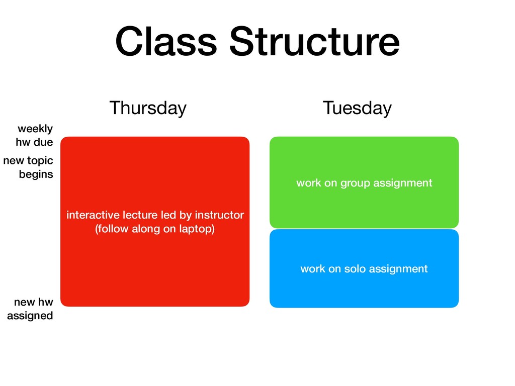
how to code is to start coding, so bring your laptop to class so you can be practicing the various coding commands while we present them. You will also need your laptop to work on the assignments during the in- class activity days.