Lecture 6 - Stochastic population models

Transcript

1. Stochasticity
2. Today’s topics 1 Introduction 2 Geometric Growth 3 Logistic growth
3. Random Variables A random variable is a variable whose value can’t be predicted with certainty. Introduction Geometric Growth Logistic growth 3 / 17
4. Random Variables A random variable is a variable whose value can’t be predicted with certainty. Examples? • Weather • Our own behavior • Population size Introduction Geometric Growth Logistic growth 3 / 17
5. Probability distributions A random variable (X) can be described by a probability distribution. Introduction Geometric Growth Logistic growth 4 / 17
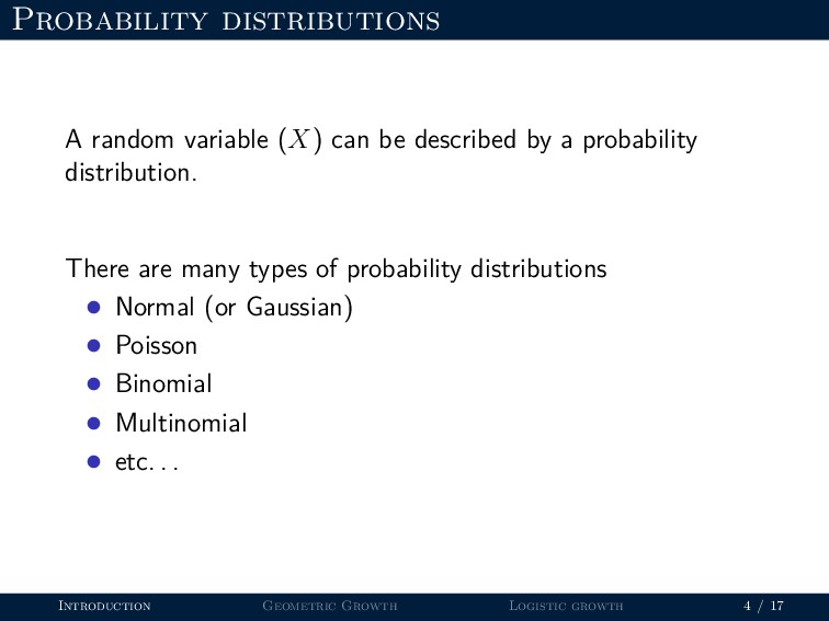
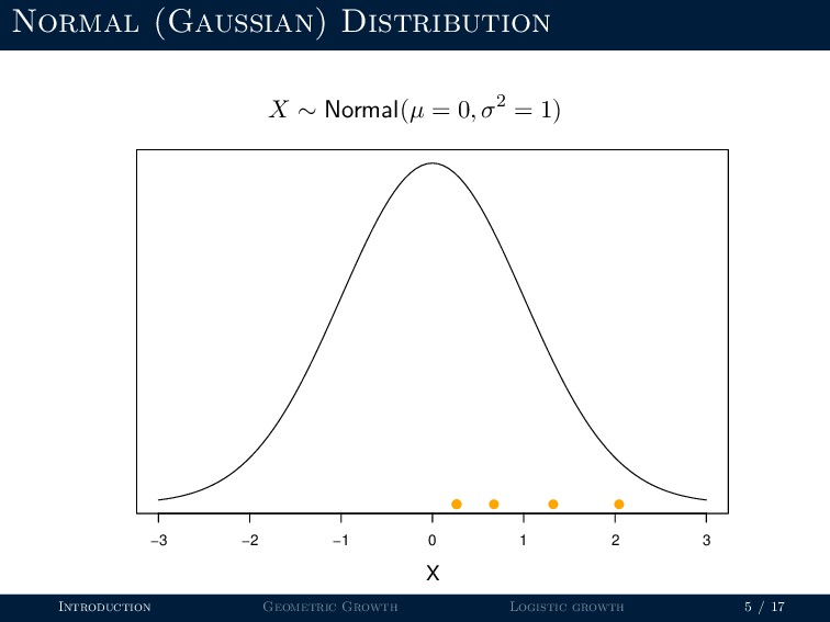
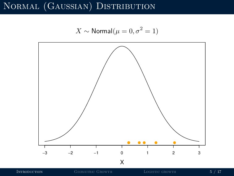
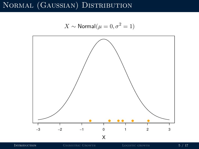
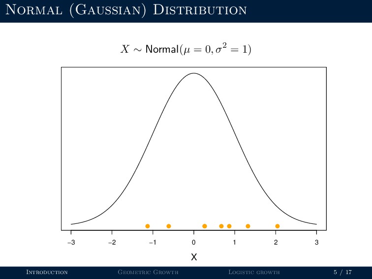
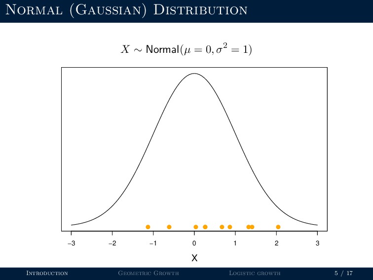
6. Probability distributions A random variable (X) can be described by a probability distribution. There are many types of probability distributions • Normal (or Gaussian) • Poisson • Binomial • Multinomial • etc. . . Introduction Geometric Growth Logistic growth 4 / 17
7. Normal (Gaussian) Distribution X ∼ Normal(µ = 0, σ2 = 1) −3 −2 −1 0 1 2 3 X Introduction Geometric Growth Logistic growth 5 / 17
8. Normal (Gaussian) Distribution X ∼ Normal(µ = 0, σ2 = 1) −3 −2 −1 0 1 2 3 X q Introduction Geometric Growth Logistic growth 5 / 17
9. Normal (Gaussian) Distribution X ∼ Normal(µ = 0, σ2 = 1) −3 −2 −1 0 1 2 3 X q q Introduction Geometric Growth Logistic growth 5 / 17
10. Normal (Gaussian) Distribution X ∼ Normal(µ = 0, σ2 = 1) −3 −2 −1 0 1 2 3 X q q q Introduction Geometric Growth Logistic growth 5 / 17
11. Normal (Gaussian) Distribution X ∼ Normal(µ = 0, σ2 = 1) −3 −2 −1 0 1 2 3 X q q q q Introduction Geometric Growth Logistic growth 5 / 17
12. Normal (Gaussian) Distribution X ∼ Normal(µ = 0, σ2 = 1) −3 −2 −1 0 1 2 3 X q q q q q Introduction Geometric Growth Logistic growth 5 / 17
13. Normal (Gaussian) Distribution X ∼ Normal(µ = 0, σ2 = 1) −3 −2 −1 0 1 2 3 X q q q q q q Introduction Geometric Growth Logistic growth 5 / 17
14. Normal (Gaussian) Distribution X ∼ Normal(µ = 0, σ2 = 1) −3 −2 −1 0 1 2 3 X q q q q q q q Introduction Geometric Growth Logistic growth 5 / 17
15. Normal (Gaussian) Distribution X ∼ Normal(µ = 0, σ2 = 1) −3 −2 −1 0 1 2 3 X q q q q q q q q Introduction Geometric Growth Logistic growth 5 / 17
16. Normal (Gaussian) Distribution X ∼ Normal(µ = 0, σ2 = 1) −3 −2 −1 0 1 2 3 X q q q q q q q q q Introduction Geometric Growth Logistic growth 5 / 17
17. Normal (Gaussian) Distribution X ∼ Normal(µ = 0, σ2 = 1) −3 −2 −1 0 1 2 3 X q q q q q q q q q q Introduction Geometric Growth Logistic growth 5 / 17
18. Normal (Gaussian) Distribution −2 −1 0 1 2 0.0 0.5 1.0 1.5 2.0 2.5 3.0 X Relative probability µ=0, σ2=0.6 µ=0, σ2=0.4 µ=0, σ2=0.2 Introduction Geometric Growth Logistic growth 6 / 17
19. A purely stochastic model Nt ∼ Normal(µ = 50, σ2 = 1) qq q q q q q q q q q q q q q q q qqq q q q q q q q q q q q q q q q q q q q q q q q q q q q q q q q q q q q q q q q q q q q q q q q q qqq q q q q q q q q q q q q q q q q q q q qq q q q q qq q q 0 20 40 60 80 100 48 49 50 51 52 Time Population size (N) Introduction Geometric Growth Logistic growth 7 / 17
20. Two important types of stochasticity Environmental stochasticity • Random variation in weather, habitat, etc. . . among years Introduction Geometric Growth Logistic growth 8 / 17
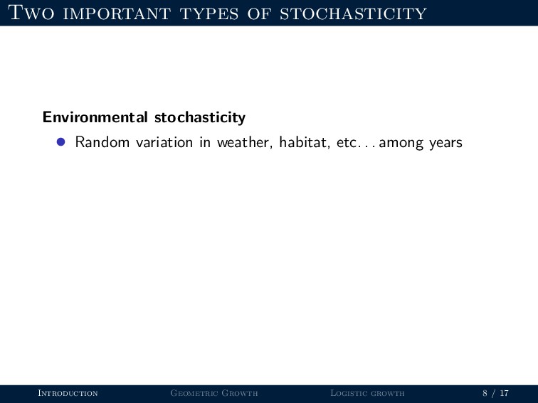
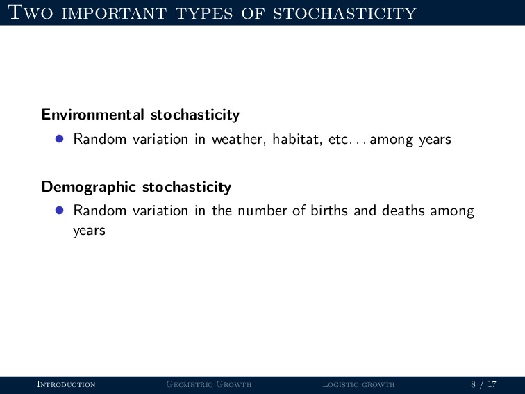
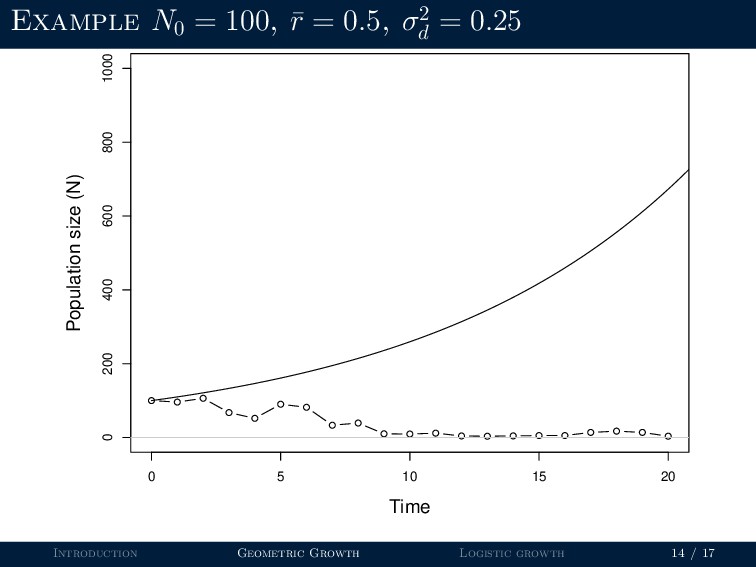
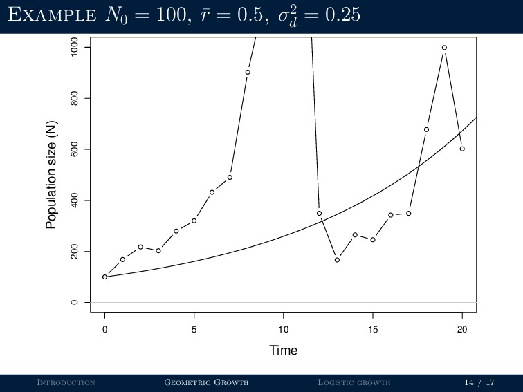
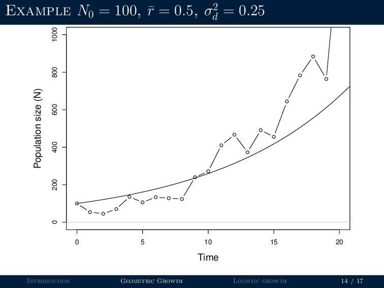
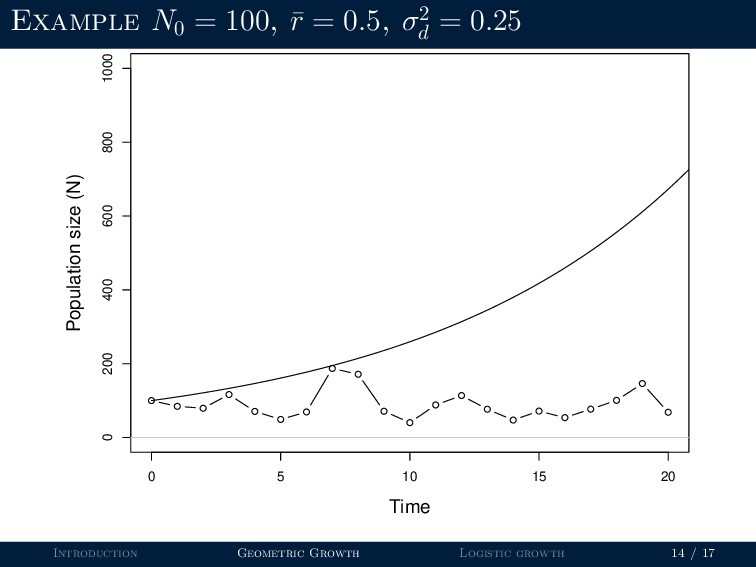
21. Two important types of stochasticity Environmental stochasticity • Random variation in weather, habitat, etc. . . among years Demographic stochasticity • Random variation in the number of births and deaths among years Introduction Geometric Growth Logistic growth 8 / 17
22. Geometric growth with environmental stochasticity Nt+1 = Nt + Nt r + Xt where Xt ∼ Normal(0, σ2 e ) Introduction Geometric Growth Logistic growth 9 / 17
23. Geometric growth with environmental stochasticity Nt+1 = Nt + Nt r + Xt where Xt ∼ Normal(0, σ2 e ) R code: r <- 0.1 sigma.e <- 10 for(t in 2:nYears) { X[t-1] <- rnorm(n=1, mean=0, sd=sigma.e) N[t] <- N[t-1] + N[t-1]*r + X[t-1] } Introduction Geometric Growth Logistic growth 9 / 17
24. Example N0 = 100, r = 0.1, µ = 0, σ2 e = 100 q q q q q q q q q q q q q q q q q q q q q 0 5 10 15 20 0 200 400 600 800 1000 Time Population size (N) Introduction Geometric Growth Logistic growth 10 / 17
25. Example N0 = 100, r = 0.1, µ = 0, σ2 e = 100 q q q q q q q q q q q q q q q q q q q q q 0 5 10 15 20 0 200 400 600 800 1000 Time Population size (N) Introduction Geometric Growth Logistic growth 10 / 17
26. Example N0 = 100, r = 0.1, µ = 0, σ2 e = 100 q q q q q q q q q q q q q q q q q q q q q 0 5 10 15 20 0 200 400 600 800 1000 Time Population size (N) Introduction Geometric Growth Logistic growth 10 / 17
27. Example N0 = 100, r = 0.1, µ = 0, σ2 e = 100 q q q q q q q q q q q q q q q q q q q q q 0 5 10 15 20 0 200 400 600 800 1000 Time Population size (N) Introduction Geometric Growth Logistic growth 10 / 17
28. Example N0 = 100, r = 0.1, µ = 0, σ2 e = 100 q q q q q q q q q q q q q q q q q q q q q 0 5 10 15 20 0 200 400 600 800 1000 Time Population size (N) Introduction Geometric Growth Logistic growth 10 / 17
29. Example N0 = 100, r = 0.1, µ = 0, σ2 e = 100 q q q q q q q q q q q q q q q q q q q q q 0 5 10 15 20 0 200 400 600 800 1000 Time Population size (N) Introduction Geometric Growth Logistic growth 10 / 17
30. Example N0 = 100, r = 0.1, µ = 0, σ2 e = 100 q q q q q q q q q q q q q q q q q q q q q 0 5 10 15 20 0 200 400 600 800 1000 Time Population size (N) Introduction Geometric Growth Logistic growth 10 / 17
31. Example N0 = 100, r = 0.1, µ = 0, σ2 e = 100 q q q q q q q q q q q q q q q q q q q q q 0 5 10 15 20 0 200 400 600 800 1000 Time Population size (N) Introduction Geometric Growth Logistic growth 10 / 17
32. Example N0 = 100, r = 0.1, µ = 0, σ2 e = 100 q q q q q q q q q q q q q q q q q q q q q 0 5 10 15 20 0 200 400 600 800 1000 Time Population size (N) Introduction Geometric Growth Logistic growth 10 / 17
33. Example N0 = 100, r = 0.1, µ = 0, σ2 e = 100 q q q q q q q q q q q q q q q q q q q q q 0 5 10 15 20 0 200 400 600 800 1000 Time Population size (N) Introduction Geometric Growth Logistic growth 10 / 17
34. Example N0 = 100, r = 0.1, µ = 0, σ2 e = 10000 q q q q q q q q q q q q q q q q q q 0 5 10 15 20 0 200 400 600 800 1000 Time Population size (N) Introduction Geometric Growth Logistic growth 11 / 17
35. Example N0 = 100, r = 0.1, µ = 0, σ2 e = 10000 q q q q q q q q q q q q q q q q q q q q q 0 5 10 15 20 0 200 400 600 800 1000 Time Population size (N) Introduction Geometric Growth Logistic growth 11 / 17
36. Example N0 = 100, r = 0.1, µ = 0, σ2 e = 10000 q q q q q q q q q q q q q q q q q q q q q 0 5 10 15 20 0 200 400 600 800 1000 Time Population size (N) Introduction Geometric Growth Logistic growth 11 / 17
37. Example N0 = 100, r = 0.1, µ = 0, σ2 e = 10000 q q q q q q q q q q q q 0 5 10 15 20 0 200 400 600 800 1000 Time Population size (N) Introduction Geometric Growth Logistic growth 11 / 17
38. Example N0 = 100, r = 0.1, µ = 0, σ2 e = 10000 q q q q q q q q q q q q q q q q q q q q q 0 5 10 15 20 0 200 400 600 800 1000 Time Population size (N) Introduction Geometric Growth Logistic growth 11 / 17
39. Example N0 = 100, r = 0.1, µ = 0, σ2 e = 10000 q q q q q q q q q q q q q q q q q q q q q 0 5 10 15 20 0 200 400 600 800 1000 Time Population size (N) Introduction Geometric Growth Logistic growth 11 / 17
40. Example N0 = 100, r = 0.1, µ = 0, σ2 e = 10000 q q q q q q q q q q q q q q q q q q q 0 5 10 15 20 0 200 400 600 800 1000 Time Population size (N) Introduction Geometric Growth Logistic growth 11 / 17
41. Example N0 = 100, r = 0.1, µ = 0, σ2 e = 10000 q q q q q q q q q q q q q q q q q q q q q 0 5 10 15 20 0 200 400 600 800 1000 Time Population size (N) Introduction Geometric Growth Logistic growth 11 / 17
42. Example N0 = 100, r = 0.1, µ = 0, σ2 e = 10000 q q q q q q q q q q q q q q q q q q q q q 0 5 10 15 20 0 200 400 600 800 1000 Time Population size (N) Introduction Geometric Growth Logistic growth 11 / 17
43. Example N0 = 100, r = 0.1, µ = 0, σ2 e = 10000 q q q q q q q q q 0 5 10 15 20 0 200 400 600 800 1000 Time Population size (N) Introduction Geometric Growth Logistic growth 11 / 17
44. Geometric growth with demographic stochasticity Nt+1 = Nt + Nt rt Introduction Geometric Growth Logistic growth 12 / 17
45. Geometric growth with demographic stochasticity Nt+1 = Nt + Nt rt where rt ∼ Normal(¯ r, σ2 d ) Introduction Geometric Growth Logistic growth 12 / 17
46. Example N0 = 100, ¯ r = 0.5, σ2 d = 0.01 q q q q q q q q q q q q q q q q q q q q q 0 5 10 15 20 0 200 400 600 800 1000 Time Population size (N) Introduction Geometric Growth Logistic growth 13 / 17
47. Example N0 = 100, ¯ r = 0.5, σ2 d = 0.01 q q q q q q q q q q q q q q q q q q q q q 0 5 10 15 20 0 200 400 600 800 1000 Time Population size (N) Introduction Geometric Growth Logistic growth 13 / 17
48. Example N0 = 100, ¯ r = 0.5, σ2 d = 0.01 q q q q q q q q q q q q q q q q q q q q q 0 5 10 15 20 0 200 400 600 800 1000 Time Population size (N) Introduction Geometric Growth Logistic growth 13 / 17
49. Example N0 = 100, ¯ r = 0.5, σ2 d = 0.01 q q q q q q q q q q q q q q q q q q q q q 0 5 10 15 20 0 200 400 600 800 1000 Time Population size (N) Introduction Geometric Growth Logistic growth 13 / 17
50. Example N0 = 100, ¯ r = 0.5, σ2 d = 0.01 q q q q q q q q q q q q q q q q q q q q q 0 5 10 15 20 0 200 400 600 800 1000 Time Population size (N) Introduction Geometric Growth Logistic growth 13 / 17
51. Example N0 = 100, ¯ r = 0.5, σ2 d = 0.01 q q q q q q q q q q q q q q q q q q q q q 0 5 10 15 20 0 200 400 600 800 1000 Time Population size (N) Introduction Geometric Growth Logistic growth 13 / 17
52. Example N0 = 100, ¯ r = 0.5, σ2 d = 0.01 q q q q q q q q q q q q q q q q q q q q q 0 5 10 15 20 0 200 400 600 800 1000 Time Population size (N) Introduction Geometric Growth Logistic growth 13 / 17
53. Example N0 = 100, ¯ r = 0.5, σ2 d = 0.01 q q q q q q q q q q q q q q q q q q q q q 0 5 10 15 20 0 200 400 600 800 1000 Time Population size (N) Introduction Geometric Growth Logistic growth 13 / 17
54. Example N0 = 100, ¯ r = 0.5, σ2 d = 0.01 q q q q q q q q q q q q q q q q q q q q q 0 5 10 15 20 0 200 400 600 800 1000 Time Population size (N) Introduction Geometric Growth Logistic growth 13 / 17
55. Example N0 = 100, ¯ r = 0.5, σ2 d = 0.01 q q q q q q q q q q q q q q q q q q q q q 0 5 10 15 20 0 200 400 600 800 1000 Time Population size (N) Introduction Geometric Growth Logistic growth 13 / 17
56. Example N0 = 100, ¯ r = 0.5, σ2 d = 0.25 q q q q q q q q q q q q q q q q q q q q q 0 5 10 15 20 0 200 400 600 800 1000 Time Population size (N) Introduction Geometric Growth Logistic growth 14 / 17
57. Example N0 = 100, ¯ r = 0.5, σ2 d = 0.25 q q q q q q q q q q q q q q q q q q q q q 0 5 10 15 20 0 200 400 600 800 1000 Time Population size (N) Introduction Geometric Growth Logistic growth 14 / 17
58. Example N0 = 100, ¯ r = 0.5, σ2 d = 0.25 q q q q q q q q q q q q q q q q q q q q q 0 5 10 15 20 0 200 400 600 800 1000 Time Population size (N) Introduction Geometric Growth Logistic growth 14 / 17
59. Example N0 = 100, ¯ r = 0.5, σ2 d = 0.25 q q q q q q q q q q q q q q q q q q q q q 0 5 10 15 20 0 200 400 600 800 1000 Time Population size (N) Introduction Geometric Growth Logistic growth 14 / 17
60. Example N0 = 100, ¯ r = 0.5, σ2 d = 0.25 q q q q q q q q q q q q q q q q q q q q q 0 5 10 15 20 0 200 400 600 800 1000 Time Population size (N) Introduction Geometric Growth Logistic growth 14 / 17
61. Example N0 = 100, ¯ r = 0.5, σ2 d = 0.25 q q q q q q q q q q q q q q q q q q 0 5 10 15 20 0 200 400 600 800 1000 Time Population size (N) Introduction Geometric Growth Logistic growth 14 / 17
62. Example N0 = 100, ¯ r = 0.5, σ2 d = 0.25 q q q q q q q q q q q q q q q q q q q q 0 5 10 15 20 0 200 400 600 800 1000 Time Population size (N) Introduction Geometric Growth Logistic growth 14 / 17
63. Example N0 = 100, ¯ r = 0.5, σ2 d = 0.25 q q q q q q q q q q q q q q q q q q q q q 0 5 10 15 20 0 200 400 600 800 1000 Time Population size (N) Introduction Geometric Growth Logistic growth 14 / 17
64. Example N0 = 100, ¯ r = 0.5, σ2 d = 0.25 q q q q q q q q q q q q q q q q q q q q q 0 5 10 15 20 0 200 400 600 800 1000 Time Population size (N) Introduction Geometric Growth Logistic growth 14 / 17
65. Example N0 = 100, ¯ r = 0.5, σ2 d = 0.25 q q q q q q q q q q q q q q q q q q q q q 0 5 10 15 20 0 200 400 600 800 1000 Time Population size (N) Introduction Geometric Growth Logistic growth 14 / 17
66. Logistic growth with stochastic carrying capacity Nt+1 = Nt + Nt rmax (1 − Nt /Kt ) where Kt ∼ Normal( ¯ K, σ2 e ) Introduction Geometric Growth Logistic growth 15 / 17
67. Logistic example, rmax = 0.2, ¯ K = 100, σ2 e = 400 q q q q q q q q q q q q q q q q q q q q q 0 5 10 15 20 0 50 100 150 200 250 300 Time Population size (N) Introduction Geometric Growth Logistic growth 16 / 17
68. Logistic example, rmax = 0.2, ¯ K = 100, σ2 e = 400 q q q q q q q q q q q q q q q q q q q q q 0 5 10 15 20 0 50 100 150 200 250 300 Time Population size (N) Introduction Geometric Growth Logistic growth 16 / 17
69. Logistic example, rmax = 0.2, ¯ K = 100, σ2 e = 400 q q q q q q q q q q q q q q q q q q q q q 0 5 10 15 20 0 50 100 150 200 250 300 Time Population size (N) Introduction Geometric Growth Logistic growth 16 / 17
70. Logistic example, rmax = 0.2, ¯ K = 100, σ2 e = 400 q q q q q q q q q q q q q q q q q q q q q 0 5 10 15 20 0 50 100 150 200 250 300 Time Population size (N) Introduction Geometric Growth Logistic growth 16 / 17
71. Logistic example, rmax = 0.2, ¯ K = 100, σ2 e = 400 q q q q q q q q q q q q q q q q q q q q q 0 5 10 15 20 0 50 100 150 200 250 300 Time Population size (N) Introduction Geometric Growth Logistic growth 16 / 17
72. Logistic example, rmax = 0.2, ¯ K = 100, σ2 e = 400 q q q q q q q q q q q q q q q q q q q q q 0 5 10 15 20 0 50 100 150 200 250 300 Time Population size (N) Introduction Geometric Growth Logistic growth 16 / 17
73. Logistic example, rmax = 0.2, ¯ K = 100, σ2 e = 400 q q q q q q q q q q q q q q q q q q q q q 0 5 10 15 20 0 50 100 150 200 250 300 Time Population size (N) Introduction Geometric Growth Logistic growth 16 / 17
74. Logistic example, rmax = 0.2, ¯ K = 100, σ2 e = 400 q q q q q q q q q q q q q q q q q q q q q 0 5 10 15 20 0 50 100 150 200 250 300 Time Population size (N) Introduction Geometric Growth Logistic growth 16 / 17
75. Logistic example, rmax = 0.2, ¯ K = 100, σ2 e = 400 q q q q q q q q q q q q q q q q q q q q q 0 5 10 15 20 0 50 100 150 200 250 300 Time Population size (N) Introduction Geometric Growth Logistic growth 16 / 17
76. Logistic example, rmax = 0.2, ¯ K = 100, σ2 e = 400 q q q q q q q q q q q q q q q q q q q q q 0 5 10 15 20 0 50 100 150 200 250 300 Time Population size (N) Introduction Geometric Growth Logistic growth 16 / 17
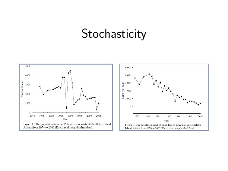
77. Summary Purely deterministic models are too rigid Purely stochastic models don’t tell us much The goal is to develop a mechanistic model that represents our biological understanding while allowing for stochasticity Introduction Geometric Growth Logistic growth 17 / 17