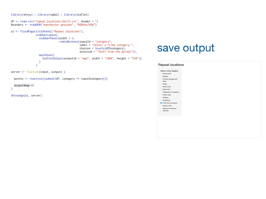
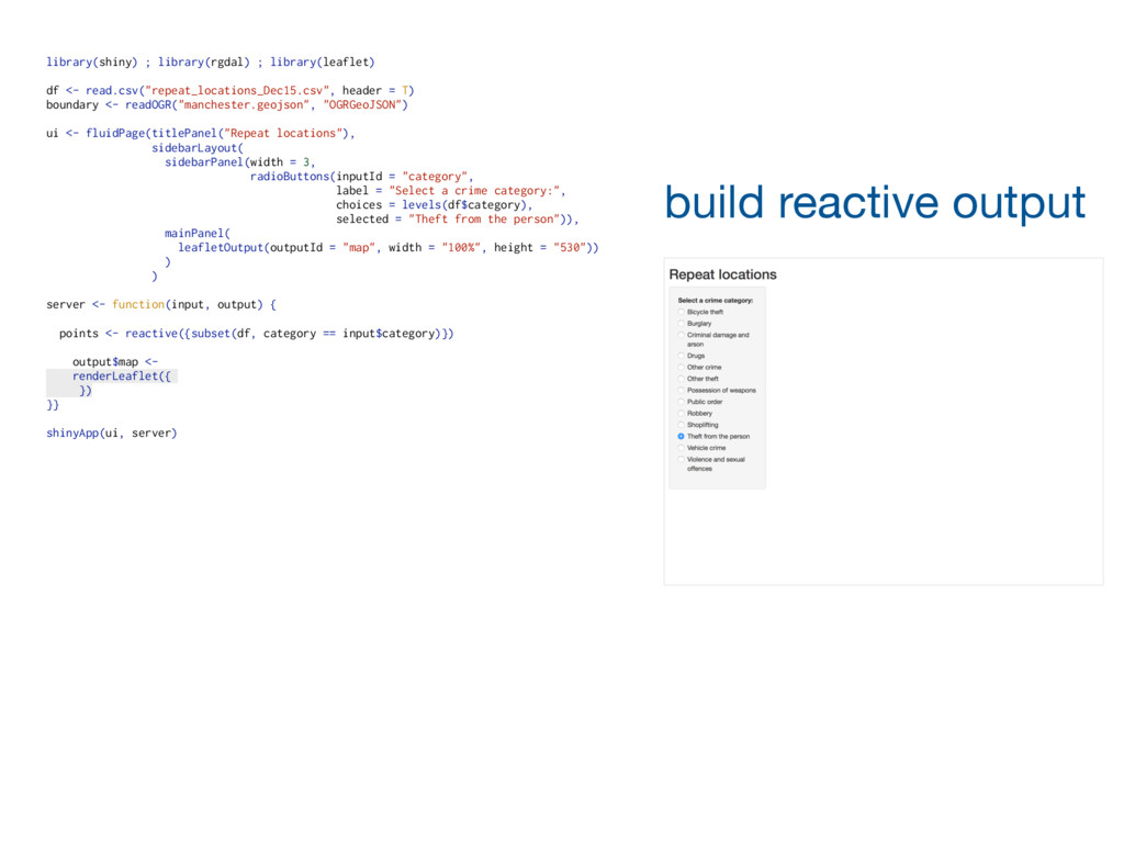
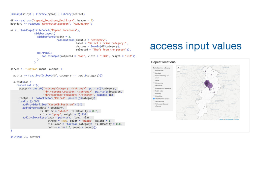
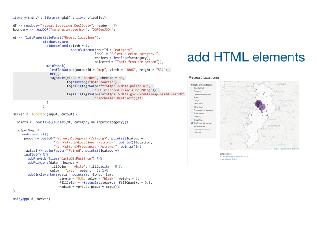
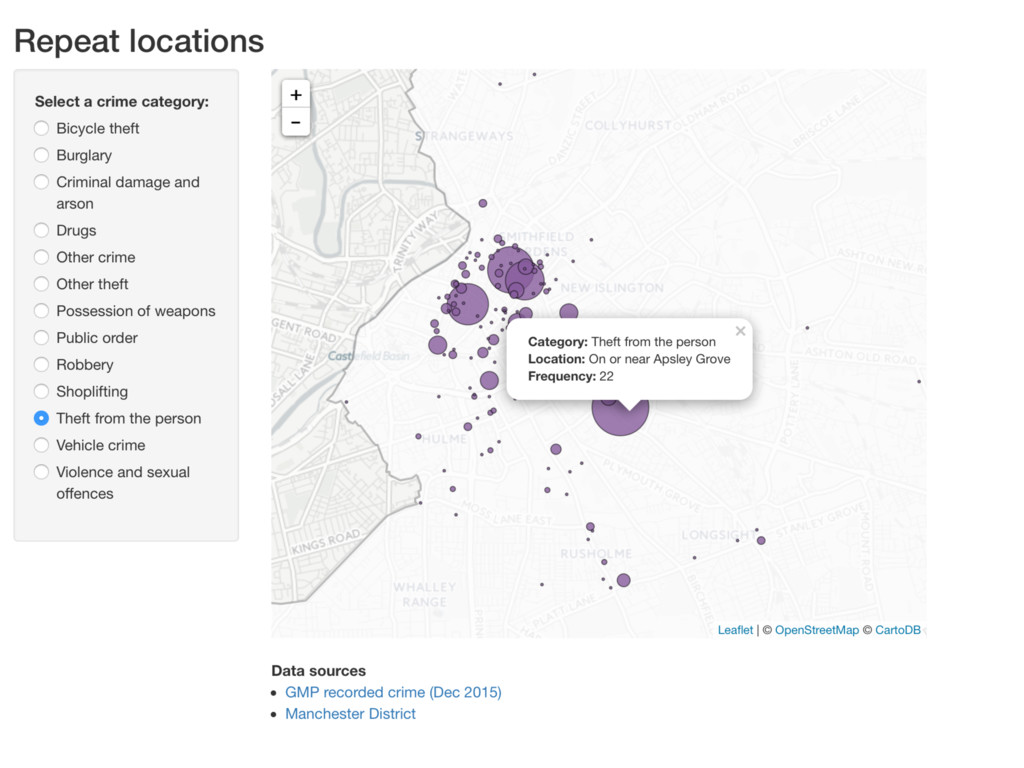
T) boundary <- readOGR("manchester.geojson", "OGRGeoJSON") ui <- fluidPage(titlePanel("Repeat locations"), sidebarLayout( sidebarPanel(width = 3, radioButtons(inputId = "category", label = "Select a crime category:", choices = levels(df$category), selected = "Theft from the person")), mainPanel( leafletOutput(outputId = "map", width = "100%", height = "530"), br(), tags$div(class = "header", checked = NA, tags$strong("Data sources"), tags$li(tags$a(href="https://data.police.uk", "GMP recorded crime (Dec 2015)")), tags$li(tags$a(href="https://data.gov.uk/data/map-based-search", "Manchester District")))) ) ) server <- function(input, output) { points <- reactive({subset(df, category == input$category)}) output$map <- renderLeaflet({ popup <- paste0("<strong>Category: </strong>", points()$category, "<br><strong>Location: </strong>", points()$location, "<br><strong>Frequency: </strong>", points()$n) factpal <- colorFactor("Paired", points()$category) leaflet() %>% addProviderTiles("CartoDB.Positron") %>% addPolygons(data = boundary, fillColor = "white", fillOpacity = 0.7, color = "grey", weight = 2) %>% addCircleMarkers(data = points(), ~long, ~lat, stroke = TRUE, color = "black", weight = 1, fillColor = ~factpal(category), fillOpacity = 0.8, radius = ~n*1.2, popup = popup)}) } shinyApp(ui, server) add HTML elements